Sparsity-Constrained Vector Autoregressive Moving Average Models for Anomaly Detection of Complex Systems with Multisensory Signals

Abstract

Detecting anomalies in large, complex systems is a critical and challenging task, and this is especially true for high-dimensional anomaly detection due to the underlying dependency structures among sensors. To incorporate the interrelationships among various sensors, a novel sparsity-constrained vector autoregressive moving average (scVARMA) model is proposed for anomaly detection in complex systems with multisensory signals. This model aims to leverage the inherent relationships and dynamics among various sensor readings, providing a more comprehensive and accurate analysis suitable for complex systems’ complex behavior. This research uses convex optimization to search for a parameterization that is sparse based on the principal of parsimony. This sparse model will not only contribute to meeting the real-time requirements of online monitoring strategies but also keeps the correlations among different sensory signals. The performance of the proposed scVARMA model is validated using real-world data from complex systems. The results affirm the superiority of the proposed scheme, demonstrating its enhanced performance and potential in practical applications.

1. Introduction

Since the inception of health monitoring technology for complex systems, such as liquid rocket engines (LREs), major spacefaring nations around the world have placed great emphasis on the design and development of health monitoring systems (HMS) for these engines [1]. In fact, health monitoring systems have now become an indispensable key component in both improving existing LREs and developing new ones. This system utilizes sensors to gather system-related data and employs various intelligent algorithms and models to assess the health status of the system [2]. The application scenarios of the HMS for LRE can be categorized into online and offline modes [3]. The “online” mode is utilized during flight and ground hot-fire tests for real-time monitoring and implementing fault-tolerant control with the objective of ensuring the successful completion of the launch mission [4,5]. The “offline” mode is applied post-engine testing for the analysis of components’ performance, which involves combining relevant resource information to provide practical maintenance measures, ultimately fulfilling the requirements for reusability [6]. Several key technologies in this system include: the selection of sensitive engine parameters and optimization techniques for measurement points [7]; the design and application of real-time fault diagnosis algorithms; and accurate fault localization technology [8].

Over the past thirty years, significant progress has been made in the field of real-time fault diagnosis technology for LREs. Especially since the concept of Industry 4.0 was first introduced in 2011, the automation of the fault detection process has become a significant objective in technological transformation [9]. Utilizing big data analytics, advanced statistical algorithms, and data visualization techniques enable the use of sensor data collected from machinery to predict potential faults and implement corresponding maintenance measures. In this field, time series analysis [10,11,12] and anomaly detection [13,14,15,16] have garnered significant attention. Compared to structural models, time series models have more advantages in this aspect as both modeling and forecasting can be readily accomplished. Time series models primarily include the autoregressive model (AR), moving average model (MA), and autoregressive moving average model (ARMA) [17]. The ARMA model is a parametric method used to analyze sequentially ordered random vibration data to identify modal parameters. It predicts short-term system behaviors by examining the inherent patterns within time series data. This method is typically employed for engine fault detection during the steady-state phase [18]. Deng et al. [19] developed a real-time fault detection method based on the ARMA model. They conducted simulations via a hardware-in-the-loop platform to validate the method’s reliability. Similarly, Zhao et al. [20] employed the ARMA model for real-time fault detection in rocket engine diagnosis using a rapid prototyping approach on their hardware-in-the-loop simulation platform. Xue et al. [21] also implemented the ARMA model in a fault detection model for a liquid oxygen–methane rocket engine. Their algorithm successfully identified common LRE faults and fulfilled the real-time demands of engine fault diagnosis.

However, the ARMA model, being univariate in nature, is confined to the analysis of a singular time series. This inherent characteristic precludes its ability to discern and interpret the interrelations among a multitude of critical parameters, such as pressure, temperature, and flow rate. Such a limitation poses a significant constraint on its utility for grasping the intricacies embedded in the overall performance and health state of LREs. In contrast, the vector autoregressive moving average (VARMA), exemplifying a multivariate approach, is adept at concurrently analyzing multiple time series. This capability enables VARMA to elucidate the intricate and dynamic interplay among these parameters, thereby providing a more holistic and nuanced comprehension of the rocket engines’ overall health status. Therefore, this manuscript delineates an innovative methodological approach, specifically the deployment of VARMA, within the ambit of LRE surveillance. Despite the established prominence of VARMA in the realm of statistical analysis, its applicability and potential in the field of aerospace engineering, particularly in the monitoring of engines, is still an under-researched area. This study endeavors to fill this research lacuna by methodically exploring the practicability and efficacy of VARMA in the real-time analysis and surveillance of LREs. The ensuing sections of this paper are dedicated to a comprehensive examination of VARMA encompassing its theoretical foundations and an avant-garde approach to application. This culminates in an elaborate elucidation of the transformative impact these models can have on the domain of aerospace engine monitoring.

The main contributions of this paper are as follows:

• A novel sparsity-constrained vector autoregressive moving average is proposed to apply multivariate time series analysis methods to the real-time fault detection of complex systems utilizing the interrelationships among data from various sensor points to monitor the overall health status of the systems.
• A sparse induction strategy is proposed to enhance the real-time capabilities of multivariate time series analysis methods, which is aimed at reducing the computational load during model parameter identification.
• Utilizing actual test data, the proposed scheme is compared with traditional online monitoring schemes that use single time series models, and the results demonstrate the advanced nature of the proposed model.

The remainder of this paper is organized as follows. Section 2 introduces the rationale behind selecting a multivariate time series analysis approach and the specific framework of the scheme. In Section 3, this study describe how to refine the existing approach to better suit the application scenarios of real-time fault diagnosis. Section 4 compares this method with traditional single time series methods. The discussion in Section 5 delves into the broader implications of the findings, highlighting the advancements it offers over conventional approaches. Finally, some important conclusions are drawn in Section 6.

2. Theoretical Framework

Although the VARMA model is widely used for the predictive analysis of time series data, this study specifically employs it for the real-time prediction of operational engine data. By comparing predicted values with actual observational data, the model aims to promptly identify potential anomalies or faults in the system, thereby supporting fault diagnosis and health monitoring. The complex challenges of real-time fault diagnosis in LREs are particularly evident in the dynamic interactions and complexity of multiple parameters. The application of the VARMA model in this context, due to its ability to analyze multiple time series concurrently, allows us to reveal and understand the complex and dynamic interactions among these parameters, thereby comprehensively grasping the overall health status of the rocket engines.

2.1. The Rationale for Choosing VARMA

Figure 1 shows the system diagram of an LRE. During engine start-up, high-pressure ammonia gas squeezes the kerosene in the starter box, and the change in pressure causes the ignition conduit to break, filling the generator and thrust chamber ignition path with igniter. Then, the main valve of the liquid oxygen opens, allowing liquid oxygen to enter the generator. After that, the fuel valve of the generator opens, and the igniter enters the generator, igniting with the mixture of liquid oxygen, producing oxygen-rich gas that drives the main turbine to rotate. This process causes the igniter to flow into the thrust chamber, mixing and igniting with the oxygen-rich gas. Finally, the main fuel valve opens, and the fuel mixes with the oxygen-rich gas for combustion. The start-up process is very brief, and the system quickly reaches a stable operating condition. In the context of fault diagnosis for LREs, this study is interested in the temporal variations of parameters such as temperature, pressure, flow rate, and rotational speed. In the operation of LREs, various components work closely in conjunction and adhere to thermodynamic principles. For instance, variations in the temperature of the combustion chamber can affect the temperature in the exhaust system, subsequently impacting the efficiency of the entire cooling system. Therefore, the performance parameters of the components are interdependent, exhibiting strong correlations or feedback relationships.

LREs generate data from multiple sensors simultaneously. Suppose that a d related time series variable is obtained as, say, $y_{1t},y_{2t},\dots ,y_{dt}$. Define $y_t={(y_{1t},y_{2t},\dots ,y_{dt})}^{\prime }$ as the time series vector at time point t.

In the process of conducting multi-parameter studies of LREs, a framework is required that not only characterizes the properties of individual sequences but also describes the interrelationships between sequences. The two primary objectives of jointly analyzing and modeling are as follows:

• To understand the dynamic relationships of these sequences over time;
• To enhance the accuracy of individual sequence forecasts by utilizing additional information provided by related sequences in each prediction.

The vector autoregressive (VAR) model has been extensively applied to achieve these objectives, such as in [23,24]. Initially proposed by Christopher Sims [25], this model offers a flexible approach, reducing reliance on the numerous inherent assumptions of structural models. Building on the VAR model, the integration of moving averages led to the creation of VARMA, which was an extension of the foundational work on ARMA models [26]. Although the VAR is a critically important class of models in multivariate time series analysis, allowing each variable to be a linear function of past values (including its own past values and those of other variables), it requires extensive data to estimate all parameters, especially when involving multiple variables and longer lags. The VARMA, by integrating the AR part and the MA part, can capture the dynamic characteristics of time series more effectively. Additionally, the class of VARMA is closed under marginalization and linear transformations [27].

2.2. VARMA and Its Identification Problem

In a ${\mathrm{VARMA}}_d(p,q)$ model, a stationary d-dimensional mean-zero vector time series $y_t$ is modeled as a function of its own p past values and q lagged error terms,

$$y_t={\displaystyle \sum _{\ell =1}^p}{\Phi }_{\ell }{y}_{t-\ell }+{\displaystyle \sum _{m=1}^q}{\Theta }_m{a}_{t-m}+a_t$$

(1)

where ${\left\{{\Phi }_{\ell }\in \mathbb{R}{\hspace{0.17em}}^{d\times d}\right\}}_{\ell =1}^p$ are AR part matrices, ${\left\{{\Theta }_{\ell }\in \mathbb{R}{\hspace{0.17em}}^{d\times d}\right\}}_{m=1}^q$ are MA part matrices, and $a_t$ represents a time series of white noise vectors in d dimensions, each with a mean of zero and characterized by a nonsingular $d\times d$ contemporaneous covariance matrix, denoted as ${\Sigma }_a$. We define the AR and MA operators, respectively, as $\Phi \left(L\right)=I-{\Phi }_{1}L-{\Phi }_2{L}^2-\cdots -{\Phi }_p{L}^p$ and $\Theta \left(L\right)=I+{\Theta }_{1}L+{\Theta }_2{L}^2+\cdots +{\Theta }_q{L}^q$, where $L^{\ell }$ represents the lag operator, indicating a lag of ℓ time periods. Then, the model can be written in more compact notation as

$$\Phi \left(L\right)y_t=\Theta \left(L\right)a_t$$

(2)

The matrix polynomials in (2) are assumed to satisfy

$$\left\{\begin{array}{c}det\left\{\Phi \left(z\right)\right\}\ne 0,\left|z\right|\le 1\\ det\left\{\Theta \left(z\right)\right\}\ne 0,\left|z\right|\le 1\end{array}\right.\mathrm{for}z\in \mathbb{C}.$$

(3)

The first of these conditions ensures that the AR operator is stable and the process is stationary. The second part is the usual invertibility condition for the MA operator, which implies the existence of a pure VAR representation of the process. This denotes that $\left\{y_t\right\}$ can be expressed as

$$\Pi \left(L\right)y_t=a_t$$

(4)

where $\Pi \left(L\right)={\Theta }^{-1}\left(L\right)\Phi \left(L\right)=I-{\Pi }_{1}L-{\Pi }_2{L}^2-\cdots$. The $\Pi$ matrices can be computed recursively from $\left\{{\Phi }_{\ell }\right\}$ and $\left\{{\Theta }_m\right\}$ [28]. The VARMA is distinctly characterized by the operator $\Pi \left(L\right)$ rather than generally by the AR and MA operators $\Phi \left(L\right)$ and $\Theta \left(L\right)$. That is, for the same $\Pi \left(L\right)$, p, and q, an equivalent data-generating process can be executed. Consequently, the VARMA representation of $\left\{y_t\right\}$ is not unique.

This lack of uniqueness presents challenges in parameter identification. To address this issue, researchers and practitioners have adopted several strategies: [29] discussed in detail the use of identification constraints in multivariate linear time series models, including VARMA models; [30] proposed LASSO regularization methods for parameter estimation and the selection of high-dimensional models; [31] provides an application of Bayesian methods in the estimation of VARMA models; and [32] describes the use of regularization methods in large VAR models, and these techniques can also be extended to VARMA models.

3. Methodology

3.1. Model Identification

In traditional VARMA, the parameter coefficients are typically dense, reflecting that each time series is related to the past values of other time series, with the majority of elements in the coefficient matrices being non-zero. However, in the context of online monitoring, the model utilized should fulfill the following criteria:

• High storage and computational efficiency;
• Enhanced model interpretability;
• Low computational costs;
• Increased robustness, augmenting resistance to noise and outliers.

All the aforementioned requirements point towards sparsity. When $\Phi \left(L\right)$ and $\Theta \left(L\right)$ are sparse matrices, the model’s characteristics include:

• The ability to conserve significant memory space, reducing computation time by bypassing zero elements;
• The retention of only salient features and relationships, which aids in comprehending the operating principles of the model;
• The exclusive transmission and processing of non-zero elements, thereby enhancing computational efficiency;
• The diminution of noise impact through sparsification.

In order to facilitate coefficient sparse identification in VARMA models, this study initially derives the Yule–Walker equations for the VARMA model. This equation embodies a method for representing stochastic processes, with its core essence residing in establishing a linkage between the parameters and the autocorrelation function. For a pth-order stationary series $x_t={\phi }_1{x}_{k-1}+{\phi }_2{x}_{k-2}+\cdots +{\phi }_p{x}_{k-p}+a_t$, the autocorrelation function at lag k is defined as ${\rho }_x=\frac{\mathrm{E}\left[\left(x_t-\mu \right)\left(x_{t-k}-\mu \right)\right]}{{\gamma }_0}$, where ${\gamma }_0$ is the variance and $\mu$ is the mean of the time series. The Yule–Walker equations can be derived by considering the autocovariance of both sides of the model at lag k:

$${\gamma }_k={\phi }_1{\gamma }_{k-1}+{\phi }_2{\gamma }_{k-2}+\cdots +{\phi }_p{\gamma }_{k-p},\mathrm{for}k=1,2,\dots ,p$$

(5)

As mentioned above, the VARMA can be reformulated into the form as presented in (4), and it is noteworthy that the parameter pairs $\left(\Phi ,\Theta \right)$ satisfying the same transformation equation are not unique. Define, for a certain $\Pi \left(L\right)$, p, and q, the equivalence class, which can be characterized as: ${\epsilon }_{p,q}\left(\Pi \left(L\right)\right)=\left\{\left(\Phi ,\Theta \right):\Phi \left(L\right)=\Theta \left(L\right)\Pi \left(L\right)\right\}$, where $\Phi =\left[{\Phi }_1\cdots {\Phi }_p\right]$ and $\Theta =\left[{\Theta }_1\cdots {\Theta }_q\right]$. Subsequently, one defines $z_t={\left[y_{t-1}^{\mathrm{T}}:\dots :y_{t-p}^{\mathrm{T}}:a_{t-1}^{\mathrm{T}}:\dots :a_{t-q}^{\mathrm{T}}\right]}^{\mathrm{T}}$ and $\beta ={\left[{\Phi }_1:\dots :{\Phi }_p:{\Theta }_1:\dots :{\Theta }_q\right]}^{\mathrm{T}}$. Consequently, Equation (1) can be expressed as:

$$y_t={\beta }^{\mathrm{T}}{z}_t+a_{t}t\in \mathbb{Z}$$

(6)

Therefore, $\mathbb{E}\left[y_t{z}_t^{\mathrm{T}}\right]={\beta }^{\mathrm{T}}\mathbb{E}\left[z_t{z}_t^{\mathrm{T}}\right]+\mathbb{E}\left[a_t{z}_t^{\mathrm{T}}\right]$. Given that $a_t$ represents white noise, its expected value is zero, which implies that $\mathbb{E}\left[y_t{z}_t^{\mathrm{T}}\right]={\beta }^{\mathrm{T}}\mathbb{E}\left[z_t{z}_t^{\mathrm{T}}\right]$; that is to say:

$${\rho }_{zy}^{\mathrm{T}}={\beta }^{\mathrm{T}}{\Sigma }_z$$

(7)

Hence, the Yule–Walker-type equation for the VARMA is derived. Clearly, $\beta$ is the solution to the equation. It is evident that the equation (7) is a system of non-chiral linear equations, so the solution takes from $\beta ={\beta }^{\ast }+\delta$, where ${\beta }^{\ast }$ is a particular solution and $\delta$ represents a specific solution to the system of chi-square linear equations and satisfies ${\sum }_z\delta =0$. Through this process, the parameter identification problem has been transformed into a problem of solving equations.

In order to identify a solution that meets the criteria from the multitude of available solutions, an additional penalty term has been incorporated into the objective function of the model optimization. This term is designed to facilitate the measurement of parameter sparsity and the identification of uniqueness. In this regard, a combination of the ${\ell }_1$-norm and Frobenius norm has been selected for addition to the model. The ${\ell }_1$-norm of a matrix is defined as the sum of the absolute values of its elements. Employing $L_1$ regularization tends to yield sparse models characterized by the estimation of numerous parameters as zero. However, the ${\ell }_1$-norm lacks strong convexity. Thus, the research incorporate the Frobenius norm, known for its strong convexity, to ensure the uniqueness of parameter identification.

The model parameters were estimated in two stages, adhering to the methodologies outlined in [33,34]. Firstly, we converted the fundamental VARMA equation into an infinite-order VAR $y_t={\displaystyle \sum _{\tau =1}^{\tilde{p}}}{\Pi }_{\tau }{y}_{t-\tau }+a_t$ to approximate the unobservable errors ${\widehat{a}}_t$. Following the estimation of the unobservable error terms, the model $y_t={\displaystyle \sum _{\ell =1}^p}{\Phi }_{\ell }{y}_{t-\ell }+{\displaystyle \sum _{m=1}^q}{\Theta }_m{\widehat{a}}_{t-m}+u_t$ was derived, where $u_t$ is the vector error series. We then rewrote the equation in compact matrix notation as $Y=\Phi Z+\Theta X+U$. The estimates for the regularized VARMA were acquired as follows:

$$\left({\widehat{\Phi }}^{\left(\alpha \right)},{\widehat{\Theta }}^{\left(\alpha \right)}\right)=\underset{\Phi ,\Theta }{\arg \min }\left\{\frac{1}{2}{∥Y-\Phi Z-\Theta X∥}_F^2+{∥\Phi ∥}_1\right.\left.+{∥\Theta ∥}_1+\frac{\alpha }{2}\left({∥\Phi ∥}_F^2+\frac{\alpha }{2}{∥\Theta ∥}_F^2\right)\right\}$$

(8)

During the parameter estimation process, we first defined three hyperparameters: $\tilde{p}$, p, and q, where $\tilde{p}$ represents the order of the VAR to which the VARMA equation is converted in the first stage of parameter estimation and p and q are the maximum lag orders for establishing the VARMA, respectively. We then defined the length of the series chosen for modeling as N and took $\tilde{p}=1.5\sqrt{N}$ and $p=q=0.75\sqrt{N}$. Thus, the scVARMA was obtained.

In the framework of the scVARMA model, the value of each time series at a given time is influenced not only by its own past values and those of other series but also by historical error terms. This structural characteristic allows the model to capture and articulate the complex dynamic interactions and dependencies among the time series. By integrating these relationships, the scVARMA model excels in delineating how each variable within the multivariate dataset influences others over time. The introduction of sparsity through regularization techniques aids in refining the model by emphasizing only the most significant links among the time series variables. These connections are not arbitrary; instead, they are determined based on their ability to explain the variance and co-movements in the dataset effectively. By acknowledging and modeling these intricate dependencies, the scVARMA model offers a profound understanding of the underlying processes governing the system’s behavior, thereby facilitating more accurate predictions and strategic insights into the time series data interaction patterns.

3.2. Strategies for Online Monitoring

The transition of an LRE system from a state of normal operation to complete failure is typically not instantaneous. There exists an intermediate transitional process as the system progresses from normal functionality to a state of total failure. When parameter indices deviate from normal benchmarks but remain within acceptable limits, the parameters are considered anomalous. A system is deemed to have malfunctioned when at least one characteristic index strays beyond these acceptable boundaries. Failure is defined as the state wherein the system irreversibly loses the capacity to perform its intended function. In Figure 2, the interval ${\mathrm{T}}_1-{\mathrm{T}}_2$ represents the system in an anomalous state. As the severity of the malfunction progresses, it transitions into the interval ${\mathrm{T}}_2-{\mathrm{T}}_3$, which is indicative of a state of malfunction. To enable the prediction of potential malfunctions when the LRE exhibits anomalous behavior, the scVARMA is utilized for fault forecasting.

The operational conditions of LREs are typically categorized into three stages: the startup phase, the main stage, and the shutdown phase. A majority of studies indicate that during the startup and shutdown phases, the data measured by sensors exhibit highly non-stationary and transient characteristics [35,36,37,38]. Conversely, during the main stage, the engine operates stably, and the sensor measurements are either inherently stationary or can be rendered stationary through normalization, differencing, and similar procedures.

When setting threshold values, a larger range decreases the sensitivity of fault detection, leading to an increased incidence of missed warnings. On the other hand, a narrower range may result in a higher frequency of false alarms. Both missed warnings and false alarms are undesirable outcomes in the context of engine fault diagnosis. For each monitored parameter $y_i,i=1,\dots ,d$ that is stationary, its mathematical variance and expectation are, respectively, defined as ${\sigma }^2=\mathrm{constant}\le \infty$, and $\mu$. According to Chebyshev’s inequality, for any bandwidth coefficient $n>0$, the following holds:

$$P\left(\left|y_i-\mu \right|\ge n\sigma \right)\le \frac{1}{n^2}$$

(9)

For any given false detection probability $\alpha$, the upper and lower threshold limits are defined as

$$\left\{\begin{array}{c}\mathrm{upper}=\mu +n\sigma \hfill \\ \mathrm{lower}=\mu -n\sigma \hfill \end{array}\right.\hspace{1em}n=\frac{1}{\sqrt{\alpha }}$$

(10)

The normal operating range for the monitored parameter is thus defined as $\left[\mu -n\sigma ,\mu +n\sigma \right]$. Given that Chebyshev’s inequality is applicable to any random variable with finite mathematical expectation and finite variance, the largest normal range is within the interval $\left[\mu -n\sigma ,\mu +n\sigma \right]$, constituting a finite range. For fault prediction parameters that follow a normal distribution, the probability of their values falling within the interval $\left[\mu -n\sigma ,\mu +n\sigma \right]$ is 99.74% [39]. Hence, it is feasible to set n as 3 or adjust n based on the actual performance of fault prediction.

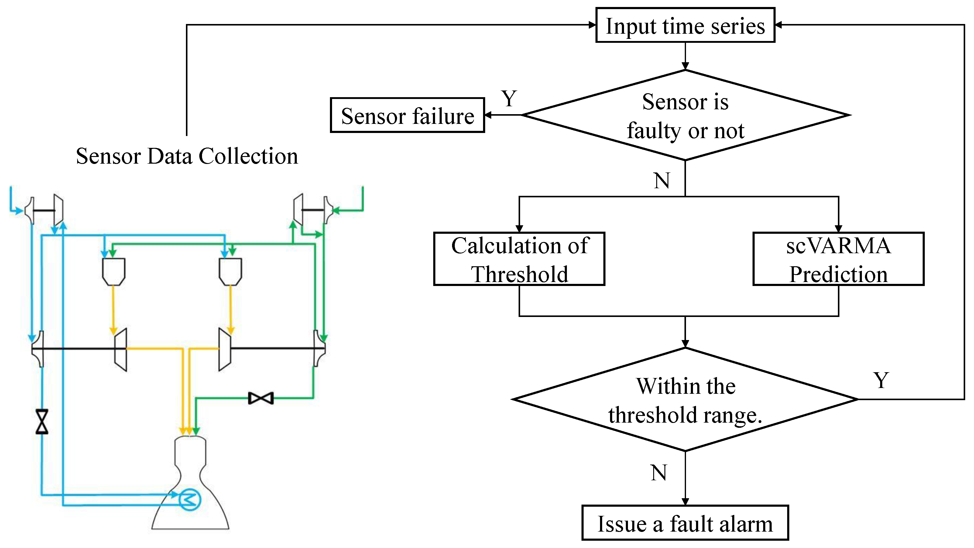
Once the threshold strategy is determined, the scVARMA is employed to predict parameters, thereby enabling fault prognosis. The comprehensive process is depicted in Figure 3. Data are first collected from sensors in the engine. Upon retrieval, an initial check is performed to determine the operational status of each sensor. If a sensor is found to be faulty, its data are discarded. For sensors operating normally, their data are used for predictive analysis. The scVARMA model predicts future parameter performance based on this data. Simultaneously, thresholds are calculated to determine if the predicted values fall within acceptable ranges. If a predicted value lies outside these thresholds, an alarm is triggered indicating a potential fault. Otherwise, the sensor parameters are considered normal, and monitoring continues. During the real-time input of time series data, the threshold is computed, and the established scVARMA model is utilized to predict future parameter performance. If the predicted values exceed the threshold range, a fault alarm is issued.

While establishing the model, typical historical data from engines of the same model are selected, and pre-processing is performed to stabilize the data, thereby fulfilling the application conditions for the scVARMA. For an established scVARMA, the predictive formula is expressed as follows:

$$\left[\begin{array}{c}{\widehat{y}}_n^T\\ {\widehat{y}}_{n-1}^T\\ ⋮\\ {\widehat{y}}_1^T\end{array}\right]=\left[\begin{array}{cccccc}{y}_{n-1}^T& \cdots & y_{n-p}^T& {\widehat{\epsilon }}_{n-1}^T& \cdots & {\widehat{\epsilon }}_{n-q}^T\\ y_{n-2}^T& \cdots & y_{n-1-p}^T& {\widehat{\epsilon }}_{n-2}^T& \cdots & {\widehat{\epsilon }}_{n-1-q}^T\\ ⋮& ⋮& ⋮& ⋮& ⋮& ⋮\\ y_0^T& \cdots & y_{1-p}^T& {\widehat{\epsilon }}_0^T& \cdots & {\widehat{\epsilon }}_{1-q}^T\end{array}\right]\times \left[\begin{array}{c}{\Phi }^T\\ {\Theta }^T\end{array}\right]$$

(11)

4. Experimental Validation

To evaluate the effectiveness of the scVARMA model in a real-world application, we conducted a two-fold experimental study. The first part of the study focused on online monitoring trials using a proprietary dataset from LRE, while the second part tested the predictive capabilities on both the proprietary dataset and a public dataset from the Case Western Reserve University Bearing Dataset.

4.1. Online Monitoring with Proprietary Data

The online monitoring experiment utilized real-time sensor data from the LRE to detect anomalies and predict potential failures. The dataset was derived from the results of a specific test run on an LRE. The sampling frequency of the sensors was uniformly 100 Hz. This research selected eleven parameters for analysis, each accompanied by its respective unit to ensure clarity and precision in data interpretation:

• Turbopump rotational speed (nt), unit: R/min;
• Kerosene primary pump discharge pressure (Pepf1), unit: MPa;
• Kerosene primary pump inlet pressure (Pipf1), unit: MPa;
• Oxygen pump discharge pulsation pressure (Pepo), unit: MPa;
• Oxygen pump inlet pressure (Pipo), unit: MPa;
• Pre-injector fuel pressure in the generator (Pihfg), unit: MPa;
• Pre-injector oxidizer pressure in the generator (Pohfg), unit: MPa;
• Flow regulator chamber pressure (Pitj), unit: MPa;
• Fuel throttle valve outlet pressure (PevjL), unit: MPa;
• Secondary and tertiary cooling band collector pressure (Pcj23), unit: MPa;
• Turbopump inlet temperature (Tit), unit: K.

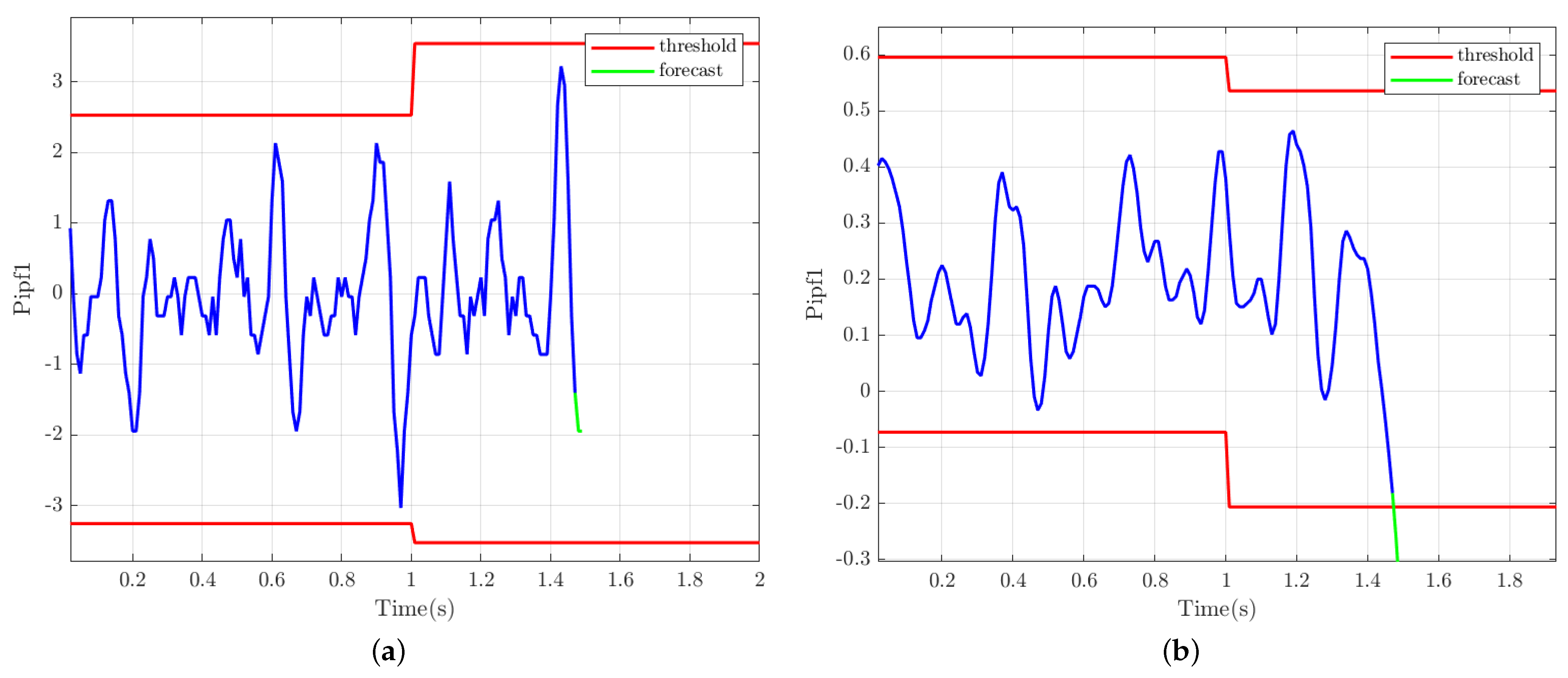
All data were subjected to first-order differencing and normalization processing to ensure data stationarity, thus meeting the data requirements for constructing the models. This experiment selected a segment of typical stable continuous data with 200 sample points for model construction. Here, we chose for p and q to be 11, respectively, for the scVARMA. The established coefficient lag matrix is illustrated in Figure 4. From the figure, it can be observed that many of the lag coefficients for pairs of parameters are zero, which greatly reduces the computational burden on the computer. When using scVARMA for one-step-ahead predictive online monitoring, taking the kerosene primary pump discharge pressure as an example, the results are illustrated in Figure 5, with the results under normal conditions on the right and the results under abnormal conditions on the left.

4.2. Predictive Performance on Proprietary and Public Data

The second part of the experiment evaluated the predictive performance of the scVARMA model. The experimental validation involved a detailed comparison with traditional ARMA and VARMA models across various sensors for predicting different system parameters.

Table 1. Mean and standard deviation of model in-sample fitting residuals.

Parameter	ARMA	ARMA_std	scVARMA_mean	scVARMA_std
nt	−0.0183	0.7018	−$2.1164\times {10}^{-11}$	0.7342
Pihfg	0.0126	0.6325	$3.1746\times {10}^{-11}$	0.5711
Pihog	−0.0042	0.5715	$1.5873\times {10}^{-11}$	0.5832
Pipf1	$1.1000\times {10}^{-10}$	1	$5.2910\times {10}^{-11}$	0.4193
Pepf1	0.0111	0.4966	−$1.0582\times {10}^{-11}$	0.4271
Pepo	−0.0166	0.6513	−$1.5273\times {10}^{-17}$	0.5856
Pipo	−0.0122	0.3755	$1.5873\times {10}^{-11}$	0.3936
PevjL	−0.0221	0.3569	−$1.5873\times {10}^{-11}$	0.3971
Pcj23	−0.0056	0.6032	$3.7037\times {10}^{-11}$	0.5809
Ptj	0.0079	0.4466	$1.0582\times {10}^{-11}$	0.4119
Tit	−0.0185	0.4297	−$5.2910\times {10}^{-12}$	0.4694

presents the mean and standard deviation of the residuals from the in-sample data fitting. The scVARMA model exhibits mean residuals close to zero and consistently lower standard deviations across most sensors, indicating better fitting to the in-sample data compared to both the ARMA and VARMA models. To further compare the predictive power,

Table 2. MAE and RMSE comparisons between ARMA, VARMA, and scVARMA models.

Sensor			Steps = 3						Steps = 5
	ARMA		VARMA		scVARMA		ARMA		VARMA		scVARMA
	MAE	RMSE	MAE	RMSE	MAE	RMSE	MAE	RMSE	MAE	RMSE	MAE	RMSE
nt	1.2488	0.4006	1.7797	0.4801	1.3117	0.4207	1.2190	0.4476	1.8639	0.4954	1.2599	0.4707
Pihfg	1.7167	0.7380	1.6594	0.7033	1.2203	0.6875	1.4510	0.6782	2.6932	0.6925	1.1725	0.6565
Pihog	1.6776	0.2555	1.1833	0.2152	0.2926	0.1925	2.1530	0.6805	2.4862	0.3841	0.4381	0.2042
Pipf1	0.5872	0.2646	0.7227	0.3259	1.3699	0.3648	0.4476	0.2717	1.2957	0.3601	1.0004	0.3863
Pepf1	1.4346	0.6650	1.3982	0.5017	0.7554	0.5147	1.7040	0.6010	1.9584	0.5233	0.9110	0.5018
Pepo	1.4330	0.8168	0.8688	0.8507	0.9232	0.7954	1.9060	0.9798	1.0446	0.8707	1.4425	0.9001
Pipo	0.8184	0.3496	0.3970	0.3304	0.2484	0.3167	0.6887	0.4531	0.4021	0.3197	0.3160	0.3913
PevjL	0.3277	0.1681	0.1878	0.2277	0.5236	0.2563	0.4234	0.3064	0.2212	0.3634	0.6109	0.3267
Pcj23	1.2339	0.9378	1.1325	0.9110	0.9680	0.8702	1.5379	0.8542	1.1468	0.8411	0.9882	0.8468
Ptj	1.6394	1.0069	1.1053	0.8013	1.1790	0.8337	1.9350	0.8513	1.1697	0.8120	1.3576	0.7966
Tit	0.1045	0.0748	0.7950	0.3281	0.7983	0.2601	0.1606	0.1267	0.8001	0.2917	0.8516	0.3145
mean	1.1111	0.5162	1.0209	0.5159	0.8719	0.5011	1.2387	0.5682	1.3711	0.5413	0.9408	0.5269

presents the mean absolute error (MAE) and root-mean-square error (RMSE) for both models at 3-step and 5-step predictions, highlighting the predictive accuracy across different future intervals. As shown in

Table 3. MAE and RMSE comparisons using the CWRU Bearing dataset.

Data	ARMA		VARMA		scVARMA
	MAE	RMSE	MAE	RMSE	MAE	RMSE
normal_0	0.1775	0.1230	0.1352	0.1218	0.1132	0.1164
normal_1	0.0086	0.0064	0.0081	0.0051	0.0063	0.0035
normal_2	0.0406	0.0241	0.0457	0.0356	0.0494	0.0299
normal_3	0.0485	0.0361	0.0493	0.0371	0.0323	0.0293

, the MAE and RMSE metrics of the scVARMA model have smaller values than the ARMA and VARMA models for most of the sensor data at 3 and 5 steps ahead of prediction.

To substantiate the universality of the proposed scVARMA model, we extended our evaluation to include the well-regarded Case Western Reserve University Bearing dataset. This dataset is a benchmark in the field of condition monitoring and predictive maintenance, consisting of vibration signal data that capture bearing performance under various conditions. For this phase of testing, this research specifically focused on the dataset’s normal operation conditions to align with the baseline comparisons established in earlier experiments. This analysis applied the ARMA, VARMA, and scVARMA models to predict the future states of the bearings and used the MAE and RMSE as metrics to assess the accuracy of these predictions. The outcomes are shown in Table 3.

5. Discussion

The results of our experiments on both proprietary and public datasets present a compelling case for the scVARMA model’s applicability in predictive maintenance and real-time monitoring. The improved prediction accuracy on both datasets when using the scVARMA model compared to the ARMA and VARMA models underscores the importance of considering cross-channel interactions.

In the experimental results, the scVARMA model shows the smallest increase in error as the prediction step increases from 3 to 5. This suggests that the scVARMA model is not only more accurate but also more stable over longer prediction horizons, likely due to its ability to effectively capture and utilize the interdependencies among multiple time series data. Additionally, by comparing the results of VARMA and scVARMA, although this study performs a sparse operation in identifying the parameters of the VARMA model, this rather leads to an increase in the predictive power. This may be due to the fact that the original VARMA model introduces redundant information when establishing relationships between different sequences. Performing a sparse operation can reduce the introduction of redundant information to some extent, which can improve the performance of the model to some extent.

6. Conclusions

In current engineering practices, ARMA models are predominantly used for online monitoring due to their simple structures, which meet the requirements for real-time processing. However, these models typically consider each channel independently, neglecting the interdependencies among various channels, which can be critical in complex system monitoring. Acknowledging this limitation, this study turned to the use of VARMA models, which are capable of capturing the dynamic interactions between multiple time series. Nevertheless, the extensive number of parameters in VARMA models poses a significant challenge for real-time forecasting due to their computational burden.

To mitigate this issue and pave the way for future real-time monitoring applications, the research introduced a sparsity-constrained approach to the VARMA structure. By enforcing sparsity, this method aimed to reduce model complexity without compromising the ability to model inter-channel dependencies. This adaptation of VARMA models not only makes real-time computation more feasible but also retains the essential characteristics needed for accurate monitoring and prediction in engineering systems.

The scVARMA model demonstrates promising results, offering a more sophisticated yet computationally efficient alternative to traditional ARMA models. It represents a step forward in the real-time health monitoring of complex systems, providing a foundation upon which future monitoring strategies can be developed to harness the full potential of multivariate time series analysis.

References

- Wang, C.; Zhang, Y.; Zhao, Z.; Chen, X.; Hu, J. Dynamic model-assisted transferable network for liquid rocket engine fault diagnosis using limited fault samples. Reliab. Eng. Syst. Saf. 2024, 243, 109837. [Google Scholar] [CrossRef]
- Biggs, R.E. Engineering the Engine: The Space Shuttle Main Engine. In Space Shuttle Legacy: How We Did It and What We Learned; Chapter 4; Launius, R.D., Krige, J., Craig, J.I., Eds.; American Institute of Aeronautics and Astronautics, Inc.: Reston, VA, USA, 2012; pp. 77–110. [Google Scholar]
- Williams, R.B., Jr.; Parlos, A.G. Adaptive state filtering for space shuttle main engine turbine health monitoring. J. Spacecr. Rocket. 2003, 40, 101–109. [Google Scholar] [CrossRef]
- Castenholz, P. Rocketdyne’s space shuttle main engine. In Proceedings of the 7th Propulsion Joint Specialist Conference, Salt Lake City, UT, USA, 14–18 June 1971; American Institute of Aeronautics and Astronautics, Inc.: Reston, VA, USA; p. 659. [Google Scholar]
- Oreilly, D. System for Anomaly and Failure Detection (SAFD) System Development (Final Report); Rockwell International Corp.: Canoga Park, CA, USA, 1993. [Google Scholar]
- Pérez-Roca, S.; Marzat, J.; Piet-Lahanier, H.; Langlois, N.; Farago, F.; Galeotta, M.; Le Gonidec, S. A survey of automatic control methods for liquid-propellant rocket engines. Prog. Aerosp. Sci. 2019, 107, 63–84. [Google Scholar] [CrossRef]
- Ma, M.; Zhong, Z.; Zhai, Z.; Sun, R. A novel optimal sensor placement method for optimizing the diagnosability of liquid rocket engine. Aerospace 2024, 11, 239. [Google Scholar] [CrossRef]
- Zhang, X.; Hua, X.; Zhu, J.; Ma, M. Intelligent Fault Diagnosis of Liquid Rocket Engine via Interpretable LSTM with Multisensory Data. Sensors 2023, 23, 5636. [Google Scholar] [CrossRef]
- Kashpruk, N.; Piskor-Ignatowicz, C.; Baranowski, J. Time Series Prediction in Industry 4.0: A Comprehensive Review and Prospects for Future Advancements. Appl. Sci. 2023, 13, 12374. [Google Scholar] [CrossRef]
- Zeng, A.; Chen, M.; Zhang, L.; Xu, Q. Are transformers effective for time series forecasting? In Proceedings of the AAAI Conference on Artificial Intelligence, Washington, DC, USA, 7–14 February 2023; Volume 37, pp. 11121–11128. [Google Scholar] [CrossRef]
- Dissanayake, P.; Flock, T.; Meier, J.; Sibbertsen, P. Modelling short-and long-term dependencies of clustered high-threshold exceedances in significant wave heights. Mathematics 2021, 9, 2817. [Google Scholar] [CrossRef]
- Irshad, M.R.; Aswathy, S.; Maya, R.; Nadarajah, S. New One-Parameter Over-Dispersed Discrete Distribution and Its Application to the Nonnegative Integer-Valued Autoregressive Model of Order One. Mathematics 2023, 12, 81. [Google Scholar] [CrossRef]
- Liu, Y.; Garg, S.; Nie, J.; Zhang, Y.; Xiong, Z.; Kang, J.; Hossain, M.S. Deep anomaly detection for time-series data in industrial IoT: A communication-efficient on-device federated learning approach. IEEE Internet Things J. 2020, 8, 6348–6358. [Google Scholar] [CrossRef]
- Kim, B.; Alawami, M.A.; Kim, E.; Oh, S.; Park, J.; Kim, H. A comparative study of time series anomaly detection models for industrial control systems. Sensors 2023, 23, 1310. [Google Scholar] [CrossRef] [PubMed]
- Mandrikova, O.; Mandrikova, B.; Esikov, O. Detection of Anomalies in Natural Complicated Data Structures Based on a Hybrid Approach. Mathematics 2023, 11, 2464. [Google Scholar] [CrossRef]
- Ma, M.; Fu, L.; Zhai, Z.; Sun, R.B. Transformer based Kalman Filter with EM algorithm for time series prediction and anomaly detection of complex systems. Measurement 2024, 229, 114378. [Google Scholar] [CrossRef]
- Momin, B.; Chavan, G. Univariate time series models for forecasting stationary and non-stationary data: A brief review. In Information and Communication Technology for Intelligent Systems (ICTIS 2017)-Volume 2; Springer: Cham, Switzerland, 2018; pp. 219–226. [Google Scholar]
- Fiorucci, T.; Lakin, D., II; Reynolds,, T. Advanced engine health management applications of the SSME real-time vibration monitoring system. In Proceedings of the 36th AIAA/ASME/SAE/ASEE Joint Propulsion Conference and Exhibit, Las Vegas, NV, USA, 14–28 July 2000; p. 3622. [Google Scholar]
- Deng, C.; Xue, W.; Zheng, M.; Ma, H. Study on Real Time Diagnosis Method of the Main Stage Working Condition of Rocket Engine Based on Improved ARMA Model. Comput. Meas. Control 2020, 28, 33–38. [Google Scholar]
- Zhao, W.; Guo, Y.; Yang, J.; Sun, H. Hardware-in-the-loop simulation platform for fault diagnosis of rocket engines. In Proceedings of the 2019 IEEE 10th International Conference on Mechanical and Aerospace Engineering (ICMAE), Brussels, Belgium, 22–25 July 2019; IEEE: New York, NY, USA, 2019; pp. 268–273. [Google Scholar]
- Xue, W.; Zhang, Q.; Wu, X. Based on the ARMA Model for the Liquid Rocket Propulsion Fault Detection. Comput. Meas. Control 2019, 27, 4–7. [Google Scholar]
- Deng, L.; Cheng, Y.; Shi, Y. Fault detection and diagnosis for liquid rocket engines based on long short-term memory and generative adversarial networks. Aerospace 2022, 9, 399. [Google Scholar] [CrossRef]
- Nicholson, W.B.; Matteson, D.S.; Bien, J. VARX-L: Structured regularization for large vector autoregressions with exogenous variables. Int. J. Forecast. 2017, 33, 627–651. [Google Scholar] [CrossRef]
- Davis, R.A.; Zang, P.; Zheng, T. Sparse vector autoregressive modeling. J. Comput. Graph. Stat. 2016, 25, 1077–1096. [Google Scholar] [CrossRef]
- Runkle, D.E. Vector autoregressions and reality. J. Bus. Econ. Stat. 1987, 5, 437–442. [Google Scholar] [CrossRef]
- Box, G.E.; Jenkins, G.M.; Reinsel, G.C.; Ljung, G.M. Time Series Analysis: Forecasting and Control; John Wiley & Sons: Hoboken, NJ, USA, 2015. [Google Scholar]
- Lütkepohl, H. New Introduction to Multiple Time Series Analysis; Springer Science & Business Media: Berlin/Heidelberg, Germany, 2005. [Google Scholar]
- Brockwell, P.J.; Davis, R.A. Time Series: Theory and Methods; Springer Science & Business Media: Berlin/Heidelberg, Germany, 1991. [Google Scholar]
- Hannan, E.J.; Kavalieris, L. Multivariate linear time series models. Adv. Appl. Probab. 1984, 16, 492–561. [Google Scholar] [CrossRef]
- Tibshirani, R. Regression shrinkage and selection via the lasso. J. R. Stat. Soc. Ser. B Stat. Methodol. 1996, 58, 267–288. [Google Scholar] [CrossRef]
- Koop, G.; Korobilis, D. Bayesian multivariate time series methods for empirical macroeconomics. Found. Trends® Econom. 2010, 3, 267–358. [Google Scholar] [CrossRef]
- Nicholson, W.B.; Matteson, D.S.; Bien, J. Structured Regularization for Large Vector Autoregression. Ph.D. Thesis, Cornell University, Ithaca, NY, USA, 2014. [Google Scholar]
- Spliid, H. A fast estimation method for the vector autoregressive moving average model with exogenous variables. J. Am. Stat. Assoc. 1983, 78, 843–849. [Google Scholar] [CrossRef]
- Dufour, J.M.; Jouini, T. Asymptotic distributions for quasi-efficient estimators in echelon VARMA models. Comput. Stat. Data Anal. 2014, 73, 69–86. [Google Scholar] [CrossRef]
- Dolgopolov, S.I.; Nikolayev, O.D.; Khoriak, N.V. Dynamic interaction between clustered liquid propellant rocket engines under their asynchronous start-ups. Propuls. Power Res. 2021, 10, 347–359. [Google Scholar] [CrossRef]
- Park, S.Y.; Ahn, J. Deep neural network approach for fault detection and diagnosis during startup transient of liquid-propellant rocket engine. Acta Astronaut. 2020, 177, 714–730. [Google Scholar] [CrossRef]
- Pérez-Roca, S.; Marzat, J.; Piet-Lahanier, H.; Langlois, N.; Galeotta, M.; Farago, F.; Le Gonidec, S. Model-based robust transient control of reusable liquid-propellant rocket engines. IEEE Trans. Aerosp. Electron. Syst. 2020, 57, 129–144. [Google Scholar] [CrossRef]
- Cha, J.; Ko, S.; Park, S.Y.; Jeong, E. Fault detection and diagnosis algorithms for transient state of an open-cycle liquid rocket engine using nonlinear Kalman filter methods. Acta Astronaut. 2019, 163, 147–156. [Google Scholar] [CrossRef]
- Durrett, R. Probability: Theory and Examples; Cambridge University Press: Cambridge, UK, 2019; Volume 49. [Google Scholar]
Figure 1.
System diagram of LRE [22]. (1. Fuel pre-pressurization turbopump; 2. oxidizer pre-pressurization turbopump; 3. gas generator; 4. main turbine; 5. oxidizer pump; 6. fuel primary pump; 7. fuel secondary pump; 8. thrust chamber; 9. throttle valve; 10. flow regulator; 11. starter box; 12. ignition duct).
Figure 2.
Schematic Diagram of System Failure Progression.
Figure 3.
Online monitoring process.
Figure 4.
(a) AR-lag matrix and (b) MA-lag matrix of the estimated VARMA.
Figure 5.
One-step Predictive Online monitoring results for rotational speed: (a) Normal data and (b) Failure data.