A Reentry Trajectory Planning Algorithm via Pseudo-Spectral Convexification and Method of Multipliers

Abstract

The reentry trajectory planning problem of hypersonic vehicles is generally a continuous and nonconvex optimization problem, and it constitutes a critical challenge within the field of aerospace engineering. In this paper, an improved sequential convexification algorithm is proposed to solve it and achieve online trajectory planning. In the proposed algorithm, the Chebyshev pseudo-spectral method with high-accuracy approximation performance is first employed to discretize the continuous dynamic equations. Subsequently, based on the multipliers and linearization methods, the original nonconvex trajectory planning problem is transformed into a series of relaxed convex subproblems in the form of an augmented Lagrange function. Then, the interior point method is utilized to iteratively solve the relaxed convex subproblem until the expected convergence precision is achieved. The convex-optimization-based and multipliers methods guarantee the promotion of fast convergence precision, making it suitable for online trajectory planning applications. Finally, numerical simulations are conducted to verify the performance of the proposed algorithm. The simulation results show that the algorithm possesses better convergence performance, and the solution time can reach the level of seconds, which is more than 97% less than nonlinear programming algorithms, such as the sequential quadratic programming algorithm.

1. Introduction

Hypersonic vehicles generally refer to near-space vehicles with flight speeds greater than Mach 5. They possess the advantages of strong maneuverability, flexible trajectory, they are difficult to intercept, and so on, and they have been increasingly valued by the major space powers due to their high flight speeds and vast airspace coverage. Among the related technologies, trajectory planning technology can provide important support for performance analysis regarding flight range, maneuverability, and ballistic characteristics. The hypersonic vehicle trajectory planning problem typically involves solving a nonlinear optimal control problem with various state and control constraints, including boundary conditions, no-fly-zone constraints, path constraints, etc. [1,2,3].

In this regard, many scholars and engineers have carried out a series of in-depth studies, and the proposed trajectory planning algorithms generally include indirect and direct methods. The indirect methods transform the trajectory planning problem into a Hamiltonian boundary value problem based on the Pontryagin maximum principle and solves it by employing the gradient method and other algorithms. On the other hand, many scholars have proposed and developed the collocation method, pseudo-spectral method, and other methods [4,5,6,7], demonstrating the advantages of direct methods in solving trajectory optimization problems. However, the direct methods still have some shortcomings under the requirement of rapid trajectory planning, such as high sensitivity to initial guess value and uncertain solving time and convergence, which restrict their efficient solving ability [8].

In recent years, convex-optimization-based methods have effectively met the demand for efficient solutions and attracted more and more attention in terms of spacecraft trajectory optimization. When a problem can be formulated within a convex optimization framework, its complexity is low and can be reliably solved to global optimality in the polynomial time by the primal-dual interior point method. The upper bound of the number of iterations required for convergence is also determined. Moreover, the primal-dual interior point method can be adopted to solve the convex problem without the initial guess value. Motivated by these preponderances, the convex-optimization-based methods have been applied to different aerospace problems, such as planetary reentry trajectory optimization [9], ascent trajectory optimization [10,11], Mars-landing trajectory planning [12,13], low-thrust orbit transfer [14], spacecraft rendezvous and proximity operations [15,16], and trajectory planning for satellite cluster reconfigurations [17].

Most aerospace problems are limited by nonlinear, nonconvex dynamics and path constraints, so they cannot be solved directly under the convex optimization framework. Therefore, convexification technologies that make the approximate error as small as possible are a significant research direction [18]. Among them, the two mainstream convexification methods include lossless convexification and sequential convexification methods. In Refs. [12,13], Ackimese et al. employed the lossless convexification method to solve the Mars-landing trajectory planning problem by replacing nonconvex constraints with relaxed convex constraints without a loss of accuracy. But the lossless convexification method is only suitable for a few constraints with particular forms, which limits its wide application. On the other hand, the sequential convexification method can conduct highly nonlinear complex problems. The basic idea is to obtain a series of convex subproblems by approximating the nonlinear terms and then solve them iteratively until it converges to the expected precision [19,20].

However, the sequential convexification method can be further improved in terms of discretization and accelerating convergence. Firstly, the traditional trapezoidal discrete method [3,19,20] is often chosen to discretize the continuous optimization problem, which leads to a large deviation between the approximate model used in the solution procedure and the actual one. To obtain a precise-enough solution, the equidistant discrete nodes should be sufficiently numerous. Nevertheless, it also results in a dramatic increase in the number of optimization variables and takes lots of time to solve. In contrast, the pseudo-spectral discretization methods offer higher accuracy under the same number of discrete nodes and have been widely employed for solving the optimal control problem [5,8]. Among the pseudo-spectral methods, the Chebyshev pseudo-spectral discretization method [21,22] is a special category, which can minimize the Runge phenomenon and supply the best polynomial approximation under the minimax norm. On the other hand, “artificial infeasibility” [23,24] caused by the convexification errors occurs when the original problem is feasible but the convex subproblem is not. Researchers address this issue by introducing slack variables to relax the feasible domain limited by various constraints, with large constant penalty parameters added to penalize these slack variables. As a result, the “artificial infeasible” gradually disappears and the slack variables tend towards zero as the iterative solution converges. Unfortunately, the fixed penalty parameters could cause the solution to converge to a stagnation point of the penalty problem rather than the original problem, according to Ref. [25].

To address the aforementioned issues, an improved sequential convexification algorithm is proposed to improve the performance of solving the trajectory planning problem of hypersonic vehicles in this paper. Firstly, the Chebyshev pseudo-spectral method with higher approximation precision is employed to discretize the continuous optimal control problem. And the flight terminal time is designed as an optimization variable, so that it can be applied to the optimal control problem with a fixed initial state and free terminal state. Then, by introducing automatically updated penalty parameters and Lagrange multipliers, the relaxed convex subproblem in the form of the augmented Lagrange function is constructed to improve the convergence and computational properties based on the method of multipliers (or the augmented Lagrange method). And it is solved iteratively by the interior point method in the framework of the improved sequential convexification algorithm.

The rest of this paper is organized as follows. In Section 2, the reentry trajectory optimization problem is formulated. In Section 3, the improved sequential convexification algorithm is detailed. In Section 4, numerical simulations are presented to verify the performance of the algorithm. Finally, the conclusion and discussion are provided in Section 5.

2. Problem Formulation

2.1. Reentry Dynamics

In view of the dynamics characteristics of the reentry flight of hypersonic vehicles, the dimensionless three-degrees-of-freedom augmented dynamics model is established in the half-velocity coordinate system without considering Earth’s flatness and rotation:

$$\{\begin{array}{l}\dot{r}=v\sin \gamma \\ \dot{\theta }=v\cos \gamma \sin \psi /(r\cos \varphi )\\ \dot{\varphi }=v\cos \gamma \cos \psi /r\\ \dot{v}=-D-\sin \gamma /r^2\\ \dot{\gamma }=L\cos \sigma /v+(v^2-1/r)\cos \gamma /(vr)\\ \dot{\psi }=L\sin \sigma /(v\cos \gamma )+v\cos \gamma \sin \psi \tan \varphi /r\\ \dot{\sigma }=u\end{array},$$

(1)

where $r$ is the radial distance from the Earth center to the vehicle, $\theta$ and $\varphi$ are the longitude and latitude, respectively, $v$ is the velocity, $\gamma$ is the flight path angle, $\psi$ is the heading angle, and $\sigma$ is the bank angle. The above variables are defined as system state variables, i.e., $x={[r,v,\theta ,\varphi ,\gamma ,\psi ,\sigma ]}^T$, and the control variable is the bank angle rate $u\in R$. The variables $r$, $v$ and time are scaled by $R_0$, $\sqrt{R_0{g}_0}$ and $\sqrt{R_0/g_0}$, respectively, where $R_0=6371\mathrm{km}$ is the Earth radius and $g_0=9.8 {\mathrm{m}/\mathrm{s}}^2$ is the gravitational acceleration at sea level. Dimensionless lift and drag accelerations $L$ and $D$ are scaled by $g_0$ and calculated as:

$$\begin{array}{l}L=\frac{R_0\rho v^{2}S{C}_L}{2m}\\ D=\frac{R_0\rho v^{2}S{C}_D}{2m}\end{array},$$

(2)

where $m$ is the vehicle mass, $S$ is the reference area of the vehicle, and $\rho$ is the atmospheric density, $\rho ={\rho }_0{e}^{-H/H_s}$, where $H=r{R}_0-R_0$ is the height, $H_s$ is the atmospheric density scale height, and ${\rho }_0$ is the atmospheric density at sea level. Moreover, $C_L$ and $C_D$ are lift and drag coefficients, respectively. For reference to the aerodynamic parameters of the vehicle in [9], the aerodynamic coefficient can be expressed as:

$$\{\begin{array}{l}{C}_L=-0.041065+0.016292\alpha +0.0002602{\alpha }^2\\ C_D=0.080505-0.03026C_L+0.86495C_L^2\end{array},$$

(3)

in which the angle of attack $\alpha$ is in degree and expressed as a function of velocity. The angle-of-attack velocity profile is preset as follows:

$$\alpha =\{\begin{array}{l}40, v\sqrt{R_0{g}_0}>4570\mathrm{m}/\mathrm{s}\\ 40-0.20705\frac{{(v\sqrt{R_0{g}_0}-4570)}^2}{{340}^2}, \mathrm{otherwise}\end{array}.$$

(4)

In general, the design of the bank angle is the main means to change the trajectory of the vehicle when the angle of attack is preset. However, the bank angle rate is adopted here as the new control variable for the following reasons. Firstly, boundary constraints are applied to make the bank angle profile smoother. Secondly, the current system dynamics are transformed into affine control form, which expedite subsequent convexification operations and alleviate the high-frequency fluctuations in the bank angle [9].

2.2. Constraint Conditions

The trajectory planning problem of hypersonic vehicles belongs to a class of optimal control problems, and its purpose is to determine the optimal control variables and optimize the performance index function under various constraints.

Generally, the vehicle must meet different constraints, such as heat rate, dynamic pressure, load, and control margin, during the ultra-high-speed flight to ensure the safety of the vehicle structure, thermal protection, guidance, and control systems. To meet the mission requirements, the initial conditions and terminal states of the vehicle also need to be limited. In addition, the vehicle should avoid certain no-fly zones due to radar detection, geopolitics, or other considerations. In summary, all of these constraint conditions can be divided into two categories: equality constraints and inequality constraints.

First of all, the equality constraints mainly include dynamic equations and initial and terminal constraints. Here, the system dynamics Equation (1) is abstractly expressed as

$$\dot{x}=f(x,u,t)=f_0(x,t)+Bu,$$

(5)

where $t$ is the system time variable, and $f(·,·,·)$ is the right function of the dynamic equations. And $f_0(x,t)=\{\begin{array}{l}v\sin \gamma \\ v\cos \gamma \sin \psi /(r\cos \varphi )\\ v\cos \gamma \cos \psi /r\\ -D-\sin \gamma /r^2\\ L\cos \sigma /v+(v^2-1/r)\cos \gamma /(vr)\\ L\sin \sigma /(v\cos \gamma )+v\cos \gamma \sin \psi \tan \varphi /r\\ 0\end{array}$, $B={[0,0,0,0,0,0,1]}^T$.

The initial and terminal constraints are determined by the flight mission, which contains the requirements of the reentry start point and the target point, and they can be represented as follows:

$$\begin{array}{l}\Phi (x(t_0),x_0)=0\\ \Psi (x(t_f),x_f)=0\end{array},$$

(6)

where $t_0$ and $t_f$ are the initial and terminal time, respectively. $\Phi (·,·)$ and $\Psi (·,·)$ are the initial and terminal state constraints, respectively.

Then, inequality constraints can be divided into the following three categories. First, the path constraints, including the maximal heat rate, dynamic pressure, and load, are expressed as:

$$p(r,v)=\left[\begin{array}{l}\dot{Q}-{\dot{Q}}_{\max }\\ q-q_{\max }\\ n-n_{\max }\end{array}\right]=\left[\begin{array}{l}{K}_Q{\rho }^{0.5}{(v\sqrt{R_0{g}_0})}^{3.15}-{\dot{Q}}_{\max }\\ 0.5\rho {(v\sqrt{R_0{g}_0})}^2-q_{\max }\\ \sqrt{L^2+D^2}-n_{\max }\end{array}\right]\le 0,$$

(7)

where ${\dot{Q}}_{\max }$, $q_{\max }$ and $n_{\max }$ are the corresponding maximum values, respectively.

Second, the bounded constraints about the state and control variables are given by:

$$\begin{array}{l}{x}_{\min }\le x\le x_{\max }\\ u_{\min }\le u\le u_{\max }\end{array},$$

(8)

where ${·}_{\min }$ and ${·}_{\max }$ are the lower and upper bound values, respectively.

The last class of inequality constraints is the no-fly-zone (NFZ) constraint. In general, an NFZ is modeled as a circular exclusion zone in the horizontal place with infinite height and limits the longitude and latitude of the flight trajectory by

$${(\theta -{\theta }_c)}^2+{(\varphi -{\varphi }_c)}^2\ge d^2,$$

(9)

where ${\theta }_c$ and ${\varphi }_c$ are the longitude and latitude at the center of the NFZ, and $d$ is the radius.

2.3. Optimal Control Problem

In the trajectory optimization problem, the performance indexes can be reasonably selected according to the different flight tasks and design requirements. Common performance indexes include minimum flight time, maximum range, minimum heat load, etc. In this paper, the minimum flight time is chosen as the performance index, considering that the vehicle needs to reach the anticipative target point quickly. Henceforth, the original reentry trajectory optimization problem can be formulated as a highly constrained optimal control problem:

$$\begin{array}{l}{P}_0: min J={\displaystyle {\int }_0^{t_f}1 dt}\\ s.t. Eq. (5),(6),(7),(8),(9)\end{array}.$$

3. Improved Sequential Convexification Algorithm

In this section, an augmented Lagrange-based Chebyshev pseudo-spectral form improved sequential convexification (AL-CP-ISC) algorithm is proposed to solve the above continuous and nonlinear reentry trajectory optimization problem. The advantages of the pseudo-spectral method with high discrete accuracy and the method of multipliers with good convergence performance and stable numerical computation are synthesized to empower the AL-CP-ISC algorithm. Firstly, the discretization and convexification process of the vehicle’s nonlinear system are given on the strength of the Chebyshev pseudo-spectral method and first-order Taylor expansion. Subsequently, the original problem is transformed into a series of relaxed convex subproblems by introducing the slack variables, penalty parameters, and Lagrange multipliers. Finally, an algorithm solution procedure is presented.

3.1. Discretization and Convexification

The Chebyshev pseudo-spectral discretization method with unique time-domain mapping is adopted to discretize the continuous reentry trajectory optimization problem $P_0$ with the free terminal time. In the Chebyshev pseudo-spectral discretization method, the domain of the Chebyshev–Gauss–Lobatto (CGL) points is $\tau \in [-1,1]$, but the flight time interval is $t\in [t_0,t_f]$ in the practical problem. Hence, the time variable is transformed into

$$\tau =\frac{2t}{t_f-t_0}-\frac{t_f+t_0}{t_f-t_0}.$$

(10)

The CGL points are unevenly distributed on the interval $[-1,1]$:

$${\tau }_k=\cos \left(\frac{\pi k}{N}\right) k=0,\dots ,N.$$

(11)

Taking the real state and control variables at $N+1$ nodes above, the Lagrange interpolation polynomials are constructed, respectively, as approximations of continuous state and control variables. The approximate expressions of the real state variable $x$ and the control variable $u$ are

$$\begin{array}{l}x\left(\tau \right)\approx x^N\left(\tau \right)={\displaystyle \sum _{j=0}^N{x}_j{\varphi }_j\left(\tau \right)}\\ u\left(\tau \right)\approx u^N\left(\tau \right)={\displaystyle \sum _{j=0}^N{u}_j{\varphi }_j\left(\tau \right)}\end{array},$$

(12)

where ${\varphi }_j(\tau )$ is the $N^{th}$ Lagrange interpolation basis function

$${\varphi }_j\left(\tau \right)=\frac{{\left(-1\right)}^{j+1}}{N^2{c}_j}\frac{\left(1-{\tau }^2\right){\dot{T}}_N\left(\tau \right)}{\tau -{\tau }_j},$$

(13)

where $T_N(\tau )$ is the $N\mathrm{th}-\mathrm{order}$ Chebyshev polynomial and

$$c_j=\{\begin{array}{l}2,j=0,N\\ 1,1\le j\le N-1\end{array}.$$

(14)

Deriving the approximate expression for the state variables $x(\tau )$ yields:

$$\dot{x}\left({\tau }_k\right)\approx {\dot{x}}^N\left({\tau }_k\right)={\displaystyle \sum _{j=0}^N{x}_j{\dot{\varphi }}_j\left({\tau }_k\right)}={\displaystyle \sum _{j=0}^N{D}_{kj}{x}_j}$$

(15)

where $D_{kj}$ is the $k^{th}$ row and $j^{th}$ column element of the differential matrix $D^{(N+1)\times (N+1)}$ of the Chebyshev pseudo-spectral discretization method, and the calculation of each element’s value of the matrix $D$ is shown in Ref. [21].

The derivatives of the state variables in the dynamic equations are replaced using the right-hand term in Equation (15) and discretized at the nodes, so that the original differential dynamic equation constraints are transformed into discrete algebraic constraints:

$$2{\displaystyle \sum _{j=0}^N{D}_{kj}{x}_j+(t_0-t_f^k)}f(x_k,u_k,t_k)=2{\displaystyle \sum _{j=0}^N{D}_{kj}{x}_j+(t_0-t_f^k)}{f}_0(x_k,t_k)+(t_0-t_f^k)B{u}_k=0 k=0,1,\cdots ,N.$$

(16)

Next, the above nonlinear algebraic constraints are linearized based on first-order Taylor expansion as follows:

$$2{\displaystyle \sum _{j=0}^N{D}_{kj}}{x}_j+A(x^{*},{t_f}^{*})x+(t_0-{t_f}^{*})Bu+[T(x^{*},{t_f}^{*})-B{u}^{*}]t_f+C=0,$$

(17)

where $x^{*},u^{*}$ and $t_f^{*}$ are the reference values of the optimization variables $[x,u,t_f]$, respectively, and

$$A(x^{*},{t_f}^{*})=\frac{\partial [(t_0-t_f)f_0(x,t)]}{\partial x}{|}_{x=x^{*},t_f={t_f}^{*}}=(t_0-{t_f}^{*})\frac{\partial f_0(x,t)}{\partial x}{|}_{x=x^{*}},$$

(18)

$$(t_0-{t_f}^{*})B={[0,0,0,0,0,0,(t_0-{t_f}^{*})]}^T,$$

(19)

$$T(x^{*},{t_f}^{*})=\frac{\partial [(t_0-t_f)f_0(x,t)]}{\partial t_f}{|}_{x=x^{*},t_f={t_f}^{*}}=-f_0(x,t){|}_{x=x^{*}},$$

(20)

$$C=(t_0-t_f^{*})f_0^{*}-A(x^{*},t_f^{*})x^{*}-T(x^{*},t_f^{*})t_f^{*}+B{u}^{*}{t}_f^{*}.$$

(21)

One can see Appendix A for more details on the matrix $A$. Similarly, the nonlinear path constraints are given by:

$$p(x)=\left[\begin{array}{l}\dot{Q}(x)-{\dot{Q}}_{\max }\\ q(x)-q_{\max }\\ n(x)-n_{\max }\end{array}\right]\approx \left[\begin{array}{l}\dot{Q}(x^{*})+\nabla \dot{Q}(x^{*})(x-x^{*})-{\dot{Q}}_{\max }\\ q(x^{*})+\nabla q(x^{*})(x-x^{*})-q_{\max }\\ n(x^{*})+\nabla n(x^{*})(x-x^{*})-n_{\max }\end{array}\right]\le 0,$$

(22)

where

$$\begin{array}{l}\nabla \dot{Q}(x^{*})=[\frac{\partial \dot{Q}}{\partial r},\frac{\partial \dot{Q}}{\partial v}]=[-0.5k_Q{(v\sqrt{R_0{g}_0})}^{3.15}\frac{\sqrt{\rho }}{H_s},3.15k_Q{(\sqrt{R_0{g}_0})}^{3.15}{v}^{2.15}\sqrt{\rho }]{|}_{x=x^{*}}\\ \nabla q(x^{*})=[\frac{\partial q}{\partial r},\frac{\partial q}{\partial v}]=[-0.5{(v\sqrt{R_0{g}_0})}^2\frac{R_0\rho }{H_s},{(\sqrt{R_0{g}_0})}^2\rho v]{|}_{x=x^{*}}\\ \nabla n(x^{*})=[\frac{\partial n}{\partial r},\frac{\partial n}{\partial v}]=[-0.5R_0^{2}S\sqrt{C_L^2+C_D^2}\frac{\rho v^2}{m{H}_s},R_{0}S\sqrt{C_L^2+C_D^2}\frac{\rho v}{m}]{|}_{x=x^{*}}\end{array}.$$

(23)

The NFZ constraint is a nonconvex function and also needs to be convexified by the first-order Taylor expansion, as shown below:

$$2({\theta }^{*}-{\theta }_c)\theta +2({\varphi }^{*}-{\varphi }_c)\varphi \ge d^2+\tilde{d},$$

(24)

where

$$\tilde{d}=-{({\theta }^{*}-{\theta }_c)}^2-{({\varphi }^{*}-{\varphi }_c)}^2+2({\theta }^{*}-{\theta }_c){\theta }^{*}+2({\varphi }^{*}-{\varphi }_c){\varphi }^{*}.$$

(25)

Finally, to place limits on the deviation of the state variables between the linearized and original system, a trust region constraint is introduced, so as to reduce the linearization error and improve the convergence of the sequential linear approximation, denoted as

$$\Vert x-x^{*}\Vert \le \delta ,$$

(26)

where $\delta \in {ℝ}^7$ is a constant vector, and the inequality is expressed in components. This is a second-order conic constraint that is, itself, convex. Adding the trust region constraint is necessary to guarantee the linearized constraints to legitimately approximate the original constraints. Meanwhile, proposition 2 in Ref. [9] theoretically explains that a feasible solution of the linearized problem satisfies the linearized path constraints, and it also satisfies the original path constraints.

Up to now, all the continuous and nonconvex functions in the trajectory optimization problem have been discretized and convexified, and the problem $P_0$ is converted into a discretized convex problem:

$$\begin{array}{l}DC{P}_0: min J={\displaystyle {\int }_0^{{\tau }_f}1 dt}\\ s.t. Eq. (6),(8),(17),(22),(24),(26)\end{array}.$$

3.2. Problem Transformation

Combining the discretization and convexification processes, the original problem is transformed into an augmented Lagrange formal convex problem. The AL-CP-ISC algorithm can profit from this conversion, resulting in convergence-rate promotion and numerical difficulty avoidance according to the following analysis [26,27,28].

The linearized error causes the feasible region of the original problem to shrink to a certain extent in the process of convexification, resulting in the “artificial infeasible” situation in which the original problem is feasible but the linearized problem is not feasible. Hereon, slack variables are introduced to relax the “hard constraints”, such as dynamic equations, path constraints, and terminal conditions, to compensate for the linearization errors [8,18]. In the meantime, penalty parameters are introduced to punish the slack variables. When the iterative solution converges, the slack variables also gradually approach zero due to the penalty imposed. However, the penalty parameters are usually selected as a larger constant value in many studies of spacecraft trajectory optimization. Unfortunately, the constant penalty parameters can cause the iterative solution to converge to the stationary point of the penalty problem instead of the original problem [25].

Therefore, to resolve this matter, the slack variables are penalized by penalty parameters, which are automatically updated incrementally. Meanwhile, to prevent the condition number of the Hessian matrix from getting worse and worse when the penalty parameters are updated to infinity, which leads to numerical difficulties in the algorithm, Lagrange multipliers are introduced to transform the penalty function problem into the augmented Lagrange function one. According to the augmented Lagrange function method, by embedding the multiplier update mechanism, the satisfaction degree of constraints and the optimization of the objective function can be considered in each iteration, thus reducing the number of iterations required to achieve the same precision. Additionally, the augmented Lagrange function method can also effectively control the condition number of the Hessian matrix through its unique construction, which avoids the instability of numerical computation. In short, the iterative solution of the algorithm can converge to the solution of the original problem, and the penalty parameters do not need to go to infinity.

Here, the original problem is abstracted into a general nonlinear programming problem form to illustrate the relaxed convex problem of an augmented Lagrange form, as shown below:

$$\begin{array}{l}{P}_1 \min J={\displaystyle {\int }_0^{{\tau }_f}1 dt}={\tau }_f\\ s.t. h_i(\widehat{x})=0,i\in {\rm E}\\ g_i(\widehat{x})\le 0,i\in {\rm I}\\ s_i(\widehat{x})\in K,i\in C\end{array},$$

where $\widehat{x}={[x,u,t_f]}^T$ are augmented optimization variables, all equality constraints are denoted as $h(\widehat{x})$, all inequality constraints are expressed as $g(\widehat{x})$, and $s(\widehat{x})$ represents the second-order cone constraints. And ${\rm E}$, ${\rm I}$, and $C$ are the corresponding feasible domain sets, respectively.

Then, the slack variables ${\zeta }_h,{\zeta }_g$, penalty parameters $p$, and Lagrange multipliers $\mu ,\lambda$ are introduced to construct the relaxed problem of augmented Lagrange function form as follows:

$$\begin{array}{l}{P}_2 \min \tilde{J}(\widehat{x},{\zeta }_h,{\zeta }_g)={\tau }_f+{\lambda }^T{\zeta }_h+p\left|{\zeta }_h\right|+{\mu }^T{\zeta }_g+p\left|{\zeta }_g\right|\\ s.t. h_i(\widehat{x})={\zeta }_{i,h},i\in {\rm E}\\ g_i(\widehat{x})\le {\zeta }_{i,g},{\zeta }_{i,g}\ge 0,i\in {\rm I}\\ s_i(\widehat{x})\in K,i\in C\end{array},$$

where, for further transformation, the penalty term of the inequality function is not treated as a standard cutoff function because the slack variables ${\zeta }_g$ are nonnegative but as an absolute value term. The similar treatment method can also be found in Ref. [25].

Finally, the problem $P_2$ is convexified by the first-order Taylor expansion:

$$\begin{array}{l}{P}_3 \min \tilde{J}(\Delta \widehat{x},{\zeta }_h^k,{\zeta }_g^k)={\tau }_f+{({\lambda }^k)}^T{\zeta }_h^k+p^k\left|{\zeta }_h^k\right|+{({\mu }^k)}^T{\zeta }_g^k+p^k\left|{\zeta }_g^k\right|\\ s.t. h_i({\widehat{x}}^k)+\nabla h_i({\widehat{x}}^k)\Delta \widehat{x}={\zeta }_{i,h}^k,i\in {\rm E}\\ g_i({\widehat{x}}^k)+\nabla g_i({\widehat{x}}^k)\Delta \widehat{x}\le {\zeta }_{i,g}^k,{\zeta }_{i,g}^k\ge 0,i\in {\rm I}\\ s_i({\widehat{x}}^k+\Delta \widehat{x})\in K,i\in C\end{array}.$$

The objective function of the problem $P_3$ contains an absolute value term, so it is not a convex second-order cone problem. For this purpose, auxiliary control variables $\eta$ can be introduced to convert the objective function with absolute values into a combination of the linear objective function and the second-order cone constraints [29]. Specifically, an equivalent unconstrained optimization problem is given below

$$\min {\displaystyle \sum p\left|x\right|}, p>0.$$

The minimization problem is equivalent to

$$\begin{array}{l}\min {\displaystyle \sum p\eta }\\ s.t. \left|x\right|\le \eta \end{array},$$

in which the constraint condition is a second-order cone function, and it is naturally convex.

At this point, a standard convex second-order cone problem $P_{SOCP}$ is represented as:

$$\begin{array}{l}{P}_{SOCP} \min f_0^T\tilde{x}\\ s.t. F\tilde{x}=g_0\\ {\Vert M_i\tilde{x}+n_i\Vert }_2\le c_i^T\tilde{x}+d_i, i=1,2,\dots ,(N_C+N_I) (*)\end{array}$$

in which it contains linear objective function, affine equality constraints, and second-order cone constraints. And $\tilde{x}={[\widehat{x},{\zeta }_h,{\zeta }_g,\eta ]}^T$ is the set of the augmented optimization variables, slack variables, and auxiliary control variables. Suppose $N_x$ is the dimension of $\tilde{x}$ after the discretization. The variables $N_C$ and $N_I$ are the number of the second-order cone and inequality constraints, respectively, and let $N_E$ be the number of the equality constraints. The parameters $f_0\in {ℝ}^{N_x\times 1}$, $F\in {ℝ}^{(N_C+N_E+N_I)\times N_x}$, $g_0\in {ℝ}^{(N_C+N_E+N_I)\times 1}$, $M_i\in {ℝ}^{N_{xi}\times N_x}$, $n_i\in {ℝ}^{N_{xi}\times 1}$, $c_i\in {ℝ}^{N_x\times 1}$, and $d_i\in ℝ$ are calculated based on the previous iteration solution ${\tilde{x}}^{k-1}={[{\widehat{x}}^{k-1},{\zeta }_h^{k-1},{\zeta }_g^{k-1},{\eta }^{k-1}]}^T$. It should be noted that the linear inequality constraints can be included in equation (*) because it is a particular case of the second-order cone constraints. And the final convex subproblem $P_{SOCP}$ can be solved iteratively by the advanced interior point method.

For the penalty parameters and Lagrange multipliers in a discrete convex problem $P_3$, the specific updating methods are as follows:

$$p^k={\rho }_p{p}^{k-1},$$

(27)

$${\lambda }_i^k={\lambda }_i^{k-1}+2p^{k-1}{h}_i({\widehat{x}}^{k-1}),$$

(28)

$${\mu }_i^k=\max \left\{{\mu }_i^{k-1}+2p^{k-1}{g}_i({\widehat{x}}^{k-1}),0\right\},$$

(29)

where ${\rho }_p>1$ is the update multiple of the penalty parameters.

Additionally, to accelerate the convergence of the algorithm, an update approach is designed for the trust region radius in the second-order cone constraints. Let $k$ be the number of iterations and $k_{sc}>1$ be the number of iterations in which the trust region starts to update. When $k\ge k_{sc}$, if $\tilde{J}(k)\le \tilde{J}(k-1)$, ${\delta }_k=b_0{\delta }_{k-1}$; otherwise, ${\delta }_k=b_1{\delta }_{k-1}$, where $0<b_0<1<b_1$ are the trust region contraction factors. Hereon, the trust region is updated in the middle step of the iterations, rather than in the first step. It is to ensure that there is a large manually set scope of trust regions in the early iterations when the system has a certain approximation error. In this way, the algorithm can easily find a feasible optimization direction and perform continuous iterations.

3.3. Solution Procedure

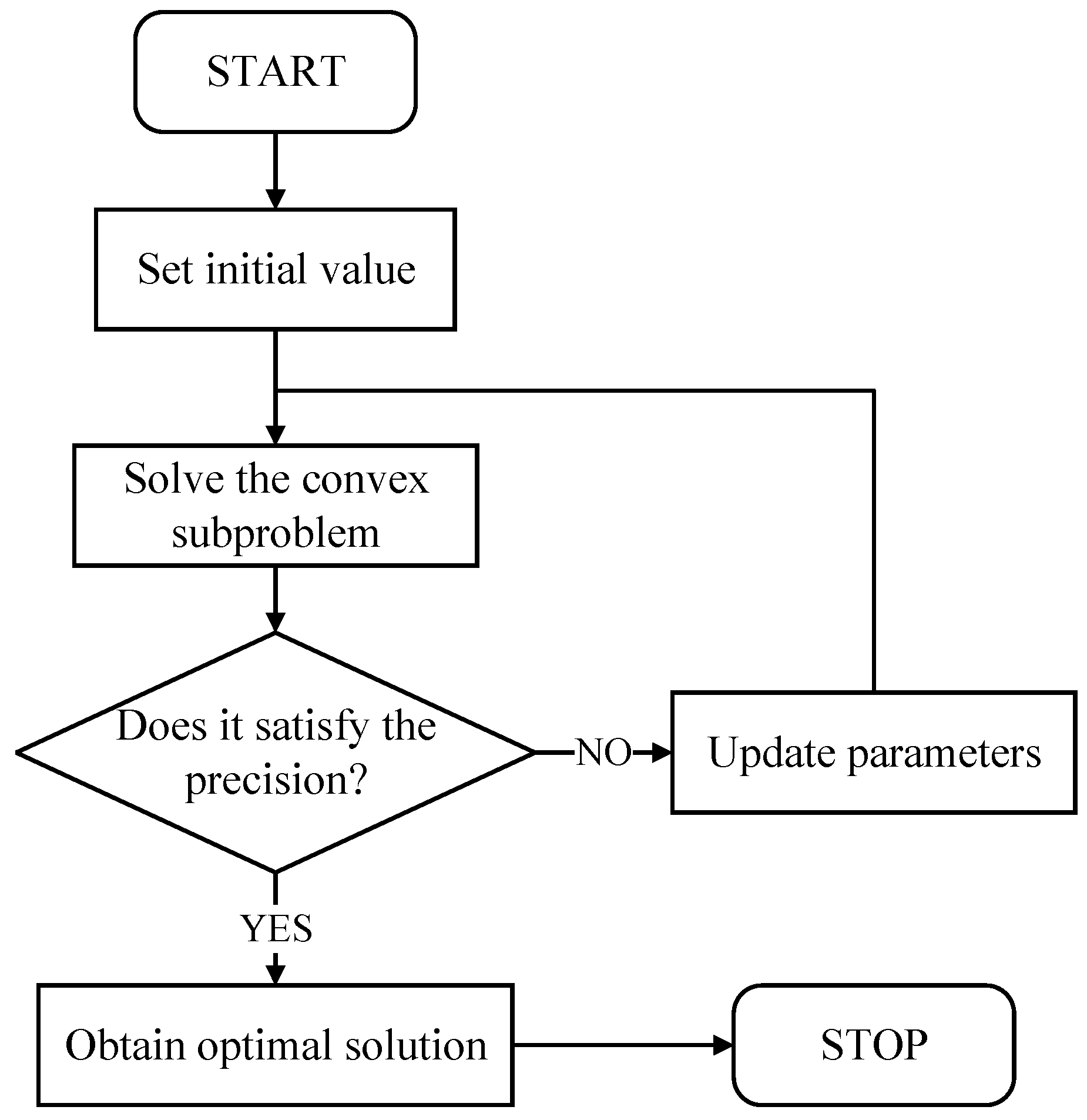
The solution procedure of the AL-CP-ISC to find the solution to the original problem is given. As shown in Figure 1, the convex subproblem can be solved iteratively until predetermined convergence precision is reached.

A more detailed solution procedure of the AL-CP-ISC algorithm is shown as follows (Algorithm 1):

Algorithm 1. AL-CP-ISC
1. Let $k=0$, set the initial reference trajectory ${\widehat{x}}^0$ by propagating the dynamical Equation (1) with the fixed control variables.
2. Assign initial values to the following parameters: penalty parameters $p_0$, penalty parameter update multiple ${\rho }_p>1$, initial Lagrange multipliers ${\lambda }_0,{\mu }_0$, initial trust region radius ${\delta }_0$, the iteration number of the trust region starts to update $k_{sc}$, the trust region contraction factor $0<b_0<1<b_1$, and the number of discrete points $N$.
3. $k\ge 1$, solve the convex subproblem $P_{SOCP}$ by the interior point method, and find solution pairs: ${\widehat{x}}^k={[x^k,u^k,t_f^k,{\zeta }_h^k,{\zeta }_g^k]}^T$.
4. Define the value of constraint violation $v$:
$v_k=\sqrt{{\displaystyle \sum {\zeta }_{i,h}^k·{\zeta }_{i,h}^k}+{\displaystyle \sum \left|\max \left({\zeta }_{i,g}^k,-{\mu }_i^{k-1}/p_{k-1}\right)\right|}}$	(30)
When $v_k\le \kappa$, go to 6, otherwise, go to 5, where $\kappa$ is a sufficiently small positive number.
5. Update penalty parameters  $p_k$ and Lagrange multipliers ${\lambda }_k,{\mu }_k$.
Then, $k=k+1$, and go to 3.
6. Obtain the optimal solution of the original problem:
${\widehat{x}}^{*}={[x^{*},u^{*},t_f^{*},{\zeta }_h^{*},{\zeta }_g^{*}]}^T={[x^k,u^k,t_f^k,{\zeta }_h^k,{\zeta }_g^k]}^T$.

Remark 1.

In Step 1, the initial reference trajectory generated by the numerical integration method meets the dynamic constraints, and the change in the bank angle and its rate are smooth. It is beneficial to enable linearization and facilitate the iteration. Nevertheless, notice that the quality of this initial trajectory may affect the convergence effect, such as the number of iterations and convergence accuracy. Therefore, taking into account factors such as the flight time, mission characters, and other constraint conditions, it is necessary to judiciously select the fixed control variable.

4. Numerical Verification

In this section, numerical simulations are employed to testify the effectiveness and convergence of the AL-CP-ISC algorithm. To compare with the simulation results of the AL-CP-ISC algorithm, CPM and P-CP-ISC algorithms are used to solve the same reentry trajectory optimization problem of the hypersonic vehicle. The CPM is the Chebyshev pseudo-spectral method that transforms the original problem into a general nonlinear programming problem and adopts the sequential quadratic programming algorithm to solve the problem. The difference between P-CP-ISC and AL-CP-ISC lies in different transformation approaches, and the objective function of the P-CP-ISC algorithm adopts the form of a penalty function without Lagrange multipliers.

According to Ref. [30], it is considered that the mass of the reentry vehicle is $m=104,035 \mathrm{kg}$, and the aerodynamic reference area is $S=391.22 {\mathrm{m}}^2$. In this paper, the fight mission of the vehicle is to plan an optimal trajectory with the minimum flight time under various constraints. Correspondingly, the initial and terminal constraints are: $h_0=100 \mathrm{km}$, ${\theta }_0=0^{\circ }$, ${\varphi }_0=0^{\circ }$, $V_0=7450 \mathrm{m}/\mathrm{s}$, ${\gamma }_0=-{0.5}^{\circ }$, ${\psi }_0=0^{\circ }$, ${\sigma }_0=1^{\circ }$, $h_f=25 \mathrm{km}$, ${\theta }_f={12}^{\circ }$, ${\varphi }_f={72}^{\circ }$, $500\le V_f\le 1500 \mathrm{m}/\mathrm{s}$, ${\gamma }_f=-{10}^{\circ }$, ${\psi }_f={90}^{\circ }$. The maximum values of the path constraints are ${\dot{Q}}_{\max }=1500 {\mathrm{kW}/\mathrm{m}}^2$, $q_{\max }=18,000 {\mathrm{N}/\mathrm{m}}^2$, and $n_{\max }=2.5g_0$, respectively. In addition, to keep enough control margin, the magnitude of the bank angle and bank angle rate are limited by $80{ }^{\circ }$ and $10{ }^{\circ }/s$. The longitude and latitude of the center of the NFZ constraint are ${\theta }_c=2^{\circ }$ and ${\varphi }_c={50}^{\circ }$, respectively, and the radius is about $222 \mathrm{km}$. The initial trust region size in Equation (26) is given as:

$${\delta }_0={[\frac{15000}{R_0},\frac{25\pi }{180},\frac{25\pi }{180},\frac{500}{V_0},\frac{25\pi }{180},\frac{25\pi }{180},\frac{25\pi }{180}]}^T.$$

In the solution procedure of the AL-CP-ISC algorithm, the termination condition is set to be $v_k\le {10}^{-9}$, and the number of CGL points is 80. In Step 1 of the algorithm procedure, the initial reference trajectory is generated by the numerical integration method, in which the fixed control variable is set to 0.015 $°/s$, and the estimated terminal time is 1610 s. All optimization algorithms in this section are implemented by MATLAB 2020b on a desktop computer equipped with Intel Core i7-10700K/3.80 GHz CPU. For the convex subproblems $P_{SOCP}$, the professional software MOSEK (Version 9. 3. 7.) [31] is used to solve them.

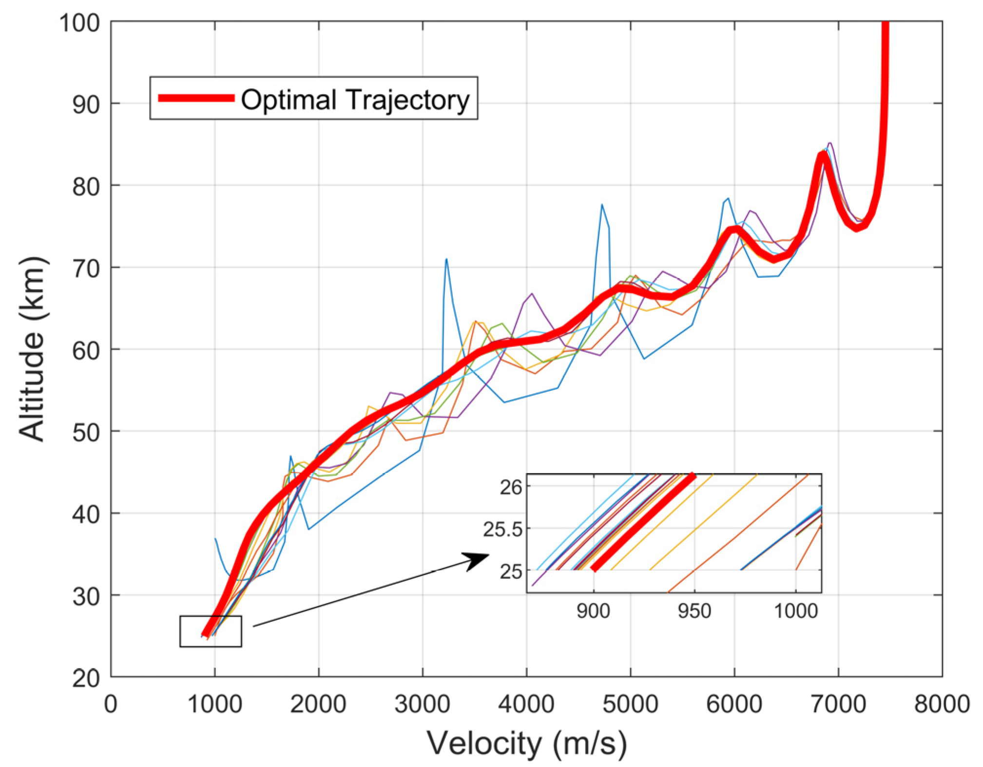
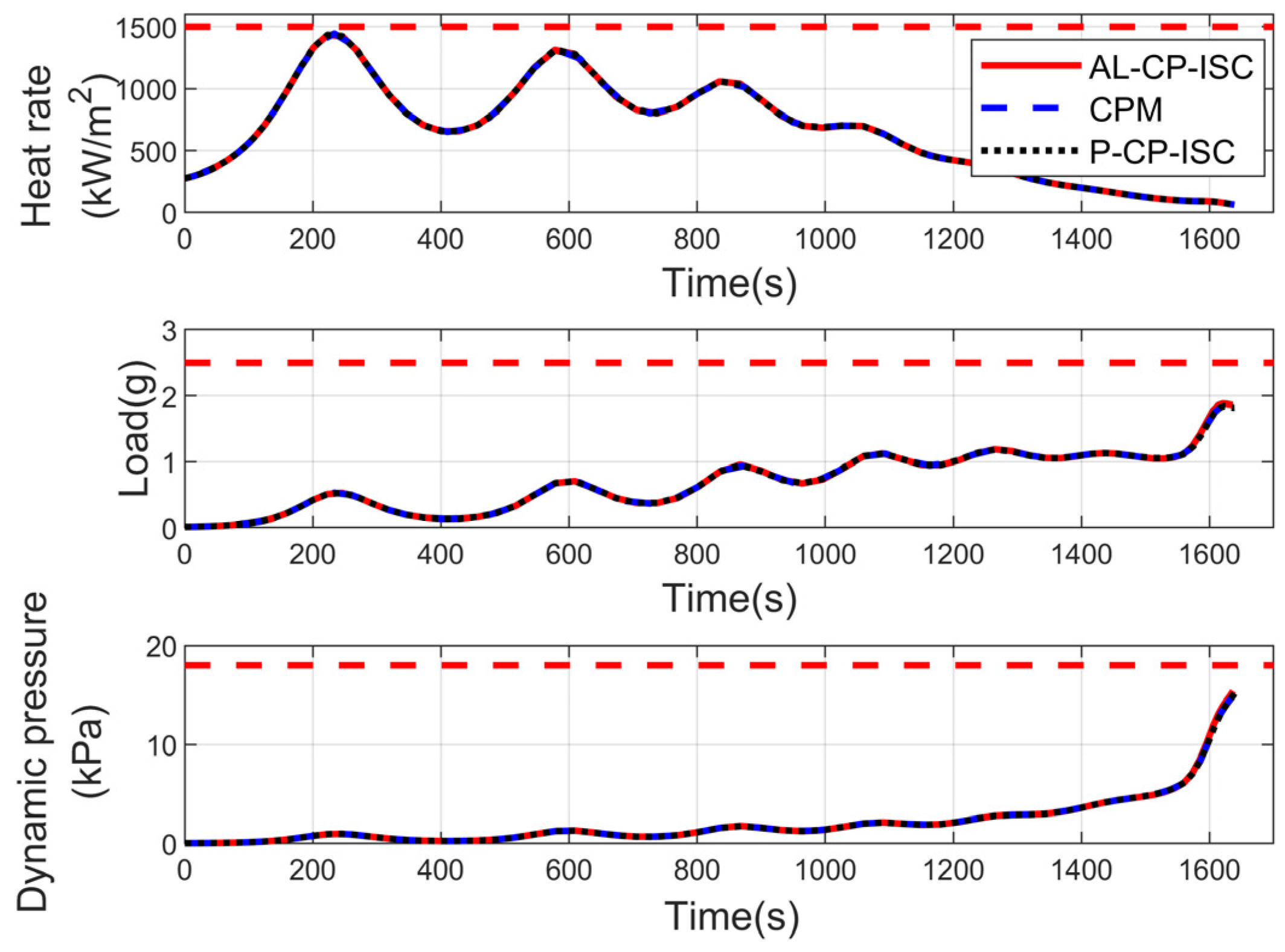
First, Figure 2, Figure 3, Figure 4, Figure 5, Figure 6 and Figure 7 present the trajectories of the vehicle obtained by the three algorithms, and

Table 1. Comparison of the simulation results.

Algorithm	Flight Time	${\mathit{h}}_{\mathit{f}}$	${\mathit{\theta }}_{\mathit{f}}$	${\mathit{\varphi }}_{\mathit{f}}$	${\mathit{V}}_{\mathit{f}}$	${\mathit{\gamma }}_{\mathit{f}}$	${\mathit{\psi }}_{\mathit{f}}$	Solve Time
CPM	1638.91 s	25 km	12 deg	72 deg	892.71 m/s	−10 deg	90 deg	287.8 s
AL-CP-ISC	1636.68 s	25 km	12 deg	72 deg	899.36 m/s	−10 deg	90 deg	4.20 s
P-CP-ISC	1638.94 s	25 km	12 deg	72 deg	892.63 m/s	−10 deg	90 deg	5.30 s

shows all the optimal solutions and solve time of each algorithm. The solid red curves are the solution of the AL-CP-ISC, the blue double lines represent the results of the CPM, and the other black dotted lines are the ones of the P-CP-ISC. In Figure 2, the profiles of each iteration of the AL-CP-ISC algorithm are depicted in different colors, from dark blue to warm red, to make the progression of the convergence clearer. The sequence solution converges in the 25th iteration, and the corresponding minimum flight time is 1636.68 s, which is quite close to the optimal solution from the other two algorithms. The trajectory curves almost overlap and are hard to distinguish in late iterations according to the zoom-in view. Moreover, Figure 3, Figure 4, Figure 5 and Figure 6 show a comparison of results between state variables and control variables, including altitude, velocity, longitude, latitude, flight-path angle, heading angle, bank angle, and its rate. It is obvious that all state and control profiles tend to be relatively consistent, and the initial, terminal, and bounded conditions required by the original problem are satisfied. In particular, it can be seen from Figure 4 that the trajectory of the vehicle successfully evades the no-fly zone. Meantime, the vehicle trajectories obtained by the three algorithms all meet the conditions of path constraints in Figure 7. In Table 1, in addition to the similar optimal solutions, it is worth noting that the solve time of AL-CP-ISC and P-CP-ISC is only 4.20 s and 5.30 s, far less than the solve time required by CPM. Given these analyses, it can be fully explained that the improvement measures of the sequential convexification algorithm do not affect the optimal solution, and the AL-CP-ISC algorithm can vastly reduce the computational cost; that is, the effectiveness and efficiency of the proposed algorithm are verified.

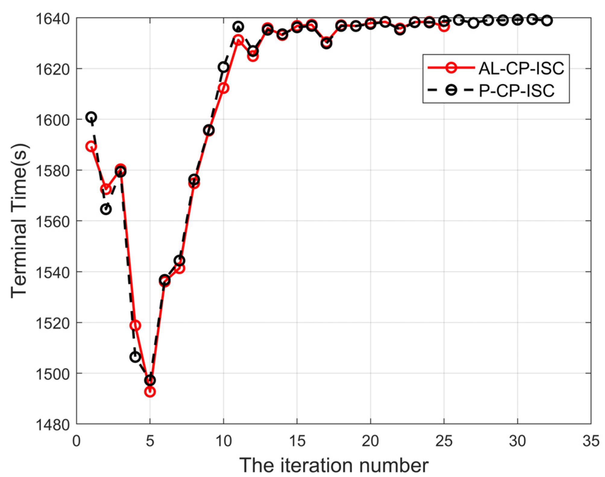
Then, the state trajectories of the AL-CP-ISC and P-CP-ISC algorithms are almost the same, and some slight differences are seen in the optimal flight time and the solve time. This shows that both algorithms can solve the approximate convex problem well. However, the number of iterations required by both algorithms is quite different according to Figure 8 and Figure 9, and they converge at the 25th and 32th iterations, respectively. Both figures are the value of constraint violations and the terminal flight time in each iteration, respectively. The only difference between the two algorithms is the form of the objective function. In a numerical sense, it indicates that the AL-CP-ISC algorithm with the augmented Lagrange function formal cost function has better convergence properties by comparing the trajectory results of these two algorithms.

5. Conclusions

In this paper, an improved sequential convexification algorithm is proposed to efficiently solve the trajectory planning problem of hypersonic vehicles based on the Chebyshev pseudo-spectral method and the method of multipliers. By employing the Chebyshev pseudo-spectral discretization method, the differential dynamical equations are transformed into the algebraic equation constraint. The original problem is then discretized into a finite-dimensional nonlinear programming problem. Next, through linearization and relaxation techniques, the slack variables, penalty parameters, and multipliers are introduced to transform the discrete problem into a series of relaxed convex subproblems in the form of the augmented Lagrange function, which are iteratively and efficiently solved by the MOSEK solver until the expected convergence precision is satisfied. The numerical simulation results verify the effectiveness, efficiency, and convergence performance of the proposed AL-CP-ISC algorithm. In the future, the proposed algorithm will be competitive for use in realizing onboard optimization due to its excellent optimization efficiency after code optimization.

References

- Betts, J.T. Survey of numerical methods for trajectory optimization. J. Guid. Control Dyn. 1998, 21, 193–207. [Google Scholar] [CrossRef]
- Chai, R.; Savvaris, A.; Tsourdos, A.; Chai, S.; Xia, Y. A review of optimization techniques in spacecraft flight trajectory design. Prog. Aerosp. Sci. 2019, 109, 100543. [Google Scholar] [CrossRef]
- Zhang, Y.; Zhang, R.; Li, H. Mixed-integer trajectory optimization with no-fly zone constraints for a hypersonic vehicle. Acta Astronaut. 2023, 207, 331–339. [Google Scholar] [CrossRef]
- Sagliano, M.; Mooij, E. Optimal drag-energy entry guidance via pseudospectral convex optimization. Aerosp. Sci. Technol. 2021, 117, 106946. [Google Scholar] [CrossRef]
- Wang, J.; Liang, H.; Qi, Z.; Ye, D. Mapped Chebyshev pseudospectral methods for optimal trajectory planning of differentially flat hypersonic vehicle systems. Aerosp. Sci. Technol. 2019, 89, 420–430. [Google Scholar] [CrossRef]
- Mao, Y.; Zhang, D.; Wang, L. Reentry trajectory optimization for hypersonic vehicle based on improved Gauss pseudospectral method. Soft Comput. 2017, 21, 4583–4592. [Google Scholar] [CrossRef]
- Zhou, H.; Wang, X.; Cui, N. Glide trajectory optimization for hypersonic vehicles via dynamic pressure control. Acta Astronaut. 2019, 164, 376–386. [Google Scholar] [CrossRef]
- Wang, J.; Cui, N.; Wei, C. Rapid trajectory optimization for hypersonic entry using a pseudospectral-convex algorithm. Proc. Inst. Mech. Eng. Part G J. Aerosp. Eng. 2019, 233, 5227–5238. [Google Scholar] [CrossRef]
- Wang, Z.; Grant, M.J. Constrained trajectory optimization for planetary entry via sequential convex programming. J. Guid. Control. Dyn. 2017, 40, 2603–2615. [Google Scholar] [CrossRef]
- Ma, Y.; Pan, B.; Hao, C.; Tang, S. Improved sequential convex programming using modified Chebyshev–Picard iteration for ascent trajectory optimization. Aerosp. Sci. Technol. 2022, 120, 107234. [Google Scholar] [CrossRef]
- Boris, B.; Alessandro, Z.; Guido, C.; Pizzurro, S.; Cavallini, E. Convex optimization of launch vehicle ascent trajectory with heat-flux and splash-down constraints. J. Spacecr. Rocket. 2022, 59, 900–915. [Google Scholar]
- Acikmese, B.; Ploen, S.R. Convex programming approach to powered descent guidance for mars landing. J. Guid. Control. Dyn. 2007, 30, 1353–1366. [Google Scholar] [CrossRef]
- Blackmore, L.; Açikmeşe, B.; Scharf, D.P. Minimum-landing-error powered-descent guidance for Mars landing using convex optimization. J. Guid. Control Dyn. 2010, 33, 1161–1171. [Google Scholar] [CrossRef]
- Wang, Z.; Grant, M.J. Optimization of minimum-time low-thrust transfers using convex programming. J. Spacecr. Rocket. 2018, 55, 586–598. [Google Scholar] [CrossRef]
- Lu, P.; Liu, X. Autonomous trajectory planning for rendezvous and proximity operations by conic optimization. J. Guid. Control Dyn. 2013, 36, 375–389. [Google Scholar] [CrossRef]
- Liu, X.; Lu, P. Robust trajectory optimization for highly constrained rendezvous and proximity operations. In Proceedings of the AIAA Guidance Navigation and Control (GNC) Conference, Boston, MA, USA, 15 August 2013; p. 4720. [Google Scholar]
- Wang, L.; Ye, D.; Xiao, Y.; Kong, X. Trajectory planning for satellite cluster reconfigurations with sequential convex programming method. Aerosp. Sci. Technol. 2023, 136, 108216. [Google Scholar] [CrossRef]
- Wang, J.; Cui, N.; Wei, C. Rapid trajectory optimization for hypersonic entry using convex optimization and pseudospectral method. Aircr. Eng. Aerosp. Technol. 2019, 91, 669–679. [Google Scholar] [CrossRef]
- Liu, X.; Shen, Z.; Lu, P. Entry trajectory optimization by second-order cone programming. J. Guid. Control Dyn. 2016, 39, 227–241. [Google Scholar] [CrossRef]
- Pei, P.; Fan, S.; Wang, W.; Lin, D. Online reentry trajectory optimization using modified sequential convex programming for hypersonic vehicle. IEEE Access 2021, 9, 23511–23525. [Google Scholar] [CrossRef]
- Fahroo, F.; Ross, I.M. Direct trajectory optimization by a Chebyshev pseudospectral method. J. Guid. Control Dyn. 2002, 25, 160–166. [Google Scholar] [CrossRef]
- Mittal, A.K.; Balyan, L.K. An improved pseudospectral approximation of coupled nonlinear partial differential equations. Int. J. Comput. Sci. Math. 2022, 15, 155–167. [Google Scholar] [CrossRef]
- Wang, Z.; Lu, Y. Improved sequential convex programming algorithms for entry trajectory optimization. J. Spacecr. Rocket. 2020, 57, 1373–1386. [Google Scholar] [CrossRef]
- Wang, Z. Optimal trajectories and normal load analysis of hypersonic glide vehicles via convex optimization. Aerosp. Sci. Technol. 2019, 87, 357–368. [Google Scholar] [CrossRef]
- Kanzow, C.; Nagel, C.; Kato, H.; Fukushima, M. Successive linearization methods for nonlinear semidefinite programs. Comput. Optim. Appl. 2005, 31, 251–273. [Google Scholar] [CrossRef]
- Nocedal, J.; Wright, S.J. Numerical Optimization; Springer: New York, NY, USA, 1999. [Google Scholar]
- Lu, Z.; Sun, Z.; Zhou, Z. Penalty and augmented Lagrangian methods for constrained DC programming. Math. Oper. Res. 2022, 47, 2260–2285. [Google Scholar] [CrossRef]
- Liu, X.-W.; Dai, Y.-H.; Huang, Y.-K.; Sun, J. A novel augmented Lagrangian method of multipliers for optimization with general inequality constraints. Math. Comput. 2023, 92, 1301–1330. [Google Scholar] [CrossRef]
- Liu, X.; Lu, P. Solving nonconvex optimal control problems by convex optimization. J. Guid. Control Dyn. 2014, 37, 750–765. [Google Scholar] [CrossRef]
- Stanley, D.O.; Engelund, W.C.; Lepsch, R.A.; McMillin, M.; Wurster, K.E.; Powell, R.W.; Guinta, T.; Unal, R. Rocket-powered single-stage vehicle configuration selection and design. J. Spacecr. Rocket. 1994, 31, 792–798. [Google Scholar] [CrossRef]
- Andersen, E.D.; Roos, C.; Terlaky, T. On implementing a primal-dual interior-point method for conic quadratic optimization. Math. Program. 2003, 95, 249–277. [Google Scholar] [CrossRef]
Figure 1.
Algorithm solution flow.
Figure 2.
Convergence of the trajectories using AL-CP-ISC.
Figure 3.
Comparison of altitude–velocity profile.
Figure 4.
Trajectories profile to avoid the NFZ.
Figure 5.
Comparison of fight-path angle and heading angle profile.
Figure 6.
Comparison of bank angle and bank angle rate profile.
Figure 7.
Comparison of the path constraints.
Figure 8.
Value of constraints violation for each iteration.
Figure 9.
Flight terminal time for each iteration.