
Semi-Analytical Closed-Form Solutions for Dynamical Rössler-Type System

1
Department of Mathematics, Politehnica University of Timisoara, 300006 Timisoara, Romania
2
Department of Physical Foundations of Engineering, Politehnica University of Timisoara, 300223 Timisoara, Romania
*
Author to whom correspondence should be addressed.
†
These authors contributed equally to this work.
Mathematics 2024, 12(9), 1308; https://doi.org/10.3390/math12091308
Submission received: 5 April 2024
/
Revised: 22 April 2024
/
Accepted: 23 April 2024
/
Published: 25 April 2024
(This article belongs to the Special Issue Analytical Approaches to Nonlinear Dynamical Systems and Applications II)
Abstract
:Mathematical models and numerical simulations are necessary to understand the functions of biological rhythms, to comprehend the transition from simple to complex behavior and to delineate the conditions under which they arise. The aim of this work is to investigate the Rssler-type system. This system could be proposed as a theoretical model for biological rhythms, generalizing this formula for chaotic behavior. It is assumed that the Rssler-type system has a Hamilton–Poisson realization. To semi-analytically solve this system, a Bratu-type equation was explored. The approximate closed-form solutions are obtained using the Optimal Parametric Iteration Method (OPIM) using only one iteration. The advantages of this analytical procedure are reflected through a comparison between the analytical and corresponding numerical results. The obtained results are in a good agreement with the numerical results, and they highlight that our procedure is effective, accurate and usefully for implementation in applicationssuch as an oscillator with cubic and harmonic restoring forces, the Thomas–Fermi equation and the Lotka–Voltera model with three species.
Keywords:
optimal parametric iteration method; dynamical system; symmetries; Hamilton–Poisson realization; periodical orbitsMSC:
37B65; 37C79; 65H20; 37J06; 37J35; 65L991. Introduction
Many applications in medicine, outdoor weather control applications, secure communication techniques and so on are based on the study of chaotic dynamic systems. This work explored a Bratu-type equation [1] to semi-analytically solve a Rssler-type system [2]. Various numerical methods use the Bratu problem as a test bed, and the generalization of this problem has led to the variety of applications in which it arises, such as radiative heat transfer, thermal reactions, chemical reactor theory, nanotechnology and so on.
Raja et al. [3] used the genetic algorithm (GA) and the active set method (ASM) to solve Bratu-type equations with applications in electrically conducting solids and various other physical phenomena. Caglar et al. [4] reported the dynamic behaviors of the solution of Bratu’s equation by computing the corresponding Lyapunov exponent, power spectra and cobweb diagrams modeling the chaotic regimes. Jalilian [5] obtained smooth approximate solutions using the non-polynomial spline method in comparison with those obtained using B-spline, Laplace and decomposition methods. Kafri et al. [6] developed an iterative algorithm combining Green’s function and fixed-point iterative schemes to solve the nonlinear Bratu’s boundary value problem. Hichar et al. [7] reported some solutions to this equation and its applications in electrostatics and plasma physics. Mohsen [8] discussed different iterative schemes, such as the finite-difference method and nonstandard finite-difference methods with a simple sinusoidal starting function, obtaining a simple solution for the Bratu problem. Wazwaz [9] applied the Adomian decomposition method to determine exact solutions for Bratu-type equations. Syam et al. [10] numerically solved Bratu’s equation using the Laplace–Adomain decomposition method. Boyd [11] built an analytical solution by using a series of even Chebyshev polynomials and comparing them with the corresponding numerical results obtained using the collocation or pseudospectral method. Abd et al. [12] applied some perturbation expansion methods to analytically solve the one-dimensional Bratu problem. Abbasbandy et al. [13] solved the Bratu equation using the Lie-group shooting method. Deniz et al. [14] proposed a new approach, namely the Optimal Perturbation Iteration Method, for solving Bratu-type problems. Keshavarz et al. [15] developed an efficient numerical method, namely the Taylor wavelet method, for obtaining analytical solutions for the Bratu-type equations. Abdelhakem et al. [16] solved some nonlinear problems using two spectral Legendre’s derivative algorithms. Singh et al. [17] adopted an efficient technique (the Haar wavelet method) for numerically solving Bratu-type equations. Mohsen [18] used Green’s function for obtaining the integral solution to Bratu’s equation. Temimi et al. [19] proposed a new computational scheme for the classical Bratu equation. Jator et al. [20] explored numerical solutions by applying the Block Nystrm Method. Behl et al. [21] presented a family of iterative methods to solve Bratu’s equation. Tomar et al. [22] introduced an efficient analytical iterative method that obtains a semi-analytical solution for the Bratu-type problem. Karamollahi et al. [23] used Hermite interpolation to approximate dual solutions for the strongly nonlinear one-dimensional Bratu problem. Jator et al. [24] introduced a new numerical scheme to solve Bratu’s problem. Singh et al. [25] applied the Homotopy Perturbation Method (HPM) to solve a class of Bratu’s equations. Aydinlik et al. [26] approached the Bratu-type equation based on the Smooth Composite Chebyshev Finite-Difference Method. Aksoy et al. [27] and obtained different perturbation–iteration solutions to the Bratu-type equations. Venkatesh et al. [28] used the Legendre wavelet method to solve Bratu-type initial value problems. Ragb et al. [29] introduced a numerical scheme based on differential quadrature methods for solving the Bratu problem. Masood et al. [30] tested Mexican Hat Wavelet neural networks for solving Bratu-type nonlinear systems. Ahmad et al. [31] proposed an efficient algorithm to obtain better solutions for Bratu differential equations.
Recently, Karimov et al. [32,33] proposed a novel technique by studying the synchronization between a circuit modeling the Rssler chaotic system. Ding et al. [34] investigated the existence of a Shilnikov-type homoclinic orbit of in the Rssler system and spiral chaos using the series expressions of the solution.
The impact of complex dynamic systems/nonlinear differential equations on real-world applications has led to the development of new mathematical methods for approaching dynamical behaviors and that consider the existence of chaos caused by the influence of several physical parameters. For example, Zhou [35] examined the asymptotic behavior of the Nicholson model with neutral-type delays, Zhou [36] studied a four-dimensional predator–prey chemostat model that considered the dynamical mechanism of cyclic persistence and the existence of periodic solutions. The difference between a classical and anomalous diffusion equation was analyzed by Zhao et al. [37].
Nonlinear wave dynamics, such as solitons, breathers, rogue waves and semi-rational solutions on periodic backgrounds, which are important for many physical systems, were investigated by Li et al. [38], who pointed out their dynamic behaviors.
In general, with chaotic systems, the exact solution can no longer be controlled, but their dynamic properties are analyzed with specific mathematical methods, such as bifurcation routes, Poincare maps, frequency spectra, amplitude modulation, topological horseshoes, the existence of a heteroclinic orbit or homoclinic orbit, equilibrium, Lyapunov exponent spectra, a dissipative system, phase portraits, bifurcation diagrams and Hopf bifurcation. These properties characterize the chaotic behaviors of dynamical systems.
The organization of the remainder of this paper is as follows. In Section 2, a short presentation of Bratu’s problem and the Rsller-type system is provided. Section 3 describes the Optimal Parametric Iteration Method and semi-analytical solutions. Section 4 contains the numerical results, and Section 5 summarizes the concluding remarks.
2. Preliminary
2.1. Bratu’s Problem
The original one-dimensional Bratu nonlinear boundary value problem is presented in [1]:
2.2. The Rsller-Type System
The Rsller-type system is written as follows [2]:
This subsection emphasizes the approximate closed-form solution of system (2) in the completely integrable case () studied in [40,41,42]:
System (3) is a Hamiltonian mechanical system with a Hamiltonian–Poisson structure characterized by the constants of motion given by
In considering the initial conditions
the exact solutions of Equations (3) and (5) are written as the intersection of the surfaces:
In taking into account Equation (4), it is more convenient to consider the following transformation:
which describes the closed-form solutions of Equations (3) and (5). The unknown smooth function u from Equation (7) is the solution of the nonlinear initial value problem
obtained from the first item of Equation (3).
The obtained problem given by Equation (8) is a Bratu-type nonlinear initial value problem with a linear control.
Section 3 presents some semi-analytical solutions of Equation (8) obtained using the OPIM procedure and that are denoted by or .
There are some analytical methods for solving nonlinear differential equations as follows: the optimal iteration parametrization method (OIPM) [43], the optimal homotopy asymptotic method (OHAM) [44,45,46], the optimal homotopy perturbation method (OHPM) [47,48,49] and the modified optimal parametric iteration method [50].
3. The Optimal Parametric Iteration Method
3.1. Preliminary
Some iteration procedures for solving different nonlinear problems were developed in [51,52,53,54,55].
The idea of the Optimal Parametric Iteration Method is to consider the following second-order nonlinear differential equation:
subject to the initial conditions
where is a linear operator; , a nonlinear operator; , a boundary operator; g, a known function; u, an unknown smooth function depending on the independent variable t; and .
For real values , and , by applying the well-known Taylor formula for an analytic function F, we obtain
where . Instead of solving nonlinear differential Equation (10), one can solve another equation, making recourse to Equation (12) and to the following scheme, namely, the Optimal Parametric Iteration Method (OPIM), introduced by Marinca et al. [43]:
where , and are auxiliary continuous functions; (obtained from the Taylor series expansion of the nonlinear operator ); is the (n + 1)-th-order approximate solution of Equations (10) and (11), denoted by or ; and is the initial approximation, a solution of the following linear differential problem:
The real constants , and are unknown convergence-control parameters and can be optimally computed.
The -order approximate solution of Equations (10) and (11) is well determined if the convergence-control parameters are known.
In the OPIM, the linear operator is arbitrarily chosen, not the physical parameters. There are situations when the choice of physical parameters give rise to the chaotic behavior of the dynamic system. This happens in the cases of choosing higher values for the damping factor or exceeding the optimal resonance conditions, as well as in the case of arbitrarily choosing the initial conditions.
If is the initial approximation of Equation (14), the nonlinear operators , , and that appear in Equation (13) have the form
where is a positive integer, and and are known functions that depend on .
For an -order approximate solution of Equations (10) and (11), the validation of this procedure is highlighted by computing the residual function given by
such that for all .
Using the linearly independent functions , we introduce some types of approximate solutions of Equation (10).
Definition 1.
The functions of the OPIM sequences are called OPIM functions of Equation (10).
The OPIM sequences with the property
are called convergent to the solution of Equation (10), where .
Definition 2.
The OPIM functions satisfying the conditions
are called ε-approximate OPIM solutions of Equation (10).
Definition 3.
The OPIM functions satisfying the conditions
are called weak ε-approximate OPIM solutions of Equation (10) on the real interval .
Remark 1.
The existence of weak -approximate OPIM solutions results from the theorem presented above.
Theorem 1.
Equation (10) admits a sequence of weak ε-approximate OPIM solutions.
Proof.
This is similar to the Theorem from [56].
Firstly, the OPIM sequences are built by considering the approximate OPIM solutions of the type
The unknown parameters , will be determined.
Upon introducing the approximate solutions into Equation (10), the expression yields
By attaching the real functional
to Equation (10) and imposing the initial conditions, we can determine , such that , , …, are computed as , , …, .
The values of , , …, are computed by replacing , , …, in Equation (21), which provide the minimum of functional (21).
By means of the initial conditions, the values , , …, as functions of , , …, are determined.
In using the constants , , …, thus determined, the following OPIM functions
are constructed.
The next step is to show that the above OPIM functions are weak -approximate OPIM solutions of Equation (10).
Therefore, the OPIM functions are computed, and in taking into account that the given by (20) are OPIM functions for Equation (10), it follows that
Thus,
Since is convergent to the solution of Equation (10), we obtain
It follows that for all , there exists such that for all and , the sequence is a weak -approximate OPIM solution of Equation (10). □
Remark 2.
The proof of the above theorem provides us a way to determine a weak ε-approximate OPIM solution of Equation (10), . Moreover, in taking into account Remark 1, if , then is also an ε-approximate OPIM solution of the considered equation.
Remark 3.
(1) The integration of Equation (13) produces secular terms of the forms , , , , , and so on. For the nonlinear oscillator, the secular terms that appear through integration generate the resonance phenomenon. Consequently, the secular terms have to be avoided.
(2) The OPIM method was successfully applied in the case of ODEs with boundary conditions, see Ref. [57], such as the following:
(a) A thin film flow of a fourth-grade fluid down a vertical cylinder:
where . The linear operator is chosen as .
(b) Thermal radiation on an MHD flow over a stretching porous sheet:
where the initial guess is chosen as and , with .
(c) An oscillator with cubic and harmonic restoring forces:
where linear operator is chosen as .
(d) The Thomas–Fermi equation:
where linear operator is chosen as , and the nonlinear operator yields .
(e) The Lotka–Voltera model with three species:
where the initial approximations are chosen as , and , or , and , and so on.
3.2. Semi-Analytical Solutions Using OPIM Technique
The applicability of the OPIM procedure for the nonlinear differential problems given by Equation (8) using only one iteration is presented in details below.
For obtaining a semi-analytical solution of Equation (8), it is more convenient to use the approximation in series:
In taking into consideration the linear operator given by Equation (28), the initial approximation , which is the solution of Equation (14), is
with .
In using Equation (28), a simple computation yields the following expressions:
In returning to Equation (13), there are a lot of possibilities to choose from for the following auxiliary functions:
or and so on.
In taking into account Equations (29) and (32), for , a simple integration of Equation (13), using only one iteration , yields
Neglecting secular terms yields
Therefore, for , the first approximation is a linear combination of the function set
where the parameters , , , and depending on the , and will be optimally identified.
In taking into account Equations (29) and (32), for , a simple integration of Equation (13), using only one iteration , yields
Neglecting secular terms yields
and so on.
Therefore, for , the first approximation is a linear combination of the function set
where the parameters , , , and depending on the , and will be optimally identified.
Generally, for a fixed number , the first approximation is a linear combination of the function set
where the parameters , , , and depending on the , and will be optimally identified.
Thus, in using only one iteration, the OPIM solution is well determined as by Equation (37).
Furthermore, using two iterations, the OPIM solution is computed as using Equation (37), and so on.
The initial conditions given by Equation (8) yield
4. Numerical Results and Validation
The Rssler-type system studied admits periodic solutions independently of the initial conditions, as it was proved in [2].
The results of the numerical study are provided in this section.
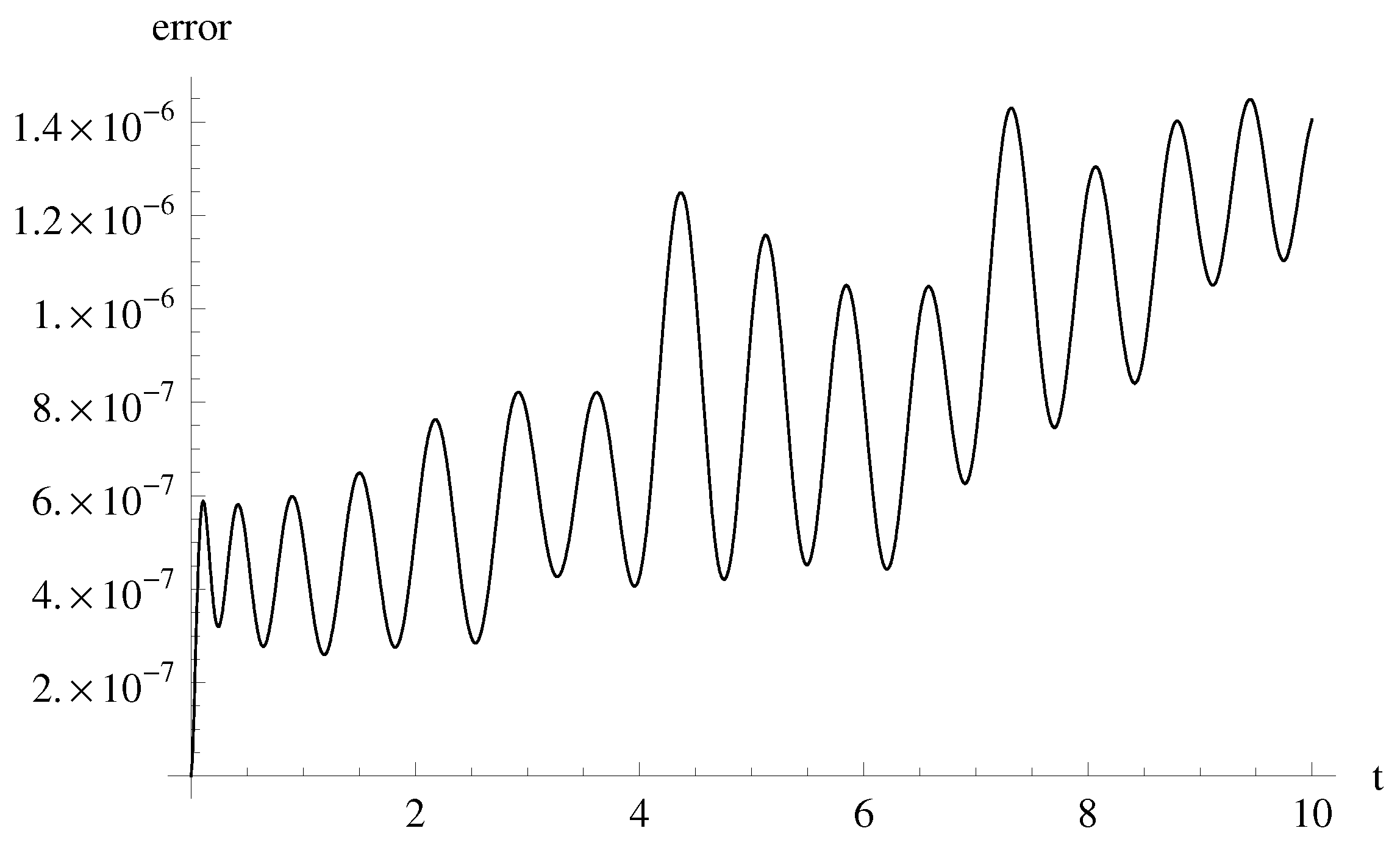
Firstly, the absolute errors are examined for different values of the index in Table 1 and Figure 1.
From Table 1, it can be observed that when the index increases, the magnitude of the absolute errors then decreases, until .
In choosing arbitrary values for the initial conditions , and , the profiles of the approximate analytic solutions , , and are represented in Figure 2 and Figure 3, highlighting the accuracy of the analytical procedure.
Comparisons between the semi-analytic closed-form solutions and and their corresponding numerical solutions are presented in Table 2 and Figure 2 and Table 3 and Figure 3, respectively. The precision and efficiency of the OPIM method (using just one iteration) compared to the iterative method described in [58] (using six iterations) are represented in Table 4 and Figure 4, respectively.
The profiles of the approximate analytic solution and each of , and have a periodic behavior, as depicted in Figure 2 and Figure 3.
The numerical values of the convergence-control parameters for for different values of the index are presented in detail in Appendix A.
OPIM Solutions versus Iterative Solutions
To emphasize the advantages of the presented method, the iterative solutions were obtained using the iterative method [58].
If system (3) is integrated over the interval , it results in the following:
The iterative procedure leads to the following:
The solutions of Equation (3), using the iterative algorithm, can be written as
The iterative solutions become the following after five iterations, when considering the initial conditions , and (presented in Table 4) and when taking into account algorithm (40):
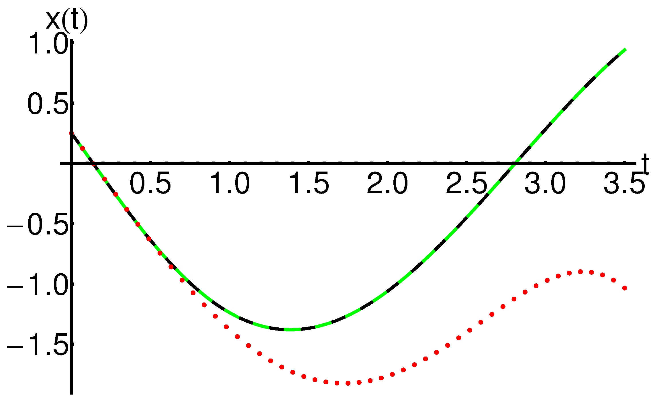
Figure 4 and Table 4, respectively, present a parallel between the OPIM solutions and the corresponding iterative solutions given in Equation (41). This comparative analysis highlights the efficiency and the accuracy of the modified OPIM method using only one iteration.
The improved precision and efficiency of the OPIM method (using just one iteration), compared to those of the iterative method described in [58] (using six iterations), are observed in the presented comparison.
The advantages of the OPIM method versus other methods are efficiency, convergence control (in the sense that the residual functions are smaller than 1), the non-existence of small parameters and the writing of the solutions in an effective form.
5. Conclusions
A new analytical approach, the OPIM, for solving second-order nonlinear differential equations was developed, which uses only one iteration.
The analytical approximate solutions were built for a class of nonlinear dynamical systems that possess a Hamilton–Poisson structure.
The obtained results were validated by graphically comparing them with the corresponding numerical solutions.
The accuracy of the results is illustrated through graphical and tabular representations.
These comparisons prove the precision of the applied method in the sense that the analytical solutions are approaching the exact solution.
The achieved results have high potential, and they encourage the study of dynamical systems with similar properties.
Author Contributions
Conceptualization, R.-D.E. and N.P.; methodology, N.P.; software, R.-D.E. and N.P.; validation, R.-D.E. and N.P.; formal analysis, R.-D.E. and N.P.; investigation, R.-D.E. and N.P.; writing—original draft preparation, R.-D.E. and N.P.; writing—review and editing, R.-D.E. and N.P.; visualization, R.-D.E. and N.P.; supervision, N.P. All authors have read and agreed on the published version of the manuscript.
Funding
Project number PFE 26/30.12.2021, PERFORM-CDI@UPT100-The increasing of the performance of the Polytechnic University of Timisoara by strengthening the research, development and technological transfer capacity in the field of “Energy, Environment and Climate Change” at the beginning of the second century of its existence, within Program 1-Development of the national system of Research and Development, Subprogram 1.2-Institutional Performance-Institutional Development Projects-Excellence Funding Projects in RDI, PNCDI III.
Data Availability Statement
No new data were created or analyzed in this study. Data sharing is not applicable to this article.
Acknowledgments
This work was supported by a grant of the Romanian Ministry of Research, Innovation and Digitalization, project number PFE 26/30.12.2021, PERFORM-CDI@UPT100-The increasing of the performance of the Polytechnic University of Timisoara by strengthening the research, development and technological transfer capacity in the field of “Energy, Environment and Climate Change” at the beginning of the second century of its existence, within Program 1-Development of the national system of Research and Development, Subprogram 1.2-Institutional Performance-Institutional Development Projects-Excellence Funding Projects in RDI, PNCDI III.
Conflicts of Interest
The authors declare no conflicts of interest.
Appendix A
References
- Bratu, G. Sur les equation integrals non-lineaires. Bull. Math. Soc. Fr. 1914, 42, 113–142. [Google Scholar] [CrossRef]
- Lazureanu, C.; Binzar, T. Some symmetries of a Rössler type system. Sci. Bull. Math.-Phys. 2013, 58, 1–6. [Google Scholar]
- Raja, M.A.Z.; Samar, R.; Alaidarous, E.S.; Shivanian, E. Bio-inspired computing platform for reliable solution of Bratu-type equations arising in the modeling of electrically conducting solids. Appl. Math. Model. 2016, 40, 5964–5977. [Google Scholar] [CrossRef]
- Caglar, H.; Caglar, N.; Özer, M.; Valaristos, A.; Miliou, A.N.; Anagnostopoulos, A.N. Dynamics of the solution of Bratu’s equation. Nonlinear Anal. 2009, 71, e672–e678. [Google Scholar] [CrossRef]
- Jalilian, R. Non-polynomial spline method for solving Bratu’s problem. Comput. Phys. Commun. 2010, 181, 1868–1872. [Google Scholar] [CrossRef]
- Kafri, H.Q.; Khuri, S.A. Bratu’s problem: A novel approach using fixed-point iterations and Green’s functions. Comput. Phys. Commun. 2016, 198, 97–104. [Google Scholar] [CrossRef]
- Hichar, S.; Guerfi, A.; Douis, S.; Meftah, M.T. Application of nonlinear Bratu’s equation in two and three dimensions to electrostatics. Rep. Math. Phys. 2015, 76, 283–290. [Google Scholar] [CrossRef]
- Mohsen, A. A simple solution of the Bratu problem. Comput. Math. Appl. 2014, 67, 26–33. [Google Scholar] [CrossRef]
- Wazwaz, A.-M. Adomian decomposition method for a reliable treatment of the Bratu-type equations. Appl. Math. Comput. 2005, 166, 652–663. [Google Scholar] [CrossRef]
- Syam, M.I.; Hamdan, A. An efficient method for solving Bratu equations. Appl. Math. Comput. 2006, 176, 704–713. [Google Scholar] [CrossRef]
- Boyd, J.P. One-point pseudospectral collocation for the one-dimensional Bratu equation. Appl. Math. Comput. 2011, 217, 5553–5565. [Google Scholar] [CrossRef]
- Abd-el-Malek, M.B.; Abdelrazek, A.; Ghazy, M.; Gamal, G. A modified perturbation solution to the one-dimensional Bratu problem. Appl. Math. Comput. 2019, 354, 296–304. [Google Scholar] [CrossRef]
- Abbasbandy, S.; Hashemi, M.S.; Liu, C.-S. The Lie-group shooting method for solving the Bratu equation. Commun. Nonlinear Sci. Numer. Simul. 2011, 16, 4238–4249. [Google Scholar] [CrossRef]
- Deniz, S.; Bildik, N. Optimal perturbation iteration method for Bratu-type problems. J. King Saud Univ.-Sci. 2018, 30, 91–99. [Google Scholar] [CrossRef]
- Keshavarz, E.; Ordokhani, Y.; Razzaghi, M. The Taylor wavelets method for solving the initial and boundary value problems of Bratu-type equations. Appl. Numer. Math. 2018, 128, 205–216. [Google Scholar] [CrossRef]
- Abdelhakem, M.; Youssri, Y.H. Two spectral Legendre’s derivative algorithms for Lane-Emden, Bratu equations, and singular perturbed problems. Appl. Numer. Math. 2021, 169, 243–255. [Google Scholar] [CrossRef]
- Singh, S.M.; Singh, K. An advancement approach of Haar wavelet method and Bratu-type equations. Appl. Numer. Math. 2021, 170, 74–82. [Google Scholar]
- Mohsen, A. On the integral solution of the one-dimensional Bratu problem. J. Comput. Appl. Math. 2013, 251, 61–66. [Google Scholar] [CrossRef]
- Temimi, H.; Ben-Romdhane, M. An iterative finite difference method for solving Bratu’s problem. J. Comput. Appl. Math. 2016, 292, 76–82. [Google Scholar] [CrossRef]
- Jator, S.N.; Manathunga, V. Block Nyström type integrator for Bratu’s equation. J. Comput. Appl. Math. 2018, 327, 341–349. [Google Scholar] [CrossRef]
- Behl, R.; Sarría, Í.; González, R.; Magreñán, Á.A. Highly efficient family of iterative methods for solving nonlinear models. J. Comput. Appl. Math. 2019, 346, 110–132. [Google Scholar] [CrossRef]
- Tomar, S.; Pandey, R.K. An efficient iterative method for solving Bratu-type equations. J. Comput. Appl. Math. 2019, 357, 71–84. [Google Scholar] [CrossRef]
- Karamollahi, N.; Loghmani, G.B.; Heydari, M. A computational method to find dual solutions of the one-dimensional Bratu problem. J. Comput. Appl. Math. 2021, 388, 113309. [Google Scholar] [CrossRef]
- Jator, S.N.; Mayo, D.C.; Omojola, M.T. Block Hybrid Third Derivative Nyström type Method for Bratu’s equation. Math. Comput. Simul. 2021, 185, 256–271. [Google Scholar] [CrossRef]
- Jyoti; Singh, M. An iterative technique based on HPM for a class of one dimensional Bratu’s type problem. Math. Comput.Simul. 2022, 200, 50–64. [Google Scholar] [CrossRef]
- Aydinlik, S.; Kiris, A.; Roul, P. An effective approach based on Smooth Composite Chebyshev Finite Difference Method and its applications to Bratu–type and higher order Lane–Emden problems. Math. Comput. Simul. 2022, 202, 193–205. [Google Scholar] [CrossRef]
- Aksoy, Y.; Pakdemirli, M. New perturbation-iteration solutions for Bratu–type equations. Comput. Math. Appl. 2010, 59, 2802–2808. [Google Scholar] [CrossRef]
- Venkatesh, S.G.; Ayyaswamy, S.K.; Balachandar, S.R. The Legendre wavelet method for solving initial value problems of Bratu–type. Comput. Math. Appl. 2012, 63, 1287–1295. [Google Scholar] [CrossRef]
- Ragb, O.; Seddek, L.F.; Matbuly, M.S. Iterative differential quadrature solutions for Bratu problem. Comput. Math. Appl. 2017, 74, 249–257. [Google Scholar] [CrossRef]
- Masood, Z.; Majeed, K.; Samar, R.; Zahoor Raja, M.A. Design of Mexican Hat Wavelet neural networks for solving Bratu type nonlinear systems. Neurocomputing 2017, 221, 1–14. [Google Scholar] [CrossRef]
- Ahmad, A.; Sulaiman, M.; Aljohani, A.J.; Alhindi, A.; Alrabaiah, H. Design of an efficient algorithm for solution of Bratu differential equations. Ain Shams Eng. J. 2021, 12, 2211–2225. [Google Scholar] [CrossRef]
- Karimov, A.I.; Rybin, V.G.; Kopets, E.E.; Karimov, T.I.; Nepomuceno, E.; Butusov, D. Identifying empirical equations of chaotic circuit from data. Nonlinear Dynam. 2023, 111, 871–886. [Google Scholar] [CrossRef]
- Karimov, A.; Tutueva, A.; Karimov, T.; Druzhina, O.; Butusov, D. Adaptive generalized synchronization between circuit and computer implementations of the Rössler system. Appl. Sci. 2021, 11, 81. [Google Scholar] [CrossRef]
- Ding, Y.; Zheng, L. Existence of homoclinic orbit of Shilnikov type and the application in Rössler system. Math. Comput. Simul. 2023, 206, 770–779. [Google Scholar] [CrossRef]
- Zhou, H. Dynamical behavior of almost periodically forced neutral delayed equation and its applications. Proc. Am. Math. Soc. 2022, 150, 5293–5309. [Google Scholar] [CrossRef]
- Zhou, H. Analysis of a mathematical model arising from stage-structured predator-prey in a chemostat. Nonlinear Anal.-Real World Appl. 2024, 77, 104031. [Google Scholar] [CrossRef]
- Zhao, Y.; Tang, Y. Critical behavior of a semilinear time fractional diffusion equation with forcing term depending on time and space. Chaos Solitons Fract. 2024, 178, 114309. [Google Scholar] [CrossRef]
- Li, X.-L.; Guo, R. Interactions of Localized Wave Structures on Periodic Backgrounds for the Coupled Lakshmanan-Porsezian-Daniel Equations in Birefringent Optical Fibers. Ann. Phys. 2023, 535, 2200472. [Google Scholar] [CrossRef]
- Ascher, U.M.; Mattheij, R.M.M.; Russell, R.D. Numerical Solution of Boundary Value Problems for Ordinary Differential Equations; SIAM: Philadelphia, PA, USA, 1995. [Google Scholar]
- Lima, M.F.S.; Llibre, J. Global dynamics of the Rössler system with conserved quantities. J. Phys. A Math. Theor. 2011, 44, 365201. [Google Scholar] [CrossRef]
- Llibre, J.; Zhang, X. Darboux integrability for the Rössler system. Int. J. Bifurc. Chaos Appl. Sci. Eng. 2002, 12, 421–428. [Google Scholar] [CrossRef]
- Tudoran, R.M.; Girban, A. On some asymptotic properties of the Rössler dynamical system. Stud. Univ. Babes-Bolyai Math. 2013, 58, 503–509. [Google Scholar]
- Marinca, V.; Draganescu, G.E. Construction of approximate periodic solutions to a modified van der Pol oscillator. Nonlinear Anal.-Real World Appl. 2010, 11, 4355–4362. [Google Scholar] [CrossRef]
- Herisanu, N.; Marinca, V. Accurate analytical solutions to oscillators with discontinuities and fractional-power restoring force by means of the optimal homotopy asymptotic method. Comput. Math. Appl. 2010, 60, 1607–1615. [Google Scholar] [CrossRef]
- Marinca, V.; Herisanu, N. The Optimal Homotopy Asymptotic Method—Engineering Applications; Springer: Berlin/Heidelberg, Germany, 2015. [Google Scholar]
- Marinca, V.; Herisanu, N. An application of the optimal homotopy asymptotic method to Blasius problem. Rom. J. Tech. Sci. Appl. Mech. 2015, 60, 206–215. [Google Scholar]
- Marinca, V.; Herisanu, N. Nonlinear dynamic analysis of an electrical machine rotor-bearing system by the optimal homotopy perturbation method. Comput. Math. Appl. 2011, 61, 2019–2024. [Google Scholar] [CrossRef]
- Marinca, V.; Ene, R.D.; Marinca, B. Optimal Homotopy Perturbation Method for nonlinear problems with applications. Appl. Comput. Math. 2022, 21, 123–136. [Google Scholar]
- Ene, R.D.; Pop, N. Semi-Analytical Closed-Form Solutions for the Rikitake-Type System through the Optimal Homotopy Perturbation Method. Mathematics 2023, 11, 3078. [Google Scholar] [CrossRef]
- Ene, R.D.; Pop, N. Approximate Closed-Form Solutions for a Class of Dynamical Systems involving a Hamilton-Poisson Part. Mathematics 2023, 11, 4811. [Google Scholar] [CrossRef]
- Mickens, R.E. Iteration procedure for determining approximate solutions to nonlinear oscillation equations. J. Sound Vib. 1987, 116, 185–188. [Google Scholar] [CrossRef]
- Mickens, R.E. A generalized iteration procedure for calculating approximations to periodic solutions of “truly nonlinear oscillators”. J. Sound Vib. 2005, 287, 1045–1051. [Google Scholar] [CrossRef]
- Lim, C.W.; Wu, B.S. A modified procedure for certain non-linear oscillators. J. Sound Vib. 2002, 257, 202–226. [Google Scholar] [CrossRef]
- Hu, H. Solutions of a quadratic nonlinear oscillator: Iteration procedure. J. Sound Vib. 2006, 298, 1159–1165. [Google Scholar] [CrossRef]
- Chen, Y.M.; Liu, J.K. A modified Mickens iteration procedure for nonlinear oscillators. J. Sound Vib. 2008, 314, 465–473. [Google Scholar] [CrossRef]
- Ene, R.D.; Pop, N.; Lapadat, M.; Dungan, L. Approximate closed-form solutions for the Maxwell-Bloch equations via the Optimal Homotopy Asymptotic Method. Mathematics 2022, 10, 4118. [Google Scholar] [CrossRef]
- Marinca, V.; Herisanu, N. Nonlinear Dynamical Systems in Engineering; Springer: Berlin/Heidelberg, Germany, 2011. [Google Scholar]
- Daftardar-Gejji, V.; Jafari, H. An iterative method for solving nonlinear functional equations. J. Math. Anal. Appl. 2006, 316, 753–763. [Google Scholar] [CrossRef]
Figure 1.
Profile of the absolute errors: for initial conditions , , and ; the analytic approximate solution of Equation (8) obtained from Equations (37), (38) and (A4).

Figure 2.
Profile of the approximate analytic solution of Equation (8) obtained from Equations (37), (38) and (A4) for initial conditions , , and ; OPIM solution (dotted line) and numerical solution (solid line).
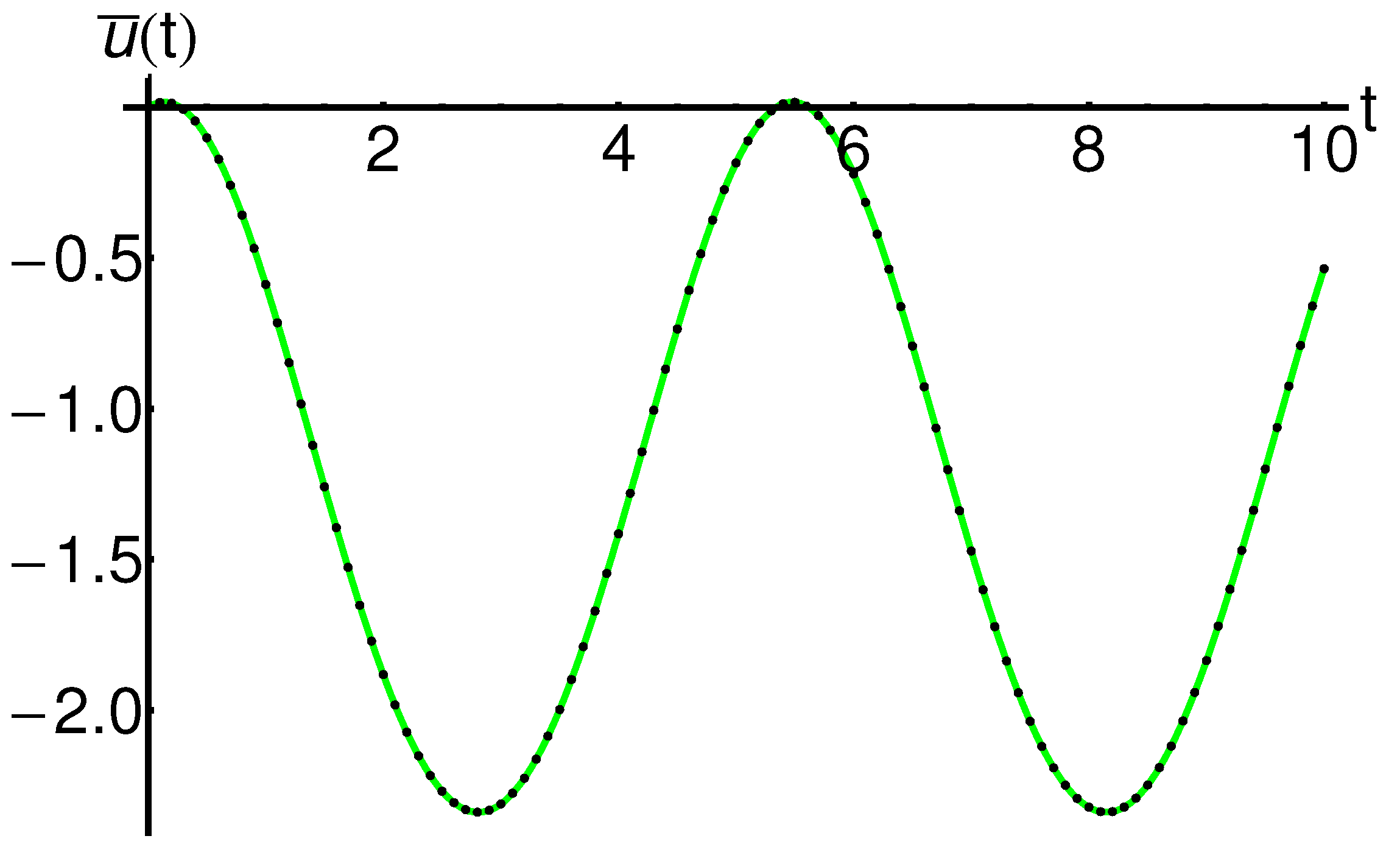
Figure 3.
Profile of the closed-form solutions , and given by Equations (9) and (A4) for initial conditions , , and ; OPIM solution (dotted line) and numerical solution (solid line).
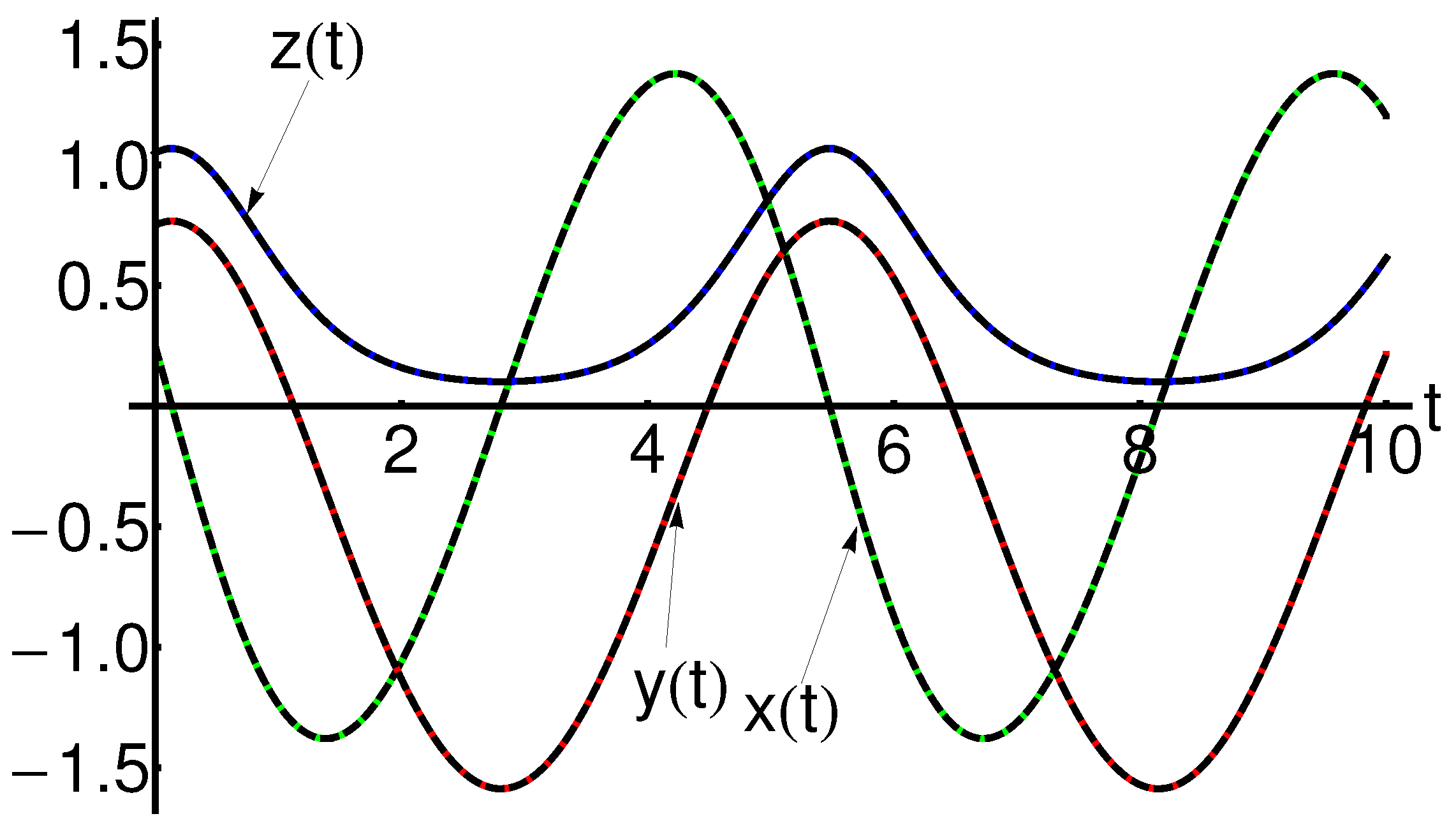
Figure 4.
Profiles of the approximate analytical solution of Equation (3) given by Equation (A4), the iterative solution given by Equation (41) and the corresponding numerical solution; OPIM solution (dashed black line), iterative solution (dotted red line) and numerical solution (solid green line).

Table 1.
Values of the absolute errors: for initial conditions , and and different values of the index ; analytic approximate solution of Equation (8) obtained from Equations (37), (38) and (A1)–(A4).
| t | ||||
|---|---|---|---|---|
| 0 | 5.68434 × | 8.12291 | 4.54747 | 7.10543 |
| 1/2 | 1.56141 | 8.68649 | 2.21405 | 4.85037 |
| 1 | 1.48405 | 1.41248 | 2.6783 | 5.0592 |
| 3/2 | 6.04191 | 3.44 | 1.44322 | 6.4853 |
| 2 | 3.3371 | 9.82754 | 3.82636 | 5.22813 |
| 5/2 | 6.32447 | 3.4972 | 3.48186 | 2.96143 |
| 3 | 3.62685 | 1.43278 | 7.30771 | 7.67939 |
| 7/2 | 4.35175 | 4.90013 | 7.79294 | 7.20673 |
| 4 | 4.14164 | 1.68089 | 1.48269 | 4.27381 |
| 9/2 | 3.19588 | 1.68538 | 2.11227 | 1.03521 |
| 5 | 1.32596 | 1.90962 | 2.91648 | 9.71333 |
| 11/2 | 1.90914 | 3.46814 | 1.51662 | 4.52946 |
| 6 | 1.3966 | 2.01006 | 3.01251 | 8.10717 |
| 13/2 | 3.33686 | 8.48484 | 4.2035 | 9.86731 |
| 7 | 1.15607 | 1.38123 | 8.79764 | 7.25709 |
| 15/2 | 3.18879 | 9.57228 | 2.69659 | 1.10401 |
| 8 | 5.01597 | 1.00957 | 5.19338 | 1.25896 |
| 17/2 | 6.856 | 5.66887 | 2.75871 | 9.05699 |
| 9 | 3.01073 | 5.25215 | 5.99213 | 1.1485 |
| 19/2 | 6.08924 | 1.05709 | 6.60261 | 1.42172 |
| 10 | 4.58559 | 2.81366 | 1.80462 | 1.40391 |
Table 2.
The approximate analytic solution of Equation (8) given by Equations (37) and (38) and the corresponding numerical solution for initial conditions , , and the index (absolute errors: ).
| t | |||
|---|---|---|---|
| 0 | −8.12291 | −7.10542 | 7.10542 |
| 1/2 | −0.1009833721 | −0.1009828870 | 4.85037 |
| 1 | −0.5875537666 | −0.5875532607 | 5.05920 |
| 3/2 | −1.2588228636 | −1.2588222150 | 6.48530 |
| 2 | −1.8816621245 | −1.8816616017 | 5.22813 |
| 5/2 | −2.2683521270 | −2.2683518309 | 2.96142 |
| 3 | −2.3108289294 | −2.3108281614 | 7.67938 |
| 7/2 | −1.9975070462 | −1.9975063255 | 7.20673 |
| 4 | −1.4151229407 | −1.4151225133 | 4.27380 |
| 9/2 | −0.7351867600 | −0.7351857248 | 1.03520 |
| 5 | −0.1849885987 | −0.1849876273 | 9.71333 |
Table 3.
The approximate analytic solution given by Equation (9) and corresponding numerical solution for initial conditions , , and the index (absolute errors: ).
Table 3.
The approximate analytic solution given by Equation (9) and corresponding numerical solution for initial conditions , , and the index (absolute errors: ).
| t | |||
|---|---|---|---|
| 0 | 0.25 | 0.2499999249 | 7.50267 |
| 1/2 | −0.6367781227 | −0.6367801438 | 2.02113 |
| 1 | −1.2376076804 | −1.2376093968 | 1.71634 |
| 3/2 | −1.3673785582 | −1.3673786474 | 8.91577 |
| 2 | −1.0603932046 | −1.0603910929 | 2.11171 |
| 5/2 | −0.4497705143 | −0.4497711768 | 6.62540 |
| 3 | 0.2837908478 | 0.2837896153 | 1.23259 |
| 7/2 | 0.9401129558 | 0.9401146702 | 1.71439 |
| 4 | 1.3313637430 | 1.3313651699 | 1.42692 |
| 9/2 | 1.3107276683 | 1.3107251137 | 2.55464 |
| 5 | 0.8126645233 | 0.8126672218 | 2.69845 |
Table 4.
Values of the approximate analytical solution (A4), the iterative solution Equation (41) and the corresponding numerical solution.
| t | |||
|---|---|---|---|
| 0 | 0.25 | 0.2499999249 | 0.25 |
| 0.35 | −0.3847286943 | −0.3847266999 | −0.3823724677 |
| 0.7 | −0.9282966040 | −0.9282953550 | −0.9683700083 |
| 1.05 | −1.2724487484 | −1.2724506529 | −1.4370077000 |
| 1.4 | −1.3794335466 | −1.3794320704 | −1.7324569333 |
| 1.75 | −1.2616050449 | −1.2616062739 | −1.8234993489 |
| 2.1 | −0.9572932068 | −0.9572918609 | −1.7129807750 |
| 2.45 | −0.5195989669 | −0.5196005038 | −1.4472651645 |
| 2.8 | −0.0116471526 | −0.0116453617 | −1.1256885333 |
| 3.15 | 0.4978649029 | 0.4978635857 | −0.9100128968 |
| 3.5 | 0.9401129558 | 0.9401146702 | −1.0338802083 |
Disclaimer/Publisher’s Note: The statements, opinions and data contained in all publications are solely those of the individual author(s) and contributor(s) and not of MDPI and/or the editor(s). MDPI and/or the editor(s) disclaim responsibility for any injury to people or property resulting from any ideas, methods, instructions or products referred to in the content. |
© 2024 by the authors. Licensee MDPI, Basel, Switzerland. This article is an open access article distributed under the terms and conditions of the Creative Commons Attribution (CC BY) license (https://creativecommons.org/licenses/by/4.0/).
Share and Cite
MDPI and ACS Style
Ene, R.-D.; Pop, N. Semi-Analytical Closed-Form Solutions for Dynamical Rössler-Type System. Mathematics 2024, 12, 1308. https://doi.org/10.3390/math12091308
AMA Style
Ene R-D, Pop N. Semi-Analytical Closed-Form Solutions for Dynamical Rössler-Type System. Mathematics. 2024; 12(9):1308. https://doi.org/10.3390/math12091308
Chicago/Turabian StyleEne, Remus-Daniel, and Nicolina Pop. 2024. "Semi-Analytical Closed-Form Solutions for Dynamical Rössler-Type System" Mathematics 12, no. 9: 1308. https://doi.org/10.3390/math12091308
Note that from the first issue of 2016, this journal uses article numbers instead of page numbers. See further details here.