
Deep Learning Based Fall Recognition and Forecasting for Reconfigurable Stair-Accessing Service Robots
by
 , , and
Jun Hua Ong
1,
Abdullah Aamir Hayat
1,*,
Braulio Felix Gomez
1,
Mohan Rajesh Elara
1 and
Kristin Lee Wood
2 1
Robotics and Automation Research (ROAR) Lab, Engineering Product Development Pillar, Singapore University of Technology and Design (SUTD), Singapore 487372, Singapore
2
College of Engineering, Design and Computing, University of Colorado Denver, 1200 Larimer St, Ste. 3034, Denver, CO 80204, USA
*
Author to whom correspondence should be addressed.
Mathematics 2024, 12(9), 1312; https://doi.org/10.3390/math12091312
Submission received: 18 February 2024
/
Revised: 16 April 2024
/
Accepted: 23 April 2024
/
Published: 25 April 2024
Abstract
:This paper presents a comprehensive study on fall recognition and forecasting for reconfigurable stair-accessing robots by leveraging deep learning techniques. The proposed framework integrates machine learning algorithms and recurrent neural networks (RNNs), specifically Long Short-Term Memory (LSTM) and Bidirectional LSTM (BiLSTM), for fall detection of service robots on staircases. The reconfigurable stair-accessing robot sTetro serves as the platform, and the fall data required for training models are generated in a simulation environment. The two machine learning algorithms are compared and their effectiveness on the fall recognition task is reported. The results indicate that the BiLSTM model effectively classifies falls with a median categorical accuracy of 94.10% in simulation and 90.02% with limited experiments. Additionally, the BiLSTM model can be used for forecasting, which is practically valuable for making decisions well before the onset of a free fall. This study contributes insights into the design and implementation of fall detection systems for service robots used to navigate staircases through deep learning approaches. Our experimental and simulation data, along with the simulation steps, are available for reference and analysis via the shared link.
Keywords:
reconfigurable robots; deep learning; fall detection; design principles; recurrent neural network; LSTM; BiLSTM; service robotsMSC:
68T40; 68T071. Introduction
Staircase-cleaning robots represent a significant advancement in robotics for facility maintenance. Cleaning robots form a major sector of the commercial robots in use today, with a global market valued at USD 8.34 billion in 2021 and a compound annual growth rate of 22.7% [1]. Among cleaning robots, floor cleaning robots are the most common [2]; however, conventional floor cleaning robots are unable to handle staircase environments. One reason staircase robots in general are rare and commercial staircase cleaning robots nonexistent is that staircases represent a risky operating environment. Robots are susceptible to falls caused by collisions with people or objects as well as from errors in movement resulting in a loss of balance. In a case where a robot falls from the staircase, it will likely slide or tumble down the stairs, causing severe damage to the robotic system and anything in its path. The inherent risk and large impact of falls during operation necessitates the development of intelligent systems capable of fall recognition and prediction to ensure the safety of the robot, prevent damage to the surroundings, and mitigate potential injuries to people nearby.
In studying falls, whether for robots or humans, accurate detection, classification, and forecasting are crucial. Detection involves identifying the occurrence of a fall event or the presence of specific incidents in a given context, i.e., detecting whether a fall has happened based on sensor data or environmental cues. Wang et al. [3] detailed various fall detection technologies and reported their sensitivity and accuracy. Classification refers to assigning a label or category to a fall event based on predefined classes, for example, backward/forward falls, left/right leaning falls, and slip/spin falls. In Kerdjidj et al. [4], human activities such as sitting, running, standing, and falling were classified based on data from wearable sensors. Forecasting or prediction refers to foreseeing future fall events based on historical data or patterns. One example is the gait-based human fall prediction model using deep learning approach employed in Sampath et al. [5]. The significance of fall recognition lies in its ability to trigger appropriate responses and mechanisms to mitigate damage caused by falls. This paper further explores fall detection, classification, and forecasting along with their application in the context of a service robot employed in staircase cleaning.
Fall prediction and forecasting are widely studied topics for bipedal robots. This is due to the inherent imbalance arising from their smaller support base (footprint) and higher center of gravity compared to other robot types. Two main approaches are used to predict falls for these robots: the inverted pendulum model, and machine learning approaches. An example of the inverted pendulum model is the Energy-based Fall Prediction (EFP) method developed in [6]. This method provides an analytical and quantitative measure of balance by monitoring the robot’s state in real time. Studies have shown that EFP can successfully predict falls about 0.3 s in advance, outperforming other indicators such as Capture Point (CP) and Foot Rotation Indicator (FRI) in both simulated and real-world scenarios. Previous studies have explored various strategies for fall avoidance and recovery in bipedal robots, including the use of walking sticks as proposed in [7] and model-based approaches for fall detection and prevention in [8]. However, by using fall data and applying supervised learning methods, researchers aim to achieve more reliable fall prediction, with experiments on ASIMO-like robots showing promising results [9]. To mitigate this risk, machine learning-based fall detection methods have been proposed, requiring minimal training data and utilizing support vector machines to enhance detection accuracy [10,11]. In short, the training data are essential for machine learning approaches, whereas a model-based approach such as inverted pendulum does not require extensive data for modeling.
The use of synthetic IMU data generated with biomechanical simulations was used to address limitations in acquiring real fall data for machine learning-based fall detection in [12]. Despite these advancements, challenges remain in acquiring sufficient and diverse fall data for training robust machine learning models as well as in ensuring the generalizability of these models across different robot platforms and environments. Additionally, the complex dynamics and unpredictability of human movements pose challenges for accurate fall prediction in real-time scenarios. These challenges underscore the importance of continued research efforts to develop more reliable fall prediction methods for a given robot design operating in a given environment.
Moreover, human fall recognition has been widely studied using various approaches. A systematic review of human fall recognition was presented in detail in [13,14]. The development of a fall detection and prevention system to improve quality of life for older individuals was presented in [14]. The utilization of machine learning algorithms to predict and mitigate the risk of falls in order to minimize their adverse consequences was detailed in [3]. An integrated vision-based method utilizing pixel-based features and a Generalized Likelihood Ratio (GLR) scheme for accurate fall detection and classification in home environments was presented in [15]. Meanwhile, in [16], the authors presented a machine learning-based fall detection algorithm that achieved high sensitivity, specificity, and accuracy, particularly notable for its efficient performance using Support Vector Machine (SVM) classification on publicly available datasets. Logacjov et al. (2021) introduced the HARTH dataset, a comprehensive resource for human activity recognition in machine learning applications [17], while Micucci et al. (2017) developed the UNIMIB-SHAR dataset specifically for recognizing human activities using acceleration data from smartphones [18]. Moreover, an analysis of public datasets for wearable fall detection was presented in [19]. However, fall data for robots accessing staircases are not readily available, and are also both model- and design-dependent. In this paper, we present a method for generating synthetic data along with a simplified model of a staircase-accessing robot. Table 1 provides a summary of the methods presented in the literature for fall prediction and other forms of interaction between robots, humans, and the environment.
Various approaches to stair-climbing robot designs have been explored in the literature. Limited ability to ascend and descend common types of stairs were demonstrated by the robotdesigned in [46]. Additionally, recent advancements in stair-climbing technology, such as flexible wheels and adaptable soft materials, have paved the way for innovative designs such as MOBINN and WAVES, offering improved stability and versatility in stair negotiation [47,48]. Despite the challenges in developing market-ready stair-climbing robots, as surveyed in [49], ongoing efforts underscore the importance of mobility in indoor service robots, with a focus on mechanism, sensing, and performance evaluation. Similarly, reconfigurable robotic systems present innovative approaches to robot design and functionality. The limitations of fixed-morphology cleaning and maintenance robots can be addressed by introducing a heuristic framework for reconfigurable robotic system design such as the one in [50], while the use of sensors integrated for navigation has been highlighted in [51,52]. A taxonomy and evaluation framework for self-reconfigurable robots based on mechanism reconfigurability and autonomy levels was presented in [53], along with an evaluation of a staircase-climbing robot. A reconfigurable cleaning robot called S-Sacrr capable of traversing stairs and slopes by transformations was reported in [54]. Moreover, the use of a deep learning approach for staircase detection was highlighted in [55].
The existing works mostly prioritize the design of staircase-climbing robots and the resulting benefits. However, these robots are susceptible to falls due to constrained space, obstacle type, or disturbance, and fall behavior in this context has not been previously studied. Ensuring the safety of these service robots in human environments invariably necessitates the implementation of robust fall detection, forecasting, and prevention mechanisms. In this paper, the reconfigurable robot sTetro is used in the study of fall prediction and forecasting, filling a gap in the study of robot falling behavior when accessing staircases. In light of the preceding background discussion, the objectives outlined for this paper are as follows:
- We propose a framework for studying the falling behavior of a service robot designed using reconfigurable principles for stair access and cleaning. This research can enhance the robot’s adaptability and safety features.
- We propose a method for modeling and acquiring the essential sensor data using physics-based simulations for the sTetro reconfigurable stair-accessing robot. Falls are categorized into six classes: Backwards Fall (BF), Leftwards Fall (LF), Rightwards Fall (RF), Counterclockwise Pivot (CCW) or Left Pivot (LP) and fall, Clockwise Pivot (CW) or Right Pivot (RP) and fall, or No Fall (NF).
- We demonstrate the performance of machine learning-based approaches for fall classification and forecasting in both simulations and experiments.
- We propose a time series method for forecasting falls under both openloop and closedloop conditions. Early fall detection in this way can help to stabilize the robot and prevent falls.
The rest of this paper is structured into seven sections. After the introduction, Section 2 presents the overview of the problem, including the design of the reconfigurable sTetro robot and its features. Section 3 details the Machine Learning (ML) techniques and Recurrent Neural Networks (RNN) used for fall classification and forecasting of falls for stair-accessing robots. In Section 4, the simulation method we employed is elucidated, followed by an examination of its outcomes. Section 5 integrates the techniques proven by simulation with experimental data, then presents and discusses the results. Finally, the limitations and conclusions of this work are presented in Sections 6 and 7, respectively.
2. System Overview
This system overview provides a comprehensive framework of the falling behavior of stair-accessing robots, sTetro in particular. Figure 1 illustrates the overall framework of this study. This framework can be applied to other robot or human fall behavior studies. In this paper, however, the focus is solely on the falling behavior of stair-accessing robots, specifically sTetro. A brief explanation of the overview illustrated in Figure 1 is provided below.
Design Space: sTetro, the robot used for this fall study, has a unique modular structure. Its three modules are connected via vertically-placed linear actuators, facilitating vertical motion. This modular design allows for effective reconfiguration, which is crucial for traversing stairs during cleaning operations.
Task Space: sTetro’s operations involve accessing and cleaning stairs. The design accounts for the constraints posed by narrow staircases and the requirements for the robot to efficiently navigate and clean along the width of each step.
Incident or Fall Space: Factors contributing to falls in the fall space include disturbances from external sources, an unstable position of the Center of Mass (CoM), and potential sensor faults. External disturbances can lead to unexpected movements that may compromise the robot’s stability. An unstable CoM position, especially during stair climbing, increases the risk of falling.
Sensor Output Space: sTetro relies on Inertial Measurement Unit (IMU) sensors to provide crucial data on the robot’s orientation and movement, such as quaternion readings, angular velocity, and linear acceleration. These sensor outputs contribute to understanding the robot’s orientation, motion, and acceleration, forming the basis for fall detection and classification. Other sensors, namely, 2D LiDAR and cameras, aid in the robot’s autonomy.
Data/Signal Acquisition: This involves capturing information from IMU sensors, including quaternion representations for orientation, angular velocity indicating rotational speed, and linear acceleration reflecting changes in linear velocity. Other sensors, if incorporated, can contribute additional insights into the robot’s environment.
Data Processing and classification: Machine learning approaches, including deep learning techniques, are employed for fall classification. The collected sensor data are processed, then models are trained to classify falls into specific categories such as Backwards Fall, Leftwards Fall, Rightwards Fall, Counterclockwise Pivot Fall, Clockwise Pivot Fall, and No Fall. This classification enhances the robot’s ability to respond appropriately to different fall scenarios.
Detection and Forecasting: The fall detection process involves real-time analysis of sensor data, with the trained model identifying patterns indicative of a potential fall. Forecasting techniques enable the robot to anticipate and react to potential falls in advance, allowing for proactive fall prevention measures.
Action or Control Space:The robot can take corrective actions based on fall detection, such as adjusting its posture, altering locomotion patterns, or initiating emergency braking. The action and control space are not part of this study. Additionally, insights from fall detection studies may influence modifications in the robot’s design to incorporate essential safety features, further mitigating fall risks. The details of the design and gait of the robot are discussed in the next sections.
2.1. Design and Task Space
The operation of sTetro encompasses several crucial elements facilitating its traversal of staircases for cleaning tasks. The modular design of the robot is inspired by the expand/collapse design principle, and it uses a telescopic facilitator, as detailed in [50,56]. The modular design of the reconfiguration and locomotion units is provided below for brevity. For the detailed design, please refer to [54].
- Reconfiguration module: sTetro (Figure 2a) consists of three modules interconnected by vertical linear actuator systems. The length, width, and height of the robot are 0.28, 0.32, and 0.45 cm, respectively. The net weight of the robot is approximately 40 kg. Each linear actuator system is comprises of motorized threaded screws. The front and back modules are mounted on the rail carriages, which are seated in the linear rails attached to the central module. This actuation system allows sTetro’s modules to move vertically relative to each other, allowing it to climb staircases while remaining upright. Controlled by servo motors, the system lifts the front module onto the approaching step, enabling the robot to mount the steps sequentially. This process is then repeated for the remaining two segments, eventually lifting the entire robot unit up the steps.
- Locomotion module: Initially, after approaching the stair, the front module is lifted onto the step, as depicted in Figure 2b,c. The robot travels along the stair width to cover the step area, as illustrated in Figure 2h,i. Bumper sensors on both sides of the first module detect the side wall, signaling sTetro to change its direction on the staircase. Four additional bumper sensors on the sides of the second and third modules aid in aligning with the staircase when the first or second module is one stair up. The complete gait of the robot while ascending and descending a single step of the stairs is shown in Figure 2b–g. This capability enables the robot to navigate transversely along the steps to efficiently clean along the width of each step before ascending the staircase. Passive wheels on the front and back modules reduce unnecessary drag on the floor during specific motions and ensure optimal mobility and speed for the robot.
2.2. Incident Space
This section highlights the incident space, i.e., fall behavior. Falling may be caused by several factors, such as unstable equilibrium, sensor faults, external disturbance, and others. The incident is captured inside the simulated environment to log the essential data from the sensors, i.e., the IMU, to perform classification and forecasting of falls by the robot while traversing stairs.
Figure 3a depicts the four stages of falling for sTetro after a force or disturbance is applied to it such that it falls over.
Initial State: The sTetro robot is in a stable state as it navigates the stairs. Its initial state is characterized by a balanced and upright posture, with all modules functioning to maintain equilibrium.
Release or Applied Force: When subjected to an external disturbance or otherwise entering an unbalanced state, the robot loses equilibrium, leading to the initiation of a fall. As an example, Figure 3b shows a scenario in which a person using the stairs collides with the robot, resulting in the situation depicted in Figure 3a. The primary focus in this study is not on identifying the specific cause of the fall, but on characterizing the types of falls that can occur under the influence of various forces or unbalanced states. The robot is assumed to be a rigid body with stiff actuators, ensuring that its configuration remains unchanged during the fall and application of force.
Acceleration or Fall Phase: Following the release phase, sTetro enters an acceleration phase as it responds to the applied force. This phase involves rapid motion and an increase in the robot’s angular velocity. As the acceleration phase progresses, sTetro transitions into a falling state. The duration of the fall is relatively short. Analyzing the robot’s motion in this phase aids in evaluating the robot’s stability and fall behavior as well as the development of potential recovery mechanisms.
Impact or Landing: The fall concludes with an impact or landing on the surface below. This stage determines the severity of the fall and the potential damage to the robot. The impact can lead to energy dissipation and deformation within the robot’s structure. Upon impact, there is an exchange of energy between the robot and the landing surface. This deformation as a result of impact was not a part of the present study, although understanding the energy transfer and deformation is essential for assessing the potential damage and structural integrity of sTetro. Following the impact, sTetro may undergo post-impact motion, exhibiting residual movements or vibrations. This phase is characterized by the robot’s response to the impact forces and any remaining energy within its system.
3. Methodology
3.1. Machine Learning Algorithms
Table 2 lists the machine learning approaches used for classification and prediction. The selection of measures depends on user preferences and the task’s context, for instance, choosing a model with high negative predictive value for cancer screening. Model training involves splitting data into separate sets for fitting, selection, and validation to avoid overfitting. Techniques such as cross-validation and temporal validation further reduce overfitting risks. The metrics used for performance evaluation are briefly discussed in Section 3.3.
ML models offer flexibility, outperforming statistical counterparts in predictive performance and handling unstructured data. However, they require large datasets, and biases in design, training data, or application can impact the results. Certain ML models lack transparency due their to complexity, necessitating ongoing research in explainable artificial intelligence for interpretable models understandable by non-technical users. Careful consideration of trade-offs between model performance and computational cost is crucial when choosing ML approaches, especially in this work, where the model is to be used for real-time fall detection on a robot, which demands both accuracy and having a lightweight model so as to not affect operations. Algorithm 1 shows the framework within which the ML models were generated in this work.
| Algorithm 1 Pseudocode for the splitting the data for ML modeling and training |
|
3.2. Recurrent Neural Networks
Recurrent Neural Networks (RNNs), as depicted in Figure 4, excel at handling sequential data such as word sequences in machine translation, audio data, and time series data in forecasting. These types of data share a crucial feature, namely, temporal dependence between elements. In RNN architectures, as shown in Figure 4a, both past and current data serve as inputs. Different architectures are used depending on the data flow, such as one-to-one (single input, single output), one-to-many (single input, multiple outputs), many-to-one (multiple inputs, single output), and many-to-many (multiple inputs, multiple outputs). For classification tasks, many-to-one architectures are common. Additionally, in time series scenarios, the input sequence length typically differs from the output sequence size, which usually represents the number of predicted samples. Unlike traditional neural networks, which process data one point at a time, RNNs can process entire sequences of data. RNNs have the ability to capture context and dependencies over time, making them powerful for tasks requiring sequential information processing. This makes them well-suited for tasks involving sequential data such as machine translation, speech recognition, and natural language processing. The IMU data used in this work consists of sequential data, which makes RNN-based approaches attractive.
When using IMU data with ten channels (i.e., quaternion, angular velocity, and linear acceleration) to classify and predict the type of fall, the problem falls under the category of sequence-to-label or many-to-one classification. The fundamental equations governing the dynamics of an RNN are as follows:
where represents the input at time step t, is the hidden state at time t, and is the output at time t. The weight matrices , , and along with the bias vectors and are the learnable parameters of the network.
Equation (1) computes the hidden state based on the current input and the previous hidden state . The sigmoid activation function introduces nonlinearity to the hidden state computation. Equation (2) generates the output by applying the softmax function to a linear transformation of the hidden state . The softmax function ensures that the output represents a probability distribution over possible classes.
3.2.1. Long Short-Term Memory
Long Short-Term Memory (LSTM) is a type of Recurrent Neural Network (RNN) architecture, as shown in Figure 4b. Traditional RNNs suffer from a problem called the vanishing gradient problem. This problem occurs because the gradients used to train the network can become very small as they are backpropagated through the network. This makes it difficult to train the network to learn long-term dependencies in the data.
LSTMs were made to overcome the vanishing gradient problem by introducing a special type of memory cell that can store information for long periods of time. This memory cell is controlled by gates that regulate the flow of information into and out of the cell. The gates can learn to forget information that is no longer relevant and to remember information that is important for the task at hand.
In the above equations, the variables from Equations (3)–(8), where n indicates the number of hidden layers in the LSTM network. Notably, the symbol denotes the logistic sigmoid activation function, defined as , with the expression . Furthermore, represents the logistic hyperbolic tangent activation function, characterized as and defined by . The weight matrices and , where , represent the weights associated with the input and hidden states for the forget gate layer, input gate layer, output gate layer, and input modulation gate layer. Finally, , where , denotes the corresponding bias terms and ⊙ signifies element-wise matrix multiplication.
3.2.2. Bidirectional LSTM
The conventional LSTM architecture may lose valuable feature information during the training process, as it only considers input vectors along one specific direction in time, meaning that the sequence information cannot be analyzed thoroughly. Hence, BiLSTM is designed with a bidirectional structure to capture time series data representations in both the forward and backward directions, as shown in Figure 4c.
BiLSTM covers two parallel LSTM layers in both the forward and backward propagation directions. In the forward direction, the internal state stores information in from the past time series values; in the backward direction, information is stored in from the future sequence values. The separate hidden states and at time step t are linked in sequence to generate the final output. The recurrent states of the BiLSTM network at time step t for the two directional layers are as follows:
where the weight matrices and denote the forward and backward weights from input to recurrent units, respectively, and refer to the forward and backward weights, respectively, from the recurrent unit to itself, the terms and respectively denote the bias signals in each direction, and denotes the recurrent layer activation function. In this paper, is set to tanh. To predict the state at time t, a linear transformation of the hidden state to the output state of the network is performed:
where is the weight matrix, is the bias vector for the output, and m is the dimension of the output state.
3.2.3. Time Series Forecasting
The steps for time series forecasting using BiLSTM are shown in Figure 4d. Time series forecasting using Bidirectional Long Short-Term Memory (BiLSTM) networks involves leveraging the capabilities of LSTM neural networks with sequential output. At each time step in the input sequence, the BiLSTM network learns to predict the value of the next time step, facilitating the modeling of temporal dependencies within the data. There are two main methods for time series forecasting, namely, openloop and closedloop forecasting. Table 3 presents a comparison of the two methods. The use of this approach is demonstrated in the simulation and experimental section in this work with the goal of forecasting the fall behavior of a staircase-climbing robot.
3.3. Evaluation Metrics
The confusion matrix is a crucial tool for evaluating classification model performance, providing insights into accuracy and errors. Key metrics include the following:
- Accuracy (): Measures overall correctness, calculated as .
- Precision (): Ratio of true positives to all predicted positives, calculated as .
- Recall (): Ratio of true positives to total actual positives, calculated as .
- F1-Score (): Harmonic mean of precision and recall, calculated as .
In the above equations, True Positives () are instances where the model correctly classifies an instance as the correct fall type, True Negatives () are instances where the model correctly discards an instance from the wrong fall type, False Positives () are instances where the model incorrectly assigns a fall type to an instance, and False Negatives () are instances where the model fails to classify an instance to a particular fall type. These metrics provide insights into model performance considering both false positives and false negatives.
4. Simulation Results and Discussion
The use of simulation is essential to this study. Primarily, simulations provide a controlled environment in which various machine learning (ML) techniques can be systematically evaluated and compared. Unlike real-world experiments, simulations offer scalability and repeatability, allowing for the generation of large volumes of synthetic data under different scenarios and conditions. By leveraging the simulation environment, we aim to gain insights into the performance of the algorithms and make informed decisions about their applicability in experimental scenarios.
4.1. Simulation Setup
The process of simulating the sTetro robot model in Gazebo was carried out in several steps. First, the sTetro model was designed and built in SolidWorks, ensuring accurately representation of the physical robot’s structure and components. When the SolidWorks model was finalized, it was exported into a format compatible with Gazebo, in this case URDF (Unified Robot Description Format). The URDF file was then imported into Gazebo, a popular robotics simulation environment, as shown in Figure 5a. In Gazebo, the model was further refined to ensure that all components behaved as expected in the simulation environment. To enable sensor data collection, IMU (Inertial Measurement Unit) sensors were placed near the base of sTetro in Gazebo. These sensors were configured to capture data related to the robot’s orientation, angular velocity, and linear acceleration during the simulations. Next, a Python script was written to automate the process of applying forces to the sTetro robot model. The plugin utilized ROS services to apply wrench forces to specific parts of the robot, simulating external stimuli or environmental conditions. Additionally, the plugin was programmed to interact with the IMU sensors while subscribing to the sensor data topic and logging the data for further analysis. After the plugin was implemented and the IMU sensors were integrated, the simulation was ready to proceed. During simulation, the ROS plugin was used to automatically apply forces to the robot model as per the predefined conditions, while the IMU sensors continuously collected data on the robot’s motion and orientation.
4.2. Sensor Space and Data Logging in Simulations
Figure 5b shows the reference frames of the world and robot frames in the simulated Gazebo environment. Gazebo is an application used for modeling the mechanical and physical behavior of robots, the version used is Gazebo with ROS Melodic installed on Ubuntu 18.04.06 (Bionic) used for the simulations in this research. Figure 5b shows an example of an external force applied at a given point. The physical properties of the robot in the simulated environment are listed in the picture as well.
The Robot Operating System (ROS) was used to interface with the Gazebo environment, as shown in Figure 5. The logging frequency was set to 40 Hz, a commonly available rate in standard IMU sensors, although high-precision IMU sensors can achieve frequencies up to 1000 Hz. This study focused on using the IMU to log the orientation and motion data of free falls starting from the moment that the external force was applied. The logged data included quaternion values , angular velocity , and linear acceleration . Figure 6 shows the data captured by the IMU sensor under the different fall categories. In total, ten channels of data were logged, while the force application was automated using a Python program interfacing with the simulation via the ROS. The range of values for the different parameters of the applied forces are detailed in Table 4.
The t-SNE plot in Figure 6 was generated from a sample of 5000 data points, which were drawn from a total of 10,000 data points representing six different classes of falls. Here, t-SNE (t-Distributed Stochastic Neighbor Embedding) refers to a dimensionality reduction technique commonly used for visualizing high-dimensional data in lower dimensions while preserving local structures and relationships between data points. The data are tagged with the proper identity in a column to assign the type of fall, i.e., BF, LF, RF, CCW, CW, or NF. The range of values defined in Table 1 heavily biases the type of fall generated; however, it does not guarantee that only a particular fall type will be generated. Thus, noise is present in the dataset in the form of miscategorized falls. Before feeding the data into the the machine learning training model, they were normalised using the pseudocode in Algorithm 2.
| Algorithm 2 Normalizing the data obtained from the IMU for feeding to the ML model |
Load Data: Load IMU data with 10 channels, including quaternion, angular velocity, and linear acceleration readings. IMU data sequences Data Normalization: Normalize predictors and targets to have zero mean and unit variance. Concatenate sequences in the time dimension to calculate mean and standard deviation. for to n do end for Normalised data sequences |
4.3. Results and Discussion
For fall classification, different machine learning algorithms demonstrated distinct strengths and weaknesses in their performance. In this section, the results for the algorithms presented in Section 3 are shown and discussed. The 80/20 split, also known as the Pareto principle, is a common practice in machine learning for dividing data into training and testing sets, and was used in this paper; 80% of the data were used to train the machine learning model, allowing it to learn from patterns and relationships within the data, while the remaining 20% were reserved for testing the model’s performance to evaluate how well it generalizes to unseen data while avoiding overfitting.
4.3.1. Naïve Bayes Outcome
The Naïve Bayes model demonstrates a mix of strengths and weaknesses in classifying different fall types, as depicted in Figure 7a. Analyzing the confusion matrix reveals that the model achieves relatively high accuracy in predicting No Fall (NF) instances, as evidenced by the high number of true negatives and a recall of 0.97. However, the model faces challenges in accurately identifying Backwards Fall (BF) instances, reflected in a precision of 0.62 and a recall of 0.43, indicating a significant number of false positives and false negatives for this class. Table 5 lists the performance metrics for Naïve Bayes.
Overall, Naïve Bayes demonstrates competency in certain fall types but faces challenges in accurately classifying others, particularly Backward Fall and Counterclockwise Pivot Fall. Thus, the precision–recall trade-offs should be carefully considered based on the specific application requirements.
4.3.2. Support Vector Machine Outcome
The confusion matrix of the classification of the resulting SVM showing the performance of the SVM model in classifying different fall types is depicted in Figure 7b. The model exhibits notable challenges in accurately predicting Class 1 (BF), as evidenced by a precision of 0.66, recall of 0.58, and F1-Score of 0.62. This indicates a substantial proportion of actual BF instances misclassified or overlooked by the model. Similarly, Class 4 (CCW) faces difficulties, with a precision of 0.80 and recall of 0.69, suggesting that SVM struggles to reliably identify CCW instances. In contrast, the SVM model demonstrates robust performance for Class 2 (LF), with a precision of 0.94, a recall of 0.81, and an impressive F1-Score of 0.87. This suggests that SVM excels in accurately classifying LF instances.
The performance metrics of the SVM model reflect a trade-off between precision and recall, particularly noticeable in Class 6 (NF), where the precision is lower at 0.58 and the recall is higher at 0.95, resulting in an F1-Score of 0.72. This suggests that while SVM excels at identifying NF instances, it tends to produce more false positives. In summary, the SVM model displays strengths in certain classes, notably LF, RF, and CW, but struggles with BF and CCW, necessitating further exploration and potential model refinement.
4.3.3. Random Forest Outcome
The Random Forest model used in this work is an ensemble of ten trees, with out-of-box prediction enabled. The model demonstrates robust performance across multiple fall types, as evidenced by the confusion matrix shown in Figure 7c. It excels in accurately classifying instances of Backward Fall (BF), achieving a high precision of 0.88 and recall of 0.86. This suggests that the model is correct most of the time when predicting BF and that it successfully identifies the majority of actual BF instances. Left Fall (LF) is another class where the RF model performs exceptionally well, with precision and recall both reaching 0.98. This indicates a high level of accuracy in predicting LF instances, with minimal false positives and false negatives. The Right Fall (RF) class is effectively identified by the model as well, with precision and recall both at 0.99. This suggests a high degree of precision in predicting RF instances and an ability to capture the majority of actual RF instances. The Counterclockwise Pivot (CCW) and Clockwise Pivot (CW) classes demonstrate strong performance, with precision and recall both around 0.93. The model is reliable in correctly classifying CCW and CW instances, striking a balance between precision and recall. No Fall (NF) instances are accurately identified, with precision and recall both reaching 0.96 and 0.98, respectively. This indicates the model’s capability to effectively distinguish non-fall instances.
Overall, the Random Forest model presents consistent and strong performance metrics across all fall types. Its ability to capture complex relationships within the fall data leads to accurate predictions for various classes.
4.3.4. Decision Tree Outcome
The Decision Tree model demonstrates commendable performance across various fall types, as reflected in the confusion matrix shown in Figure 7d. It successfully identifies instances of Backward Fall (BF) with a precision of 0.83 and recall of 0.82, indicating a good balance between correctly predicting BF instances and avoiding false positives. The Left Fall (LF) and Right Fall (RF) classes exhibit exceptional precision and recall, both around 0.97. DT excels in accurately classifying LF and RF instances, showcasing high reliability and minimal misclassifications. The model performs well on the Counterclockwise (CCW) and Clockwise Pivot (CW) fall classes as well, with precision and recall at 0.90 and 0.91, respectively. This suggests a robust ability to correctly identify CCW and CW instances while maintaining a balance between precision and recall. No Fall (NF) instances are effectively identified by the Decision Tree model, achieving precision and recall values of 0.95 and 0.96, respectively. The model excels in distinguishing non-fall instances, demonstrating a high level of accuracy.
While the Decision Tree model has a lower recall rate than the Random Forest model in all fall types, it still achieves great results across all fall types and has much better overall performance than Naïve Bayes and SVM. Other performance indicators will need to be used to assess the viability of DT, such as the computing costs required to use this model.
4.3.5. KNN Outcome
The K-Nearest Neighbors (KNN) model presents robust performance across various fall types, as illustrated by the confusion matrix shown in Figure 7e. It demonstrates high precision, recall, and F1-Score values for all classes, highlighting its effectiveness in fall type classification. The model excels in identifying instances of Backward Fall (BF), achieving a precision of 0.90 and a recall of 0.85. This suggests that the KNN algorithm effectively minimizes false positives while capturing a substantial proportion of actual BF instances. The Left Fall (LF) and Right Fall (RF) classes exhibit outstanding precision and recall, both around 0.98. The KNN model showcases remarkable accuracy in distinguishing LF and RF instances, with a high level of reliability and minimal misclassifications. The model performs exceptionally well on the Counterclockwise Pivot (CCW) and Clockwise Pivot (CW) classes, with precision and recall values of 0.92 and 0.95, respectively. This indicates a strong ability to correctly identify CCW and CW instances while maintaining a balanced trade-off between precision and recall. No Fall (NF) instances are accurately identified by the KNN model, achieving precision and recall values of 0.96 and 0.98, respectively. The model effectively distinguishes non-fall instances, demonstrating high accuracy and reliability on this class.
Overall, KNN demonstrates similar overall recall rates to the Random Forest model. These two models are the best-performing models in terms of overall recall rate compared to the others. As with Decision Tree, other performance indicators, such as computing costs and robustness against noise, need to be considered for the selection of the most suitable model.
4.3.6. Ensemble Method Outcome
An ensemble model was used based on the pseudocode presented in Algorithm 3. The ensemble model showcases strong overall performance, characterized by consistently high precision, recall, and F1-scores across the majority of fall classes. The mode function is applied to combine the individual predictions from three different models, namely, K-Nearest Neighbors (KNN), Decision Tree (Tree), and Naïve Bayes (NB). Notably, the effectiveness of the combination strategy, merging predictions from distinct models such as KNN, Decision Tree, and Naive Bayes, contributes to performance metrics that either surpass or align closely with those of the individual models. In terms of class-wise performance, the ensemble achieves outstanding scores for LF, RF, and NF, with precision, recall, and F1-scores reaching or exceeding 0.95. While its performance for the BF, CCW, and CW classes is slightly lower, the ensemble method still demonstrates strong results, with F1-scores ranging from 0.85 to 0.92.
| Algorithm 3 Ensemble method pseudocode |
|
This ensemble approach leverages the collective abilities of multiple models; by selecting the mode, it ensures that the final prediction is determined by the class that is most commonly agreed upon across the models. This step contributes to the robustness and generalization capability of the ensemble, often yielding more reliable and accurate predictions compared to individual models. Ensemble methods improve accuracy by leveraging diverse model strengths, reduce overfitting through prediction averaging, and enhance robustness by aggregating predictions from various models to mitigate noise and outliers.
4.4. RNN-Based Algorithms
Both the LSTM and BiLSTM models used the Adam optimizer. After the sequence input layer, both models have a single LSTM/BiLSTM layer with 100 hidden units, followed by a fully connected layer, a softmax layer, and the classification layer which outputs the predicted class type. The training options for the Adam optimizer were configured as follows. The maximum number of epochs was set to 40, with an initial learning rate of 0.005 and a piecewise learning rate schedule. A gradient threshold of 1 was applied during training. The learning rate was adjusted to decrease exponentially by a factor (say, 6.25 ×) every 10 steps. This approach, with its initial high learning rate and subsequent decay, facilitates rapid convergence and mitigates the risk of overfitting.
4.4.1. LSTM Results
Figure 8a shows the results for the LSTM model, revealing robust classification performance. The confusion matrix showcases high diagonal values ranging from 86.4% to 98.1%, indicating accurate classification for most classes. Challenges are identified in distinguishing classes, with notable misclassifications between Backward Fall (BF) and No Fall (NF) at 5.6%, RF and BF at 12.7%, and CCW and BF at 5.6%. The precision, recall, and F1-score metrics generally exhibit high values (0.85–0.98) for most classes, although lower precision is noted for BF (0.82) and lower recall for RF (0.86). The key observation is that the LSTM model effectively captures temporal patterns in fall data, resulting in generally accurate classification. However, refinement is required for certain class boundaries, especially in distinguishing BF, RF, and NF. The training loss is discussed along with the BiLSTM results in the next subsection. The LSTM models have a median categorical accuracy of 93.53% with a standard deviation of 0.298. The median recall of each category is between 93.2% and 98.4%, with the exception of BF which is at 81.8%. The performance of one of the models is shown in Figure 8a.
Among the most common miscategorizations for LSTM models are classifying falls as BF when they are either CCW (2.4% to 3.2%), NF (4.0% to 6.0%), or RF (2.4% to 6.8%); other common miscategorizations are classifying NF when the falls are BF (2.2% to 6.4%) and classifying RF when the falls are BF (4.4% to 14.5%). All other miscategorizations are below 2% of the predicted class for all models.
4.4.2. BiLSTM Results
Figure 8b highlights the results for the BiLSTM model, which reveal a high-performing classifier. The confusion matrix demonstrates notable accuracy, with particularly high diagonal values ranging from 87.2% to 98.5%, indicating precise classification for most classes. A few misclassifications, notably between Backward Fall (BF) and No Fall (NF) at 5.2%, suggest potential challenges in distinguishing these classes. The precision, recall, and F1-score metrics consistently exhibit high values (0.89–0.98) across all classes, affirming the overall robustness of the model. These metrics demonstrate the model’s effectiveness in capturing temporal relationships within fall data while identifying areas that may benefit from further refinement of class boundaries.
The training trajectories of the LSTM and BiLSTM models reveal promising trends. Across all epochs, both models consistently demonstrate a reduction in loss, indicating successful learning and convergence over the training data. Notably, BiLSTM starts with a slightly lower initial loss compared to LSTM, suggesting its ability to better capture temporal dependencies from the outset. Moreover, BiLSTM exhibits a steeper initial drop in loss, implying faster convergence towards a minimum compared to LSTM. The final loss values further underscore the superior performance of BiLSTM, which achieves a significantly lower final loss (around 0.15) compared to LSTM (around 0.35), highlighting its efficacy in minimizing the training error, as indicated in Figure 8b,d.
The BiLSTM models have a median categorical accuracy of 94.1% and a standard deviation of 0.452, with a median recall between 86.2% and 99.2%. The performance for one of the BiLSTM model is shown in Figure 8b.
4.4.3. Comparison and Discussion
A visualization comparing the differences between the performance of the LSTM and BiLSTM models is provided in Figure 8c,d. In terms of overall performance, BiLSTM exhibits better categorical accuracy, yet has a larger standard deviation in its results. BiLSTM demonstrates better accuracy in most classes of falls, with the exception of RF. BiLSTM demonstrates the most improvement over LSTM in terms of predicting BF, which both types of models fare the worst on. This makes BiLSTM more robust overall and more reliable in terms of fall prediction.
Both models show a tendency to confuse BF with either NF or RF, given that the BF–RF and BF–NF are some of the most common miscategorizations in either direction. There are no significant amounts of miscategorizations between NF and RF, suggesting that the overlap is solely between BF–NF and BF–RF. Interestingly, there is no significant miscategorization between BF and LF, even though LF is simply RF mirrored in terms of force application and the robot is symmetrical. While BF–CCW miscategorizations are common, the reverse is not true, which may be a result of the high precision for the CCW category, which indicates low overall false positives in the first place.
Both CCW and CW show stronger recall rates than LF or RF, which is the opposite of the ML models, suggesting that the difference in models is the cause of this result. The relatively weaker recall rates for BF may be due to noise in the dataset for BF, as BF has the lowest recall for all ML models as well.
4.5. Forecasting
The LSTM and BiLSTM networks were used for forecasting subsequent values. At each time step of the input sequence, the BiLSTM neural network learns to predict the value of the next time step.
Algorithm 4 was used to forecast the value after 20 time steps. The time was selected such that the type of fall can be predicted in advance, with the objective of providing an advantage in control or design interventions. The forecast will be able to predict the fall behavior of the robot after data cutoff.
Figure 9a highlights the normalized quaternion feature. It can be observed that the fit closely matches the quaternion data. The probable reason is due to the smooth plot of the fall from the simulation environment. Moreover, the normalized angular velocity plots show a close match for the given backward fall behavior plotted in Figure 9b. However, the linear acceleration plot from the IMU during the backward fall has a higher mismatch between the actual value and the forecast value. The reason for this is the sudden sharp changes due to the acceleration also being the double derivative of the position, which changes sharply during the fall.
| Algorithm 4 Time series forecasting for openloop and closedloop scenarios |
|
Table 6 summarizes the performance of two different machine learning models, Long Short-Term Memory (LSTM) and Bidirectional LSTM (BiLSTM), in predicting robot motion. The performance is measured using the Root Mean Squared Error (RMSE) for various aspects of the motion, including position, rotational velocity, and linear acceleration.
Based on the data, the BiLSTM models seem to outperform the LSTM models in terms of accuracy. For all test data, the BiLSTM RMSE values are consistently lower than the corresponding LSTM values across all motion metrics. This suggests that BiLSTM is better at capturing the complex temporal dependencies within the data, leading to more accurate predictions.
Looking deeper into the specific metrics, it can be observed that the models generally have lower RMSE values for quaternion data () compared to other aspects such as the rotational velocity and linear acceleration . This indicates that both models perform better at predicting the robot’s position compared to its rotational and acceleration characteristics. The higher RMSE values for the latter metrics suggest that these aspects of motion might be more challenging to predict accurately, potentially due to the more dynamic nature of the data.
Lower RMSE values are indicative of superior predictive performance, underscoring the model’s commendable accuracy. Consequently, leveraging quaternion data from real-time IMU feedback for fall forecasting appears to be a promising way of enabling preemptive control measures or design adjustments. A valuable next step would involve comparing these results against benchmarks or alternative models, if available, while considering real-world implications and application-specific requirements to determine the practical adequacy of the model’s predictive capabilities
Figure 10 illustrates the closedloop forecast for the next 20 time steps. Closedloop forecasting using time series forecasting with a BiLSTM model offers several advantages, primarily stemming from its ability to leverage previously predicted values to refine future predictions. BiLSTM models are well-suited for capturing long-term dependencies in sequential data. In a closedloop setting, the model can effectively utilize its memory cells to retain information from earlier predictions, facilitating the understanding of complex patterns and trends in the time series. The closedloop approach allows for immediate responses to changes in the time series.
The evident advantages of BiLSTM for fall forecasting can aid in taking action in advance of the given time band of the free fall. While processing data with complex temporal patterns, BiLSTM’s bidirectional processing excels at capturing both short-term and long-term dependencies in sensor data, which is essential for accurate fall forecasting. This potential for early detection, i.e., identifying fall risk indicators earlier, can provide more time for effective interventions, potentially reducing fall incidence and severity. Moreover, BiLSTM models can be potentially personalized to individual robots as well as for specific operating scenarios and fall risk factors, allowing for more tailored predictions.
5. Experimental Results and Discussion
Figure 11a shows the setup for fall detection using the sTetro robot. The robot is equipped with an IMU sensor (model WT901BLE68 from Wit Motion) that transmits data to a processing unit via Bluetooth. The rate to log the data was maintained at 200 data/second. A model of the sTetro robot, designed to have nearly identical geometry and mass, was build for fall testing. Figure 11b depicts the robot falling backward from a step on the staircase. The robot was made to fall under various initial conditions, such as forced falls or situations where the center of gravity (CoG) was shifted outside the robot’s footprint. The actual fall time observed in the experiments deviated from this theoretical value due to a number of factors. (a) Variations in applied force: the magnitude and direction of the applied force can significantly impact the initial acceleration, and consequently the fall time, with a stronger force resulting in a faster fall compared to a gentler push. (b) Staircase geometry: the height of riser of the stairs plays a role, with a deeper step height leading to a longer fall duration compared to a shallower step.
Data Preprocessing: The raw data collected from the IMU sensor were preprocessed to ensure uniform dimensions suitable for machine learning algorithms. Specifically, trimmed data segments of approximately a seconds were extracted (Figure 11c) starting from the moment the fall event started. The trimming process ensures consistent data lengths for training the models, and was used in this paper instead of the padding method. Padding adds elements to sequences to make them uniform in length, while trimming removes elements to achieve the same data lengths. Trimming was used here because the falling events under studied included no significant contextual information before or after the event that would be useful in classification or forecasting of the fall. Figure 11d highlights the t-SNE plot for the 50 events for each class of fall taken during the experiments. The separation between clusters suggests a significant difference in these shared characteristics. There is very little data mixing or overlapping in a cluster, which can be caused by incorrect classifications during the experiments or other factors such as the numerical value assigned to the perplexity, which controls the “local neighborhood” considered for each data point.
5.1. Classification Using Machine Learning
The confusion matrix in Figure 12 highlights the superior performance of the ensemble method over the KNN (K-Nearest Neighbors) approach in fall classification. Notably, when examining the diagonal cells, which represent correct classifications, the ensemble method consistently exhibits higher percentages across all fall types. For instance, the ensemble method accurately classifies 93.7% of BF instances, whereas KNN achieves 92.7%. This trend suggests that the ensemble method excels in identifying each fall type with greater precision. Conversely, in the off-diagonal cells, which denote instances of misclassification, the ensemble method demonstrates lower values than KNN. For example, KNN misclassified 2.2% of BF instances as low-level LP instances, while the ensemble method commits this error in only 1.4% of cases. This disparity indicates that the ensemble method exhibits a reduced trend toward misclassification, enhancing the overall accuracy of fall classification.
5.2. RNN-Based Classification
The performance of the LSTM and BiLSTM models was evaluated for classification tasks and is shown in Figure 13. The LSTM model achieved a test accuracy of 86.67%. Class-wise precision, recall, and F1-scores varied across different classes, with some classes showing higher performance than others. On the other hand, the BiLSTM model outperformed LSTM, with a test accuracy of approximately 90.02%. It demonstrated improved precision, recall, and F1-scores across most classes compared to the LSTM model. Overall, BiLSTM exhibited superior performance in classification tasks, achieving higher accuracy and better class-wise metrics.
5.3. Time Series Forecasting
Figure 14 shows the results of time series forecasting performed on fall data using the BiLSTM model. The BiLSTM model was used because it showcased higher performance in the simulations. The blue line in each plot in Figure 14a–c represents the input data. This is the actual sequence of sensor readings (normalized angular data, normalized angular velocity, and normalized linear acceleration) captured by the IMU. Moreover, the red dotted line represents the forecast data. The BiLSTM model was used to predict future values in the time series data, i.e., from IMU sensor readings during a fall. By analyzing the predicted changes in angular data, angular velocity, and linear acceleration, the model can potentially identify patterns that lead to falls in advance.
The analysis of the forecasting data reveals that the BiLSTM model seems to perform better at predicting changes in angular data along the X- and Y-axes compared to the Z-axis. This is because in most fall scenarios the robot primarily tilts or rotates around the X-axis or Y-axis (forward/backward or sideways) before falling as per the axis assigned during experiment. The Z-axis rotation, i.e., the yaw, typically corresponds to the axis along the robot’s height, and falls are less likely to involve significant rotations around this axis. Moreover as mentioned earlier, the angular velocity and linear acceleration, highlighted in Figure 14b,c, are more prone to noise in the sensor readings; incorporating these features with proper noise reduction techniques could potentially improve overall fall detection accuracy.
Table 7 summarizes the performance of the BiLSTM model in forecasting sensor readings from the IMU during robot falls using the experimental data. The table utilizes the Root Mean Square Error (RMSE) metric to measure the difference between the predicted values and the actual sensor readings. Based on the Backward Fall (BF) test data (numbering 10), the BiLSTM model demonstrates promising performance, with RMSE values ranging from 0.0662 to 0.1240. In particular, it can be observed that the RMSE values for the roll and pitch are low. The RMSE values for all test data (including various fall types) are higher compared to just BF Test-10. This is likely because the model needs to handle a wider range of fall dynamics, leading to slightly higher forecasting errors.
The proposed work offers several advantages, primarily centered around classification and forecasting. The BiLSTM architecture excels at classifying various fall types (backward falls, forward falls, etc.) thanks to its ability to learn complex temporal patterns in sensor data. Early fall prediction with both open- and closedloop forecasting is a strength that allows the model to predict fall events before they happen, providing valuable time for intervention. This proactive capability is crucial for preventing falls and mitigating potential injuries. By forecasting falls in advance, the system can facilitate the design of early decision-making mechanisms. The early prediction capability results in the ability to implement preventive measures based on the predicted fall type. This could involve adjusting robot movements, activating safety features, or sending alerts to operators. These proactive measures can significantly reduce the severity of falls and potential injuries, and are an aim of our future work.
6. Limitations
This study, while promising, has a number of limitations; for one, the simulated falls may not accurately represent the speed and force of real falls, potentially impacting the applicability of the model for real-world usage. The models still need to be evaluated with real-world data to ascertain their usefulness. ML techniques such as transfer learning which utilize models pretrained on real-world fall data can be used to fine-tune the models for simulated data, allowing for further improvement. In addressing the limitations of the specific sTetro robotic system and the configuration employed in our study, it is important to acknowledge that while our approach demonstrated its effectiveness in navigating stairs, it may not fully capture the intricacies of every real-world scenario. The sTetro model and its configuration were tailored to the simulations, and may not perfectly represent all service robots used in various environments. However, the underlying principles and algorithms employed in our study can be extrapolated to a broader range of service robots with staircase access. In addition, this study did not consider near-miss incidents.
Alternatively, the models were trained on real-world data obtained through limited experiments by using a physical robot with an IMU to collect fall data. Due to the limited data, the BiLSTM model might not have been exposed to a wide enough range of fall patterns. This could limit its ability to accurately predict falls based on unseen data, especially falls with unique characteristics. In the real world, falls can be more diverse and unpredictable, and the model might struggle to identify falls outside of the types that it was trained on. Moreover, deep learning models rely on supervised learning, in which training samples are labeled to guide the model training process towards learning discriminative features. The level of supervision and amount of information or data available greatly impacts the model’s learning capacity. It has been observed that while BiLSTMs are powerful tools, their predictions can be challenging to interpret. Difficulty in understanding how the model arrives at its predictions makes it hard to pinpoint potential weaknesses or areas for improvement.
Finally, the models used in this study are limited in terms of their activity classification. The models currently only distinguish between common types of falls for the given scenario and regular operation. Certain types of falls were not considered, as they are less likely to occur, and near-fall scenarios due to outside interference were not considered. The limited experimental data and supervision used in this study makes it less comprehensive.
7. Conclusions
This paper addresses the critical issue of fall detection in the context of service robots navigating staircases. Understanding and predicting falls in such scenarios are of importance for the safety of the robot and have broader implications for real-world environments. The objectives and methodologies set forth in this work aim to propose a framework for fall study by modeling fall behavior using reconfigurable robot design, acquiring essential sensor data through simulation, and demonstrating the effectiveness of machine learning approaches for fall classification and forecasting.
The system overview provides a holistic framework, focusing on the sTetro robot’s design space and task space. The incident and sensor space setup emphasized capturing fall behaviors due to various factors, and essential data were logged from the simulated environment using IMU sensors. The methodology section details the use of machine learning algorithms and recurrent neural networks (RNNs), specifically LSTM and BiLSTM, and time series forecasting for fall classification and prediction.
The results obtained from the RNN-based algorithms, particularly LSTM and BiLSTM, showcase their potential for fall classification. The detailed breakdown of their architectures, training configurations, and performance metrics can provide valuable insights. This study reveals that the BiLSTM model, with its bidirectional processing capturing both short-term and long-term dependencies, demonstrates superior capabilities in accurate fall classification. Additionally, the forecasting results using the BiLSTM model highlight its potential for predicting subsequent values in a time series. The RMSE analysis showcases the model’s effectiveness in forecasting, particularly in capturing quaternion and angular velocity data. Our experiments provide evidence that the BiLSTM model has the potential to be a valuable tool for fall detection and prediction. It can accurately classify fall types and forecast sensor readings during falls. Our experimental and simulation data, along with the simulation steps, are available in the shared repository for reference and analysis. This information can be obtained by scanning the QR code in Figure 15 or through the provided link.
This work contributes to the understanding of fall detection in the context of service robots navigating staircases. The proposed framework, methodologies, and insights from machine learning and RNN-based approaches provide a foundation for developing effective fall detection systems. While this work is solely based on sTetro, the techniques used are applicable to other stair-accessing robots. Our findings underscore the potential of BiLSTM models in capturing complex temporal dependencies for accurate fall prediction. Future research considerations include the use of reconfiguration to prevent or reduce the risk of falling of a reconfigurable robot, i.e., by changing its center of gravity, as well as comprehensive comparisons with other deep learning architectures, hyperparameter optimization, and real-world implementation for further refinement and testing in diverse environments. Overall, this work lays the groundwork for advancements in fall detection technology, with implications for enhancing the safety and performance of service robots. While forecasting provides valuable insights, it might not be readily interpretable in terms of the underlying physical principles governing the fall. Exploring explainable AI techniques or incorporating physics-based knowledge into the model could enhance interpretability and potentially improve both forecasting and overall fall detection performance.
Author Contributions
Conceptualization, A.A.H. and M.R.E.; methodology, A.A.H. and B.F.G.; software, J.H.O., A.A.H. and B.F.G.; validation, J.H.O.; formal analysis, J.H.O. and A.A.H.; Data curation, J.H.O.; writing—original draft, J.H.O. and A.A.H.; writing—review & editing, A.A.H. and K.L.W.; supervision, M.R.E. and K.L.W.; funding acquisition, M.R.E. All authors have read and agreed to the published version of the manuscript.
Funding
This research was supported by the National Robotics Programme under its National Robotics Programme (NRP) BAU, Ermine III: Deployable Reconfigurable Robots, Award No. M22NBK0054, and was also supported by A*STAR under its “RIE2025 IAF-PP Advanced ROS2-native Platform Technologies for Cross sectorial Robotics Adoption (M21K1a0104)” programme.
Data Availability Statement
Please refer to the link https://drive.google.com/drive/u/2/folders/1Z4Irfuh8CiQ2davPHGxAkcPCTvubOgwJ (accessed on 22 April 2024).
Conflicts of Interest
The authors declare no conflicts of interest.
References
- CAGR of 22.7%, Cleaning Robot Market Size to Hit USD 34.94 Billion in 2028, Says Brandessence Market Research. Available online: https://www.prnewswire.com/news-releases/cagr-of-22-7-cleaning-robot-market-size-to-hit-usd-34-94-billion-in-2028--says-brandessence-market-research-301509925.html (accessed on 24 March 2022).
- Patel, K.K. Design of efficient intelligent autonomous surface cleaner. In Proceedings of the 2022 IEEE World Conference on Applied Intelligence and Computing (AIC), Sonbhadra, India, 17–19 June 2022; pp. 103–108. [Google Scholar] [CrossRef]
- Wang, Z.; Ramamoorthy, V.; Gal, U.; Guez, A. Possible life saver: A review on human fall detection technology. Robotics 2020, 9, 55. [Google Scholar] [CrossRef]
- Kerdjidj, O.; Ramzan, N.; Ghanem, K.; Amira, A.; Chouireb, F. Fall detection and human activity classification using wearable sensors and compressed sensing. J. Ambient. Intell. Humaniz. Comput. 2020, 11, 349–361. [Google Scholar] [CrossRef]
- Sampath Dakshina Murthy, A.; Karthikeyan, T.; Vinoth Kanna, R. Gait-based person fall prediction using deep learning approach. Soft Comput. 2022, 26, 12933–12941. [Google Scholar] [CrossRef]
- Li, Z.; Zhou, C.; Castano, J.; Wang, X.; Negrello, F.; Tsagarakis, N.G.; Caldwell, D.G. Fall prediction of legged robots based on energy state and its implication of balance augmentation: A study on the humanoid. In Proceedings of the 2015 IEEE International Conference on Robotics and Automation (ICRA), Seattle, WA, USA, 26–30 May 2015; IEEE: Piscataway, NJ, USA, 2015; pp. 5094–5100. [Google Scholar]
- Tam, B.; Kottege, N. Fall Avoidance and Recovery for Bipedal Robots using Walking Sticks. In Proceedings of the Australasian conference on Robotics and Automation (ACRA), Brisbane, Australia, 5–7 December 2016. [Google Scholar]
- Muender, T.; Röfer, T. Model-based fall detection and fall prevention for humanoid robots. In RoboCup 2017: Robot World Cup XXI; Springer: Berlin/Heidelberg, Germany, 2018; pp. 312–324. [Google Scholar] [CrossRef]
- Kalyanakrishnan, S.; Goswami, A. Learning to predict humanoid fall. Int. J. Humanoid Robot. 2011, 8, 245–273. [Google Scholar] [CrossRef]
- Wang, S.; Chaovalitwongse, W.; Babuska, R. Machine learning algorithms in bipedal robot control. IEEE Trans. Syst. Man Cybern. Part C Appl. Rev. 2012, 42, 728–743. [Google Scholar] [CrossRef]
- Wu, T.; Yu, Z.; Chen, X.; Dong, C.; Gao, Z.; Huang, Q. Falling prediction based on machine learning for biped robots. J. Intell. Robot. Syst. 2021, 103, 1–14. [Google Scholar] [CrossRef]
- Tang, J.; He, B.; Xu, J.; Tan, T.; Wang, Z.; Zhou, Y.; Jiang, S. Synthetic IMU Datasets and Protocols Can Simplify Fall Detection Experiments and Optimize Sensor Configuration. IEEE Trans. Neural Syst. Rehabil. Eng. 2024, 32, 1233–1245. [Google Scholar] [CrossRef] [PubMed]
- Singh, K.; Rajput, A.; Sharma, S. Human fall detection using machine learning methods: A survey. Int. J. Math. Eng. Manag. Sci. 2020, 5, 161. [Google Scholar] [CrossRef]
- Usmani, S.; Saboor, A.; Haris, M.; Khan, M.A.; Park, H. Latest research trends in fall detection and prevention using machine learning: A systematic review. Sensors 2021, 21, 5134. [Google Scholar] [CrossRef]
- Harrou, F.; Zerrouki, N.; Sun, Y.; Houacine, A. An integrated vision-based approach for efficient human fall detection in a home environment. IEEE Access 2019, 7, 114966–114974. [Google Scholar] [CrossRef]
- Hussain, F.; Umair, M.B.; Ehatisham-ul Haq, M.; Pires, I.M.; Valente, T.; Garcia, N.M.; Pombo, N. An efficient machine learning-based elderly fall detection algorithm. arXiv 2019, arXiv:1911.11976. [Google Scholar]
- Logacjov, A.; Bach, K.; Kongsvold, A.; Bårdstu, H.B.; Mork, P.J. HARTH: A human activity recognition dataset for machine learning. Sensors 2021, 21, 7853. [Google Scholar] [CrossRef] [PubMed]
- Micucci, D.; Mobilio, M.; Napoletano, P. Unimib shar: A dataset for human activity recognition using acceleration data from smartphones. Appl. Sci. 2017, 7, 1101. [Google Scholar] [CrossRef]
- Casilari, E.; Santoyo-Ramón, J.A.; Cano-García, J.M. Analysis of public datasets for wearable fall detection systems. Sensors 2017, 17, 1513. [Google Scholar] [CrossRef]
- Törnqvist, D. Statistical Fault Detection with Applications to IMU Disturbances. Ph.D. Thesis, Institutionen för Systemteknik, Linköping, Sweden, 2006. [Google Scholar]
- Hakim, A.; Huq, M.S.; Shanta, S.; Ibrahim, B. Smartphone based data mining for fall detection: Analysis and design. Procedia Comput. Sci. 2017, 105, 46–51. [Google Scholar] [CrossRef]
- Wang, J.; Almagbile, A.; Wu, Y.; Tsujii, T. Correlation analysis for fault detection statistics in integrated GNSS/INS systems. J. Glob. Position. Syst. 2012, 11, 89–99. [Google Scholar] [CrossRef]
- Gustafsson, F. Statistical signal processing approaches to fault detection. Annu. Rev. Control. 2007, 31, 41–54. [Google Scholar] [CrossRef]
- Abobakr, A.; Hossny, M.; Nahavandi, S. A skeleton-free fall detection system from depth images using random decision forest. IEEE Syst. J. 2017, 12, 2994–3005. [Google Scholar] [CrossRef]
- Turan, M.Ş.; Barshan, B. Classification of fall directions via wearable motion sensors. Digit. Signal Process. 2022, 125, 103129. [Google Scholar] [CrossRef]
- Rastogi, S.; Singh, J. A systematic review on machine learning for fall detection system. Comput. Intell. 2021, 37, 951–974. [Google Scholar] [CrossRef]
- Zurbuchen, N.; Bruegger, P.; Wilde, A. A comparison of machine learning algorithms for fall detection using wearable sensors. In Proceedings of the 2020 International Conference on Artificial Intelligence in Information and Communication (ICAIIC), Fukuoka, Japan, 19–21 February 2020; IEEE: Piscataway, NJ, USA, 2020; pp. 427–431. [Google Scholar]
- Sheykhmousa, M.; Mahdianpari, M.; Ghanbari, H.; Mohammadimanesh, F.; Ghamisi, P.; Homayouni, S. Support vector machine versus random forest for remote sensing image classification: A meta-analysis and systematic review. IEEE J. Sel. Top. Appl. Earth Obs. Remote Sens. 2020, 13, 6308–6325. [Google Scholar] [CrossRef]
- Hussain, F.; Hussain, F.; Ehatisham-ul Haq, M.; Azam, M.A. Activity-aware fall detection and recognition based on wearable sensors. IEEE Sensors J. 2019, 19, 4528–4536. [Google Scholar] [CrossRef]
- Luo, A.; Bhattacharya, S.; Dutta, S.; Ochi, Y.; Miura-Mattausch, M.; Weng, J.; Zhou, Y.; Mattausch, H.J. Surface recognition via force-sensory walking-pattern classification for biped robot. IEEE Sensors J. 2021, 21, 10061–10072. [Google Scholar] [CrossRef]
- Kertész, C. Rigidity-based surface recognition for a domestic legged robot. IEEE Robot. Autom. Lett. 2016, 1, 309–315. [Google Scholar] [CrossRef]
- Islam, M.M.; Tayan, O.; Islam, M.R.; Islam, M.S.; Nooruddin, S.; Kabir, M.N.; Islam, M.R. Deep learning based systems developed for fall detection: A review. IEEE Access 2020, 8, 166117–166137. [Google Scholar] [CrossRef]
- Tao, H.; Duan, Q.; Lu, M.; Hu, Z. Learning discriminative feature representation with pixel-level supervision for forest smoke recognition. Pattern Recognit. 2023, 143, 109761. [Google Scholar] [CrossRef]
- Heo, Y.J.; Kim, D.; Lee, W.; Kim, H.; Park, J.; Chung, W.K. Collision detection for industrial collaborative robots: A deep learning approach. IEEE Robot. Autom. Lett. 2019, 4, 740–746. [Google Scholar] [CrossRef]
- Rao, A.R.; Reimherr, M. Nonlinear functional modeling using neural networks. J. Comput. Graph. Stat. 2023, 32, 1248–1257. [Google Scholar] [CrossRef]
- Galvão, Y.M.; Ferreira, J.; Albuquerque, V.A.; Barros, P.; Fernandes, B.J. A multimodal approach using deep learning for fall detection. Expert Syst. Appl. 2021, 168, 114226. [Google Scholar] [CrossRef]
- Nait Aicha, A.; Englebienne, G.; Van Schooten, K.S.; Pijnappels, M.; Kröse, B. Deep learning to predict falls in older adults based on daily-life trunk accelerometry. Sensors 2018, 18, 1654. [Google Scholar] [CrossRef]
- Lu, N.; Wu, Y.; Feng, L.; Song, J. Deep learning for fall detection: Three-dimensional CNN combined with LSTM on video kinematic data. IEEE J. Biomed. Health Inform. 2018, 23, 314–323. [Google Scholar] [CrossRef] [PubMed]
- Mauldin, T.R.; Canby, M.E.; Metsis, V.; Ngu, A.H.; Rivera, C.C. SmartFall: A smartwatch-based fall detection system using deep learning. Sensors 2018, 18, 3363. [Google Scholar] [CrossRef] [PubMed]
- Alam, E.; Sufian, A.; Dutta, P.; Leo, M. Vision-based human fall detection systems using deep learning: A review. Comput. Biol. Med. 2022, 146, 105626. [Google Scholar] [CrossRef] [PubMed]
- Şengül, G.; Karakaya, M.; Misra, S.; Abayomi-Alli, O.O.; Damaševičius, R. Deep learning based fall detection using smartwatches for healthcare applications. Biomed. Signal Process. Control 2022, 71, 103242. [Google Scholar] [CrossRef]
- Andronie, M.; Lăzăroiu, G.; Iatagan, M.; Hurloiu, I.; Ștefănescu, R.; Dijmărescu, A.; Dijmărescu, I. Big data management algorithms, deep learning-based object detection technologies, and geospatial simulation and sensor fusion tools in the internet of robotic things. ISPRS Int. J.-Geo-Inf. 2023, 12, 35. [Google Scholar] [CrossRef]
- Waheed, M.; Afzal, H.; Mehmood, K. NT-FDS—A noise tolerant fall detection system using deep learning on wearable devices. Sensors 2021, 21, 2006. [Google Scholar] [CrossRef]
- Banjar, A.; Dawood, H.; Javed, A.; Hassan, F. Fall event detection using the mean absolute deviated local ternary patterns and BiLSTM. Appl. Acoust. 2022, 192, 108725. [Google Scholar] [CrossRef]
- Lv, Z.; Poiesi, F.; Dong, Q.; Lloret, J.; Song, H. Deep learning for intelligent human—Computer interaction. Appl. Sci. 2022, 12, 11457. [Google Scholar] [CrossRef]
- Zhang, L.; Yang, Y.; Gu, Y.; Sun, X.; Yao, X.; Shuai, L. A new compact stair-cleaning robot. J. Mech. Robot. 2016, 8, 045001. [Google Scholar] [CrossRef]
- Kim, G.; Chung, H.; Cho, B.K. MOBINN: Stair-Climbing Mobile Robot With Novel Flexible Wheels. IEEE Trans. Ind. Electron. 2023, 71, 9182–9191. [Google Scholar] [CrossRef]
- Park, S.; Shin, J.; Kim, Y.; Seo, T. WAVES: Soft-material based adaptable walking-type stair-climbing robot for various step sizes. IEEE Access 2024, 12, 13100–13111. [Google Scholar] [CrossRef]
- Seo, T.; Ryu, S.; Won, J.H.; Kim, Y.; Kim, H.S. Stair-Climbing Robots: A Review on Mechanism, Sensing, and Performance Evaluation. IEEE Access 2023, 11, 60539–60561. [Google Scholar] [CrossRef]
- Hayat, A.A.; Yi, L.; Kalimuthu, M.; Elara, M.; Wood, K.L. Reconfigurable robotic system design with application to cleaning and maintenance. J. Mech. Des. 2022, 144, 063305. [Google Scholar] [CrossRef]
- Povendhan, A.; Yi, L.; Hayat, A.A.; Le, A.V.; Kai, K.; Ramalingam, B.; Elara, M.R. Multi-sensor fusion incorporating adaptive transformation for reconfigurable pavement sweeping robot. In Proceedings of the 2021 IEEE/RSJ International Conference on Intelligent Robots and Systems (IROS), Prague, Czech Republic, 27 September–1 October 2021; IEEE: Piscataway, NJ, USA, 2021; pp. 300–306. [Google Scholar]
- Yi, L.; Le, A.V.; Hayat, A.; Elangovan, K.; Leong, K.; Povendhan, A.; Elara, M. Anti-collision static rotation local planner for four independent steering drive self-reconfigurable robot. In Proceedings of the 2022 International Conference on Robotics and Automation (ICRA), Philadelphia, PA, USA, 23–27 May 2022; IEEE: Piscataway, NJ, USA, 2022; pp. 5835–5841. [Google Scholar]
- Tan, N.; Hayat, A.A.; Elara, M.R.; Wood, K.L. A framework for taxonomy and evaluation of self-reconfigurable robotic systems. IEEE Access 2020, 8, 13969–13986. [Google Scholar] [CrossRef]
- Veerajagadheswar, P.; Yuyao, S.; Kandasamy, P.; Elara, M.R.; Hayat, A.A. S-Sacrr: A staircase and slope accessing reconfigurable cleaning robot and its validation. IEEE Robot. Autom. Lett. 2022, 7, 4558–4565. [Google Scholar] [CrossRef]
- Prabakaran, V.; Le, A.V.; Kyaw, P.T.; Kandasamy, P.; Paing, A.; Mohan, R.E. sTetro-D: A deep learning based autonomous descending-stair cleaning robot. Eng. Appl. Artif. Intell. 2023, 120, 105844. [Google Scholar] [CrossRef]
- Krager, J.E.; Wood, K.L.; Jensen, D. Innovations in Design Through Transformation: A Fundamental Study of Transformation Principles. ASME J. Mech. Des. 2009, 131, 081010. [Google Scholar]
Figure 1.
Overview of the study framework.

Figure 2.
sTetro staircase cleaning service robot (a) Dimension of the robot, (b–g) Transition using reconfiguration of three vertical units on a single step gait, and (h,i) Sideways locomotion on the constrained step width of a stair.
Figure 2.
sTetro staircase cleaning service robot (a) Dimension of the robot, (b–g) Transition using reconfiguration of three vertical units on a single step gait, and (h,i) Sideways locomotion on the constrained step width of a stair.

Figure 3.
Phases of sTetro fall, situation or conditions of the fall, and class of fall (Backwards, Leftwards, Counterclockwise Pivot, Rightwards, Clockwise Pivot, or No Fall).
Figure 3.
Phases of sTetro fall, situation or conditions of the fall, and class of fall (Backwards, Leftwards, Counterclockwise Pivot, Rightwards, Clockwise Pivot, or No Fall).

Figure 4.
Recurrent Neural Network, LSTM, and BiLSTM architectures, along with the sequence for time series forecasting.
Figure 4.
Recurrent Neural Network, LSTM, and BiLSTM architectures, along with the sequence for time series forecasting.

Figure 5.
Coordinate frames, sensor frame (IMU), and an application of force. Samples of the robot’s fall behavior in the simulations can be found at the following link: https://drive.google.com/drive/u/2/folders/1Z4Irfuh8CiQ2davPHGxAkcPCTvubOgwJ (accessed on 22 April 2024).
Figure 5.
Coordinate frames, sensor frame (IMU), and an application of force. Samples of the robot’s fall behavior in the simulations can be found at the following link: https://drive.google.com/drive/u/2/folders/1Z4Irfuh8CiQ2davPHGxAkcPCTvubOgwJ (accessed on 22 April 2024).

Figure 6.
Sensor data space, consisting of the data captured by the IMU sensor during a fall.

Figure 7.
Row-normalized confusion matrices for the fall recognition using six classifiers, namely, Naïve Bayes, SVM, Random Forest, KNN, Decision Tree, and Ensemble class. Note that the diagonal elements represent correct predictions or recall values and the off-diagonal elements represent misclassifications. The empty elements, as in (a) Element {4,1}, {4,3}, and {4,6}, indicate zero or empty, implying that the model did not make any predictions of that class.

Figure 8.
Confusion matrix, training loss, and training accuracy for a sample of (a) LSTM, (b) BiLSTM, (c) box-and-whiskers plot of categorical accuracy for all LSTM and BiLSTM models, and (d) precision for each fall category for all models.
Figure 8.
Confusion matrix, training loss, and training accuracy for a sample of (a) LSTM, (b) BiLSTM, (c) box-and-whiskers plot of categorical accuracy for all LSTM and BiLSTM models, and (d) precision for each fall category for all models.

Figure 9.
Openloop time series forecasting using the BiLSTM network.

Figure 10.
Closedloop time series forecasting using BiLSTM network for the next 10 time stamps.

Figure 11.
Experimental setup and preprocessing of the raw data to ensure the same length or dimensionality, which is necessary in order for machine learning algorithms to process the data effectively.
Figure 11.
Experimental setup and preprocessing of the raw data to ensure the same length or dimensionality, which is necessary in order for machine learning algorithms to process the data effectively.

Figure 12.
Row-normalized confusion matrices for fall recognition using the KNN and Ensemble classifiers on the experimental dataset.
Figure 12.
Row-normalized confusion matrices for fall recognition using the KNN and Ensemble classifiers on the experimental dataset.

Figure 13.
Confusion matrix, training loss, and training accuracy for a sample of (a) LSTM and (b) BiLSTM method using limited set of experimental data. Here, 80% of the dataset was used for training the model and the remaining 20% was reserved for testing the model’s performance.
Figure 13.
Confusion matrix, training loss, and training accuracy for a sample of (a) LSTM and (b) BiLSTM method using limited set of experimental data. Here, 80% of the dataset was used for training the model and the remaining 20% was reserved for testing the model’s performance.

Figure 14.
Openloop time series forecasting using BiLSTM network on the experimental data. The blue line plot is for the input sensor data, and the red line plot is for the forecasted value.
Figure 14.
Openloop time series forecasting using BiLSTM network on the experimental data. The blue line plot is for the input sensor data, and the red line plot is for the forecasted value.

Figure 15.
Please scan above to access the simulation and experimental data, or can be accessed at the given link: https://drive.google.com/drive/u/2/folders/1Z4Irfuh8CiQ2davPHGxAkcPCTvubOgwJ (accessed on 22 April 2024).
Figure 15.
Please scan above to access the simulation and experimental data, or can be accessed at the given link: https://drive.google.com/drive/u/2/folders/1Z4Irfuh8CiQ2davPHGxAkcPCTvubOgwJ (accessed on 22 April 2024).


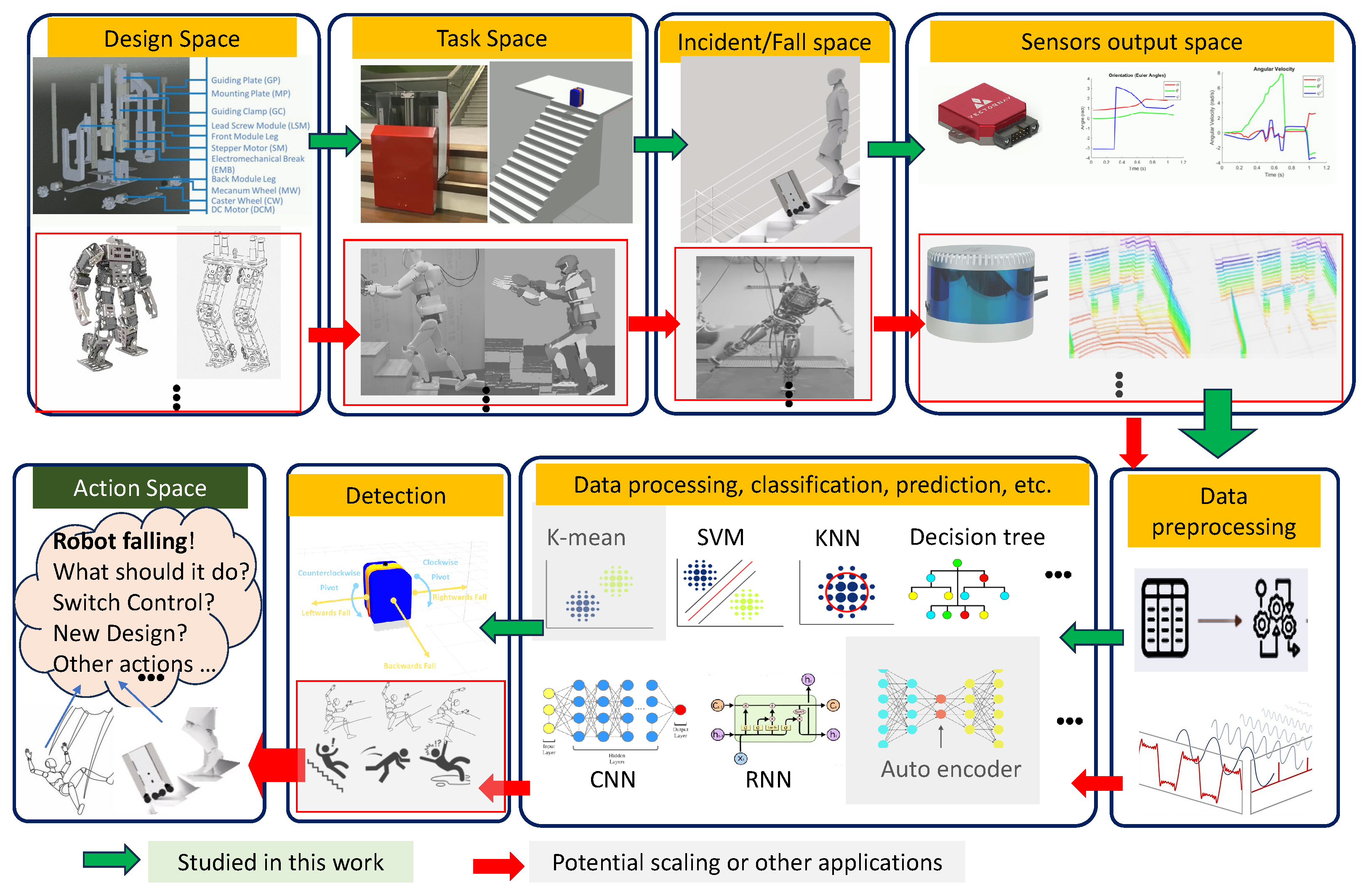
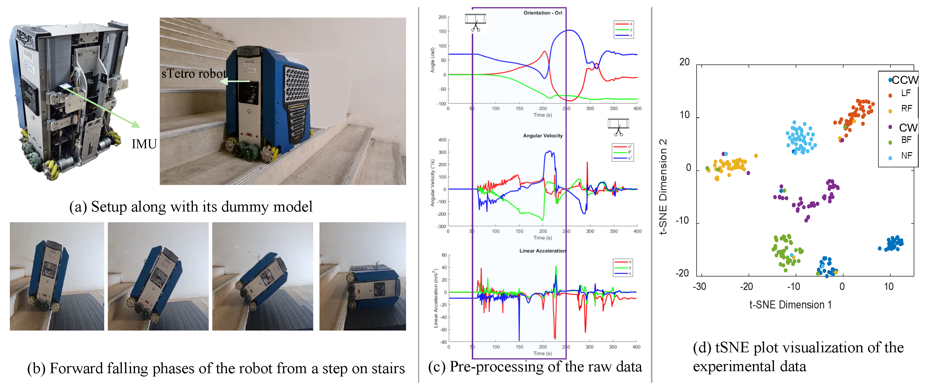
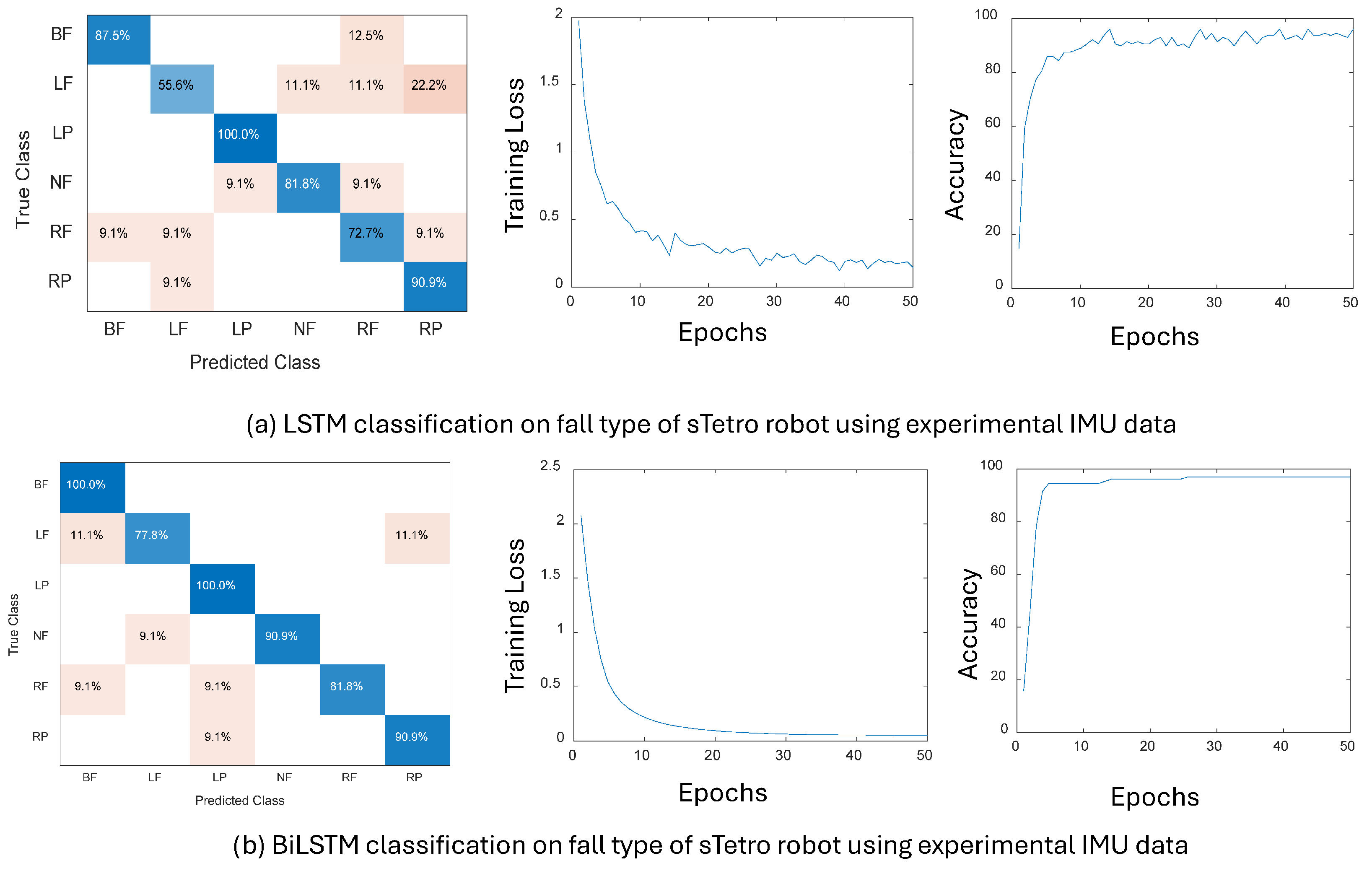
Table 1.
General advantages and disadvantages of different methods from the literature. Note that the referenced studies are often limited to humans or bipedal robots. This highlights a significant gap in research regarding fall detection for robots deployed in diverse conditions.
Table 1.
General advantages and disadvantages of different methods from the literature. Note that the referenced studies are often limited to humans or bipedal robots. This highlights a significant gap in research regarding fall detection for robots deployed in diverse conditions.
| Method | Advantages | Limitations |
|---|---|---|
| Conventional/Statistical methods [20,21,22,23] | Fast, easy to use, interpretable (linear) | Limited to low dimensions, not ideal for large datasets, doesn’t consider interactions between variables |
| Learning/classification methods [24,25,26,27,28,29,30,31] | Fast, handles missing data, accurate prediction, interpretable (sometimes) | Needs some expertise, can be computationally expensive |
| Deep Learning [32,33,34,35,36,37,38,39,40,41,42,43,44,45] | Effective, real-time processing (trained), handles large data and non-linearity | Slow to train, not always interpretable, generally requires large datasets |
Table 2.
Machine learning classification approaches.
| Approaches | Description |
|---|---|
| Naïve Bayes |
|
| KNN (k-Nearest Neighbors) |
|
| Decision Tree |
|
| SVM (Support Vector Machine) |
|
| Random Forest |
|
| Ensemble Technique |
|
Table 3.
Comparison of openloop and closedloop forecasting.
| Open Loop Forecasting | Closed Loop Forecasting |
|---|---|
| • Predicts the next time step in a sequence using only the input data. | Predicts subsequent time steps by using previous predictions as input. |
| • True values from the data source are used as input for subsequent time steps. | The model does not require true values for prediction. |
| • Useful when true values are available before making predictions. | Useful for forecasting multiple subsequent time steps. |
Table 4.
Range of values for different aspects of the applied force for each fall type. The origin for the position of force application is the center of the bottom-most surface of the central module.
Table 4.
Range of values for different aspects of the applied force for each fall type. The origin for the position of force application is the center of the bottom-most surface of the central module.
| Fall Types | Position [m] | Force [N] | ||||
|---|---|---|---|---|---|---|
| X | Y | Z | X | Y | Z | |
| BF | 0 | −0.1 to 0.1 | 0 to 0.45 | to | to 75 | to 75 |
| LF | to 0.1 | 0 | 0 to 0.45 | to 75 | 200 to 500 | to 75 |
| RF | to 0.1 | 0 | 0 to 0.45 | to 75 | to | to 75 |
| CCW | 0 | to | 0 to 0.45 | to | to 75 | to 75 |
| CW | 0 | 0.11 to 0.175 | 0 to 0.45 | to | to 75 | to 75 |
| NF | 0 | to 0.11 | 0 to 0.25 | to 0 | to 75 | to 75 |
Table 5.
The evaluation metrics for the different ML algorithms, indicating the Precision, Recall, and F1-scores.
Table 5.
The evaluation metrics for the different ML algorithms, indicating the Precision, Recall, and F1-scores.
| Class | Precision | Recall | F1 Score | ||||||
|---|---|---|---|---|---|---|---|---|---|
| NB | KNN | DT | NB | KNN | DT | NB | KNN | DT | |
| Class 1 (BF) | 0.62 | 0.9 | 0.83 | 0.43 | 0.85 | 0.82 | 0.51 | 0.87 | 0.82 |
| Class 2 (LF) | 0.46 | 0.98 | 0.97 | 0.87 | 0.98 | 0.97 | 0.61 | 0.98 | 0.97 |
| Class 3 (RF) | 0.9 | 0.99 | 0.98 | 0.84 | 0.98 | 0.97 | 0.87 | 0.98 | 0.97 |
| Class 4 (CCW) | 0.86 | 0.92 | 0.9 | 0.39 | 0.95 | 0.9 | 0.54 | 0.93 | 0.9 |
| Class 5 (CW) | 0.84 | 0.93 | 0.91 | 0.55 | 0.95 | 0.91 | 0.67 | 0.94 | 0.91 |
| Class 6 (NF) | 0.71 | 0.96 | 0.95 | 0.97 | 0.98 | 0.96 | 0.82 | 0.97 | 0.96 |
| Precision | Recall | F1 Score | |||||||
| SVM | RF | Enb | SVM | RF | Enb | SVM | RF | Enb | |
| Class 1 (BF) | 0.66 | 0.88 | 0.84 | 0.58 | 0.86 | 0.86 | 0.62 | 0.87 | 0.85 |
| Class 2 (LF) | 0.94 | 0.98 | 0.96 | 0.81 | 0.98 | 0.98 | 0.87 | 0.98 | 0.97 |
| Class 3 (RF) | 0.94 | 0.99 | 0.98 | 0.82 | 0.98 | 0.97 | 0.88 | 0.98 | 0.98 |
| Class 4 (CCW) | 0.8 | 0.93 | 0.94 | 0.69 | 0.93 | 0.9 | 0.74 | 0.93 | 0.92 |
| Class 5 (CW) | 0.8 | 0.93 | 0.93 | 0.7 | 0.94 | 0.92 | 0.74 | 0.93 | 0.92 |
| Class 6 (NF) | 0.58 | 0.96 | 0.95 | 0.95 | 0.98 | 0.98 | 0.72 | 0.97 | 0.97 |
Table 6.
Root mean squared error (RMSE) between the predicted and target readings using openloop forecasting with LSTM and BiLSTM models.
Table 6.
Root mean squared error (RMSE) between the predicted and target readings using openloop forecasting with LSTM and BiLSTM models.
| RMSE | w | x | y | z | ||||||
|---|---|---|---|---|---|---|---|---|---|---|
| BF Test 39 (LSTM) | 0.0113 | 0.0110 | 0.0137 | 0.0088 | 0.0472 | 0.0440 | 0.1013 | 0.0694 | 0.1179 | 0.0286 |
| All test Data (LSTM) | 0.0190 | 0.0202 | 0.0239 | 0.0164 | 0.0782 | 0.1029 | 0.0977 | 0.2053 | 0.2121 | 0.0899 |
| BF Test 39 (BiLSTM) | 0.0070 | 0.0056 | 0.0090 | 0.0058 | 0.0170 | 0.0097 | 0.0122 | 0.0597 | 0.0486 | 0.0278 |
| All test Data (BiLSTM) | 0.0102 | 0.0106 | 0.0128 | 0.0088 | 0.0257 | 0.0279 | 0.0269 | 0.0492 | 0.0432 | 0.0498 |
Table 7.
Root Mean Square Error (RMSE) for BiLSTM model with experimental data.
| Dataset | Roll | Pitch | Yaw | ||||||
|---|---|---|---|---|---|---|---|---|---|
| BF Test-10 | 0.0662 | 0.1140 | 0.1657 | 0.0738 | 0.0928 | 0.1420 | 0.1204 | 0.0618 | 0.0803 |
| All Test Data | 0.0896 | 0.1030 | 0.1058 | 0.0809 | 0.0833 | 0.1059 | 0.1463 | 0.1013 | 0.1034 |
Disclaimer/Publisher’s Note: The statements, opinions and data contained in all publications are solely those of the individual author(s) and contributor(s) and not of MDPI and/or the editor(s). MDPI and/or the editor(s) disclaim responsibility for any injury to people or property resulting from any ideas, methods, instructions or products referred to in the content. |
© 2024 by the authors. Licensee MDPI, Basel, Switzerland. This article is an open access article distributed under the terms and conditions of the Creative Commons Attribution (CC BY) license (https://creativecommons.org/licenses/by/4.0/).
Share and Cite
MDPI and ACS Style
Ong, J.H.; Hayat, A.A.; Gomez, B.F.; Elara, M.R.; Wood, K.L. Deep Learning Based Fall Recognition and Forecasting for Reconfigurable Stair-Accessing Service Robots. Mathematics 2024, 12, 1312. https://doi.org/10.3390/math12091312
AMA Style
Ong JH, Hayat AA, Gomez BF, Elara MR, Wood KL. Deep Learning Based Fall Recognition and Forecasting for Reconfigurable Stair-Accessing Service Robots. Mathematics. 2024; 12(9):1312. https://doi.org/10.3390/math12091312
Chicago/Turabian StyleOng, Jun Hua, Abdullah Aamir Hayat, Braulio Felix Gomez, Mohan Rajesh Elara, and Kristin Lee Wood. 2024. "Deep Learning Based Fall Recognition and Forecasting for Reconfigurable Stair-Accessing Service Robots" Mathematics 12, no. 9: 1312. https://doi.org/10.3390/math12091312
Note that from the first issue of 2016, this journal uses article numbers instead of page numbers. See further details here.