
Meshless Generalized Finite Difference Method Based on Nonlocal Differential Operators for Numerical Simulation of Elastostatics

1
School of Civil Engineering Architecture and the Environment, Hubei University of Technology, Wuhan 430068, China
2
State Key Laboratory of Geomechanics and Geotechnical Engineering, Institute of Rock and Soil Mechanics, Chinese Academy of Sciences, Wuhan 430071, China
3
Beijing Municipal Construction Group Co., Ltd., Beijing 100048, China
*
Author to whom correspondence should be addressed.
Mathematics 2024, 12(9), 1316; https://doi.org/10.3390/math12091316
Submission received: 24 March 2024
/
Revised: 23 April 2024
/
Accepted: 23 April 2024
/
Published: 25 April 2024
(This article belongs to the Special Issue Recent Advances in Numerical Methods for Scientific and Engineering Applications, 2nd Edition)
Abstract
:This study proposes an innovative meshless approach that merges the peridynamic differential operator (PDDO) with the generalized finite difference method (GFDM). Based on the PDDO theory, this method introduces a new nonlocal differential operator that aims to reduce the pre-assumption required for the PDDO method and simplify the calculation process. By discretizing through the particle approximation method, this technique proficiently preserves the PDDO’s nonlocal features, enhancing the numerical simulation’s flexibility and usability. Through the numerical simulation of classical elastic static problems, this article focuses on the evaluation of the calculation accuracy, calculation efficiency, robustness, and convergence of the method. This method is significantly stronger than the finite element method in many performance indicators. In fact, this study demonstrates the practicability and superiority of the proposed method in the field of elastic statics and provides a new approach to more complex problems.
1. Introduction
The numerical analysis of elastic statics plays a vital role in civil and mechanical engineering. Engineers can use the knowledge of elastic statics to predict the stress, strain, and displacement of structural members through numerical simulation before actual construction to evaluate the feasibility and safety of a project [1].
The finite element method (FEM) [2,3,4,5] is widely used in numerical analysis. However, when faced with problems involving large deformations and high-speed impacts, the grids may deform, leading to non-convergence. At the same time, when dealing with some complex problems, the computational cost of the FEM is usually higher compared to that of mesh-free methods [6]. The boundary element method (BEM) [7,8,9,10] focuses more on the processing and analysis of the boundary, reducing the discretization requirements of the internal points and improving the computational efficiency. The disadvantage is its limited ability to deal with nonlinear problems and the high computational cost of finding the internal solution. As one of the most common meshless methods, smoothed particle hydrodynamics (SPH) [11,12] has great advantages in dealing with complex geometric boundaries and large deformation problems. However, special treatment is usually required for boundary conditions, such as the arrangement of virtual particles [13]. Although this approach improves the accuracy and stability of the method, it significantly increases its computational cost. The Petrov–Galerkin method [14] also faces similar problems to those of the SPH method.
Based on the limitations of the aforementioned numerical simulation methods, this study introduces a new type of mesh-free method. This method refers to the theoretical basis of the two advanced calculation methods of the peridynamic differential operator (PDDO) and generalized finite difference method (GFDM) and combines their advantages. The primary objective of this study is to integrate the concept of Taylor expansion and the formulation of nonlocal integrals within the PDDO framework, leveraging the particle approximation method [15] frequently employed in SPH methods for discretizing these integrals. Subsequently, we aim to compute the necessary differential operators formulated through a weighted summation approach. Using differential operators to obtain the required partial derivatives, this step is crucial for the entire numerical simulation process because the accuracy of the differential operator directly determines the accuracy and reliability of the problem solving. By substituting these exact partial derivatives into the discrete equations constructed using the GFDM and solving the discrete equations, we can obtain physical quantities such as displacement and stress.
Peridynamics (PD) is a theory proposed by Silling et al. [16,17,18] to simulate the phenomenon of continuum mechanics. Unlike the traditional continuum mechanics method, PD describes the relationship between materials through the long-range interaction between material points, thus overcoming the difficulties in dealing with material fracture. Therefore, it has great advantages in dealing with cracks and fracture phenomena occurring inside the material. The peridynamic differential operator is a meshless method based on the nonlocal idea of PD proposed by Madenci [19,20] in 2016. Using the characteristics of Taylor series expansion and PD function, this method transforms the local differential into a widely applicable nonlocal integral form, realizes the numerical differential, and effectively avoids the discontinuity or singularity problems that may occur in the simulation process. The PDDO provides a nonlocal integral framework for this study, which makes approximations of the derivatives of physical quantities possible using the integral form without direct differentiation. When dealing with discontinuous problems, traditional differential methods encounter situations where the entire solution domain is not continuously derivable. In contrast, using the integral form to approximate the derivative is less susceptible to local discontinuities and can handle such discontinuities more precisely. Compared to the differential method, the integral form technique is more stable. This method has been widely used to simulate crack propagation [21], coupled stress [22], heat conduction [23], and other phenomena.
The generalized finite difference method, first proposed by Liszka [24] in 1980, is a meshless method with local control domain characteristics. It realizes the numerical solution of partial differential equations with the difference approximations of nodes in local regions. Since the GFDM is a meshless method that can arrange irregular nodes, it has unique advantages in dealing with problems with complex geometric boundaries. Many researchers have improved and perfected the GFDM through in-depth research over time [25,26,27], making its theoretical basis more mature and its application scope more extensive. The research of Hidayat [28] further demonstrates the effectiveness of the GFDM in solving two-dimensional elastic static problems. The GFDM is also widely used in the solution of partial differential equations [29] and the analysis of complex problems such as geotechnical engineering [30,31]. In these applications, the GFDM shows its unique advantages in dealing with irregular boundaries, multi-physics coupling, and nonlinear problems, thus playing a vital role in scientific research and engineering practice.
To evaluate the accuracy and efficiency of the method proposed in this article, we selected three classical examples for numerical simulation. In addition, the robustness and convergence of this method are discussed by changing the corresponding physical parameters [32]. Through the study of the above characteristics, the superiority of this method and its potential in simulating more complex problems are further illustrated.
2. Theoretical Knowledge
2.1. Deriving Partial Derivatives Using Nonlocal Differential Operators
In this section, the newly proposed nonlocal differential operator presented in this article is used to solve for partial derivatives. It mainly introduces how to use the Taylor series expansion and nonlocal properties of the PDDO, utilize the particle approximation method to discretize the corresponding differential operators, and incorporate the constructed partial derivatives into the GFDM of elastic constitutive relations to obtain variables such as displacement and stress.
Consider a field , where node serves as the point source, as illustrated in Figure 1. The influence range is determined by the internal nodes within the vicinity of . In this context, represents the smoothing length, and is the kernel coefficient. The distance between these points can be defined as with . In meshless methods, the distances between these nodes and the size of the support domain are usually considered infinitesimal.
For a two-dimensional problem, where , the field function () = is expanded using a second-order Taylor series:
where and are 0, 1, or 2 and represents the higher-order remainder term.
Taking the second-order Taylor expansion at a point within the influence domain of as an example,
we define the following:
Then, Equation (2) can be simplified to:
Ignoring the higher-order terms, we apply weighted integration to both sides of Equation (6):
where in a two-dimensional problem refers to the area of the influence domain of the point source and represents the weight function between the point source and a point within the computational domain. In the SPH method, this weight function can typically be a quintic spline kernel function, cubic spline kernel function, or Gaussian kernel function [15], with the quintic spline kernel function being presented as follows:
where in one-, two-, or three-dimensional spaces is 1/120, 7/478π, or 3/359π, respectively.
If we perform a second-order Taylor expansion for all particles within the entire computational domain with particle as the point source (assuming such points) and ignore the higher-order terms we can obtain a system of equations with as the unknown variable:
Inverting Equation (10) yields:
where:
In the process of converting integration into summation for discretization, the idea of the particle approximation method from the SPH method is referenced:
where and represent the mass and density, respectively, of a point within the computational domain with as the point source.
Combining Equations (11), (15), and (16) yields:
where represents:
From Equation (17), the numerical differentiation operator with as the point source can be obtained:
2.2. Elastic Constitutive of the Generalized Finite Difference Method
The governing equations for the elastic statics of a two-dimensional stress field, considering a constitutive model, where , , and represent the computational domain, displacement boundary, and traction boundary respectively, can be expressed as:
where is the stress tensor, represents the known components of body force, and , respectively, denote the cosine of the exterior normal and known components of traction on the boundary , represents the displacement components, and represents the known displacement components on the boundary , where and
Taking a two-dimensional plane stress problem as an example, Equations (20)–(22) can be expressed in terms of displacement components:
where is the elastic modulus, represents the Poisson’s ratio, and and are defined as:
The fundamental goal of the GFDM is to approximate partial derivatives at each node using the function values of surrounding nodes. This approximation is achieved by solving for weighted coefficients, making the partial derivatives at a specific node approximate to a linear combination of the function values of the surrounding nodes. The main formula can be expressed as:
By combining Equations (19), (23), and (28), we can obtain:
where denotes the row vector from the th row of the numerical differentiation operator based within the computational domain, with , acting as the point source. In this study, the penalty function method is used to deal with the given displacement and stress boundary conditions. Assuming that a point is a node with a given boundary condition on the boundary, the displacement and stress boundaries are:
where e is an extremely large penalty coefficient. If the boundary node has given displacements and stress boundary components, adding the boundary conditions determined by Equations (30)–(33) to the corresponding rows of Equation (29) yields:
The coefficient matrix is composed of the control equations for all nodes within the computational domain, together with the boundary equations for the boundary points, multiplied by the penalty coefficients e.
Inverting the system of equations enables the acquisition of the displacement components for each node:
3. Numerical Simulation
In this section, the effectiveness and applicability of the proposed method are verified with numerical simulation, and key characteristics, such as accuracy, computational efficiency, robustness, and convergence, are compared. To accurately evaluate the performance of this method, this study uses two indicators: normalized root mean square error and absolute error.
where and represent the normalized root mean square errors of displacement and stress, respectively. and are the numerical solutions for displacement and stress, respectively, and are the analytical solutions for displacement and stress, respectively. denotes the numerical solution obtained using this method, and represents the analytical solution.
Of note, the numerical simulation results of the following examples are based on the MATLAB R2023b program and were completed using an AMD Ryzen 9 5900HX eight-core processor.
3.1. Cantilever Beam Subjected to Shear Force
In the first example, as illustrated in Figure 2, we consider a cantilever beam with length , width , Poisson’s ratio , and elastic modulus In addition, represents the moment of inertia, and for a rectangular beam of unit thickness, the moment of inertia . The integral of the distributed force, which is the shear load , is also considered. For plane stress problems, the analytical solutions [33] for displacement and strain are:
3.1.1. Error Analysis
To evaluate the precision and computational speed of this method following adjustments to specific parameters, this study arranged nodes in configurations of 5 × 17, 7 × 25, 13 × 49, 16 × 61, 21 × 81, and 31 × 121 along the x- and y-axes, adopting a third-order Taylor expansion. This study employed computational approaches based on the cubic spline kernel function, quintic spline kernel function, and Gaussian kernel function, comparing these with the computational outcomes derived from the FEM.
As shown in Table 1, compared to the FEM, the proposed method demonstrates higher accuracy and computational efficiency, where the execution time was obtained using MATLAB’s tic-toc function. Moreover, it achieves greater accuracy with the quintic spline and cubic spline kernel functions. Although the scheme using the Gaussian kernel function has slightly lower accuracy, its computation time is marginally less than that of the aforementioned schemes. From a computational cost perspective, this method requires only a small number of nodes to achieve high-accuracy results. Because of the method’s provision of highly accurate differential operators, high-precision spatial derivatives are obtained in the process of deriving stress from displacement, resulting in stress errors very close to displacement errors.
Figure 3 and Figure 4 illustrate a comparison between the numerical solution for the stress components of a cantilever beam obtained with this method and the analytical solution, employing the quintic spline kernel function, with a node quantity N = 5 × 17 = 85 and a Taylor expansion order K = 3. The numerical solution closely matches the analytical solution in both magnitude and distribution.
3.1.2. Robustness Analysis
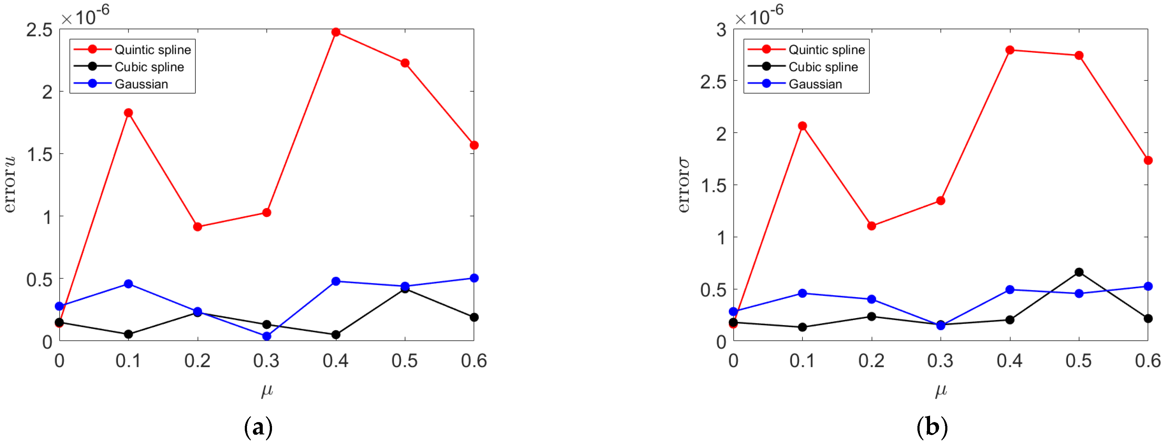
To further investigate the ability of the proposed method to maintain its predictive accuracy and operational stability when facing various challenges, changes, or external disturbances, this study introduces the perturbation coefficient μ, which is defined using the following formula:
where represents the coordinates of internal nodes (excluding boundary nodes), is the smoothing length, is a random displacement within the smoothing length, satisfying the condition , and represents the updated node coordinates. In this way, as the perturbation coefficient μ increases, the initial arrangement of nodes becomes more chaotic. Figure 5a–c show the initial arrangement of nodes when μ is set to 0, 0.3, and 0.6, respectively. As the perturbation coefficient μ increases, the initial distribution of nodes becomes more chaotic.
Figure 6 illustrates the relationship between the perturbation coefficient μ and displacement and stress errors. The displacement and stress errors associated with the quintic spline kernel function are most significantly impacted by the increase in node disorder. However, the range of error variation remains within an order of magnitude. In contrast, the impact on accuracy using the other two methods is very limited and almost negligible despite the increase in the perturbation coefficient μ.
From the analysis of the error variation relationship between the perturbation coefficient μ and each kernel function, the corresponding conclusion can be drawn: although the quintic spline kernel function is more sensitive to the influence of the disturbance amplitude, the method still has good robustness as a whole.
3.1.3. Convergence Analysis
This section explores the convergence of the methods used in this study, especially the specific effects of the number of nodes and the Taylor expansion order on the accuracy.
In this study, the initial node layout schemes of 85, 175, 637, 976, and 1701 nodes were adopted. Figure 7 shows a decreasing trend in the displacement error and stress error with the increase in the number of nodes N, and a monotonous negative correlation exists between the two, indicating the method has good convergence and stability. At the same time, as the Taylor expansion order increases from K = 3 to K = 4, the displacement error and stress error obtained with the method of different kernel functions decrease, which also confirms that the method has good convergence.
3.2. Analysis of the Surrounding Rock Compression for a Circular Tunnel
As shown in Figure 8, a circular tunnel surrounded by rock is subjected to uniform external pressure. The inner radius , the outer radius , with an elastic modulus and a Poisson’s ratio of . The external pressure and the internal pressure . The analytical solutions [34] for displacement and stress are as follows:
3.2.1. Error Analysis
In this section, nodes were arranged tangentially and radially in configurations of 11 × 19, 19 × 29, 25 × 39, and 33 × 49. Figure 9 shows the comparison between the numerical solution and the analytical solution when the Taylor expansion order K = 4, using the quintic kernel function. According to Table 2, the cubic spline kernel function, quintic spline function, and Gaussian kernel function all exhibit high accuracy, with displacement and stress errors on the order of 10−3. Although the accuracy is slightly lower than the FEM, the computation time is significantly less than that of the FEM. Additionally, compared to the FEM, the difference between displacement and stress errors in this method is minimal. This is attributed to the method’s differential operator providing high-accuracy partial derivatives, resulting in smaller errors in the stress components derived from displacement components.
3.2.2. Robustness Analysis
This section utilizes both regular and irregular nodes (with a perturbation coefficient μ 0.2), as shown in Figure 10. Given the symmetry of this example, the robustness analysis in this case only requires comparing the displacement and stress components along the x-axis. Figure 11 and Figure 12 display the numerical solutions for displacement and stress under regular and irregular initial node distributions, respectively, along with the absolute errors compared to the analytical solutions.
As shown in Figure 11, when employing a regular arrangement of initial nodes, the maximum absolute error of displacement along the x-axis only reaches the level of 2 × 10⁻⁵, and it is confined to a small portion within the inner radius range. When using an irregular node arrangement, the displacement along the x-axis increases progressively, with a maximum of 8 × 10⁻⁵. Although this is an increase compared to the regular node distribution, it still significantly differs from numerical solutions at the 10−3 level. Figure 12 shows that although the area of the absolute error of the stress becomes larger when the nodes are arranged irregularly, the maximum value decreases. From the perspective of displacement and stress errors, in this example, this method shows a low sensitivity to the confusion of the initial node arrangement.
3.2.3. Convergence Analysis
This section analyzes the displacement and stress errors when using different kernel functions and orders of Taylor expansions with node quantities of 209, 551, 975, and 1617. As shown in Figure 13, with an increase in the number of nodes, the precision of the calculations improves. In conjunction with Example 1 in Figure 7, the methods employing the three types of kernel functions all exhibit convergence, and the rate of decrease in errors gradually slows as the number of nodes increases. Additionally, using a higher order of Taylor expansion significantly enhances the accuracy of the method, bringing it closer to the analytical solution.
3.3. Homogeneous Slope Subjected to Self-Weight
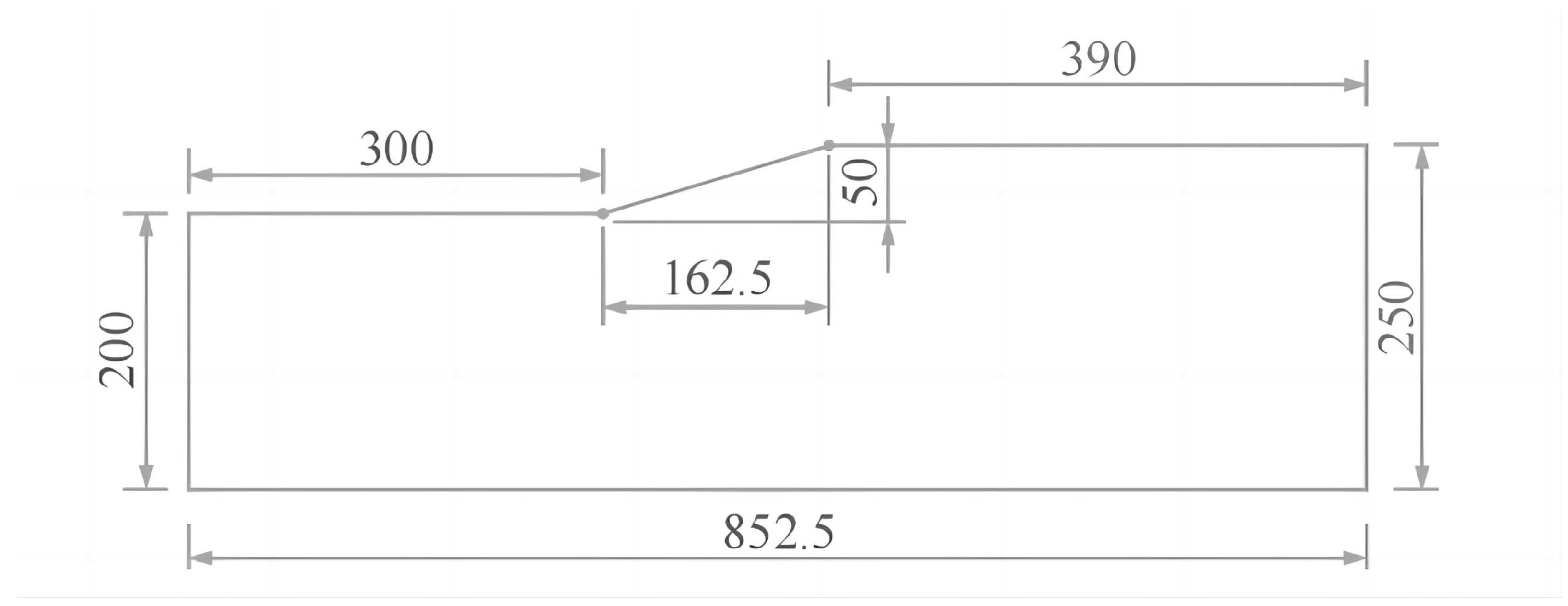
Next, we consider a homogeneous slope solely subjected to self-weight [35], and Figure 14 displays its geometric model. The material properties are as follows: elastic modulus E = 80 MPa, unit weight γ = 19.62 kN/m3, and Poisson’s ratio v = 0.43. The model’s base is fully fixed, with normal constraints applied to its sides.
This research deployed the FEM to set up a dense network of nodes and elements (86,372 nodes and 85,650 quadrilateral elements) to derive a reliable reference solution for comparison with the results from the GFDM.
Figure 15 shows the computational outcomes of this approach versus the FEM, while Table 3 presents the maximum values for displacement and stress components from this method alongside the reference solution. Figure 15 and Table 3 demonstrate that the magnitude and distribution of results from this method closely match the reference solution obtained with the FEM.
4. Conclusions
This article introduces a meshless method that leverages the strengths of the PDDO and GFDM. This approach retains the nonlocal characteristics of the PDDO while reducing many preliminary assumptions. Unlike traditional meshless methods, it does not require special treatment of boundary conditions, making it easier to implement and more computationally efficient. Numerical simulations of several classic examples compared with traditional numerical methods (FEM) verify its superior performance in terms of accuracy, efficiency, robustness, and convergence. In particular, it demonstrates high adaptability and robustness in scenarios of irregular node arrangements, increased perturbation coefficients, and more nodes, confirming its potential in solving complex engineering problems.
In conclusion, the meshless numerical simulation method combining the PDDO and GFDM proposed in this study provides a new solution in the field of numerical analysis of elastic statics. Future work will focus on further expanding the application scope of this method, including exploring its effectiveness in dealing with more complex multi-physics problems and improving numerical algorithms to achieve higher accuracy and computational efficiency.
Author Contributions
Conceptualization, C.L.; methodology, C.L.; software, C.L. and Y.Z.; validation, C.L.; formal analysis, C.L. and Y.Z.; resources, C.L. and Y.Z.; data curation, C.L. and Y.Z.; writing—original draft preparation, Y.Z.; writing—review and editing, Y.Z.; visualization, Y.Z. and Z.W.; supervision, X.Z.; project administration, X.Z. and C.L. All authors have read and agreed to the published version of the manuscript.
Funding
This research received no funding.
Data Availability Statement
The data are included in this article and can be found within the figures and tables.
Acknowledgments
The authors express their gratitude for the constructive comments provided by the anonymous reviewers.
Conflicts of Interest
The third author, Zhifen Wang, is employed by Beijing Municipal Construction Group Co., Ltd. The other authors declare that this study was conducted in the absence of any commercial or financial relationships that could be construed as a potential conflict of interest.
References
- Ericksen, J.L. Special topics in elastostatics. Adv. Appl. Mech. 1977, 17, 189–244. [Google Scholar]
- Deeks, A.J.; Wolf, J. A virtual work derivation of the scaled boundary finite-element method for elastostatics. Comput. Mech. 2002, 28, 489–504. [Google Scholar] [CrossRef]
- Kamiński, M. Generalized perturbation-based stochastic finite element method in elastostatics. Comput. Struct. 2007, 85, 586–594. [Google Scholar] [CrossRef]
- Vadlamani, S.; Arun, C. A stochastic B-spline wavelet on the interval finite element method for beams. Comput. Struct. 2020, 233, 106246. [Google Scholar] [CrossRef]
- Mohammad, M.; Trounev, A.; Cattani, C. Stress state and waves in the lithospheric plate simulation: A 3rd generation AI architecture. Results Phys. 2023, 53, 106938. [Google Scholar] [CrossRef]
- Zhang, X.; Zhang, P.; Zhang, L. A simple technique to improve computational efficiency of meshless methods. Procedia Eng. 2012, 31, 1102–1107. [Google Scholar] [CrossRef]
- Wang, Q.; Zhou, W.; Cheng, Y.; Ma, G.; Chang, X.; Huang, Q. The boundary element method with a fast multipole accelerated integration technique for 3D elastostatic problems with arbitrary body forces. J. Sci. Comput. 2017, 71, 1238–1264. [Google Scholar] [CrossRef]
- Hamzehei Javaran, S.; Shojaee, S. The solution of elastostatic and dynamic problems using the boundary element method based on spherical Hankel element framework. Int. J. Numer. Meth. Eng. 2017, 112, 2067–2086. [Google Scholar] [CrossRef]
- Bin, H.; Zhongrong, N.; Cong, L.; Zongjun, H. A fast multipole boundary element method based on higher order elements for analyzing 2-D elastostatic problems. Eng. Anal. Bound. Elem. 2021, 130, 417–428. [Google Scholar] [CrossRef]
- Vu, D.; Steinmann, P. A 2-D coupled BEM–FEM simulation of electro-elastostatics at large strain. Comput. Methods. Appl. Mech. Eng. 2010, 199, 1124–1133. [Google Scholar] [CrossRef]
- Gray, J.P.; Monaghan, J.J.; Swift, R. SPH elastic dynamics. Comput. Methods Appl. Mech. Eng. 2001, 190, 6641–6662. [Google Scholar] [CrossRef]
- Shutov, A.; Klyuchantsev, V. On the application of SPH to solid mechanics. J. Phys. Conf. Ser. 2019, 1268, 012077. [Google Scholar] [CrossRef]
- El-Gammal, T.; Khalil, E.; Haridy, H.; Abo-Serie, E. Influence of smoothing length and virtual particles on SPH accuracy. Int. J. Mater. Mech. Manuf. 2013, 1, 166–170. [Google Scholar] [CrossRef]
- Atluri, S.; Zhu, T.-L. The meshless local Petrov-Galerkin (MLPG) approach for solving problems in elasto-statics. Comput. Mech. 2000, 25, 169–179. [Google Scholar] [CrossRef]
- Liu, M.; Liu, G. Smoothed particle hydrodynamics (SPH): An overview and recent developments. Arch. Comput. Methods Eng. 2010, 17, 25–76. [Google Scholar] [CrossRef]
- Silling, S.A. Reformulation of elasticity theory for discontinuities and long-range forces. J. Mech. Phys. Solids. 2000, 48, 175–209. [Google Scholar] [CrossRef]
- Silling, S.A.; Lehoucq, R.B. Peridynamic theory of solid mechanics. Adv. Appl. Mech. 2010, 44, 73–168. [Google Scholar]
- Silling, S.A.; Askari, E. A meshfree method based on the peridynamic model of solid mechanics. Comput. Struct. 2005, 83, 1526–1535. [Google Scholar] [CrossRef]
- Madenci, E.; Barut, A.; Futch, M. Peridynamic differential operator and its applications. Comput. Methods. Appl. Mech. Eng. 2016, 304, 408–451. [Google Scholar] [CrossRef]
- Madenci, E.; Barut, A.; Dorduncu, M. Peridynamic Differential Operator for Numerical Analysis; Springer: Berlin/Heidelberg, Germany, 2019; Volume 10. [Google Scholar]
- Wan, J.; Yang, D.; Chu, X.; Qu, W. A micropolar peridynamic differential operator and simulation of crack propagation. Eng. Fract. Mech. 2022, 269, 108532. [Google Scholar] [CrossRef]
- Lei, J.; Sun, Y.; Wang, L. Static and dynamic analysis of couple-stress elastic structures by using peridynamic differential operator. Eng. Anal. Bound. Elem. 2023, 156, 20–33. [Google Scholar] [CrossRef]
- Zhou, B.; Li, Z.; Xu, Y.; Huang, D. Analysis of nonlinear heat conduction problems with temperature-dependent conductivity using peridynamic differential operator. Int. J. Appl. Mech. 2022, 14, 2250047. [Google Scholar] [CrossRef]
- Liszka, T.; Orkisz, J. The finite difference method at arbitrary irregular grids and its application in applied mechanics. Comput. Struct. 1980, 11, 83–95. [Google Scholar] [CrossRef]
- Benito, J.; Urena, F.; Gavete, L. Influence of several factors in the generalized finite difference method. Appl. Math. Model. 2001, 25, 1039–1053. [Google Scholar] [CrossRef]
- Gavete, L.; Gavete, M.; Benito, J. Improvements of generalized finite difference method and comparison with other meshless method. Appl. Math. Model. 2003, 27, 831–847. [Google Scholar] [CrossRef]
- Zheng, Z.; Li, X. Theoretical analysis of the generalized finite difference method. Comput. Math. Appl. 2022, 120, 1–14. [Google Scholar] [CrossRef]
- Hidayat, M.I.P.; Fajarin, R. A meshless generalized finite difference method for 2D elasticity problems. Eng. Anal. Bound. Elem. 2020, 117, 89–103. [Google Scholar] [CrossRef]
- Suchde, P.; Kuhnert, J. A meshfree generalized finite difference method for surface PDEs. Comput. Math. Appl. 2019, 78, 2789–2805. [Google Scholar] [CrossRef]
- Benito, J.; Ureña, F.; Salete, E.; Muelas, A.; Gavete, L.; Galindo, R. Wave propagation in soils problems using the Generalized Finite Difference Method. Soil. Dyn. Earthq. Eng. 2015, 79, 190–198. [Google Scholar] [CrossRef]
- Liu, Y.; Rao, X.; Zhao, H.; Zhan, W.; Xu, Y.; Liu, Y. Generalized finite difference method based meshless analysis for coupled two-phase porous flow and geomechanics. Eng. Anal. Bound. Elem. 2023, 146, 184–203. [Google Scholar] [CrossRef]
- Li, H.; Mulay, S.S. Meshless Methods and Their Numerical Properties; CRC Press: Boca Raton, FL, USA, 2013. [Google Scholar]
- Wang, J.; Liu, G. A point interpolation meshless method based on radial basis functions. Int. J. Numer. Meth. Eng. 2002, 54, 1623–1648. [Google Scholar] [CrossRef]
- Liu, G.; Zhang, J.; Li, H.; Lam, K.; Kee, B.B. Radial point interpolation based finite difference method for mechanics problems. Int. J. Numer. Meth. Eng. 2006, 68, 728–754. [Google Scholar] [CrossRef]
- Zheng, H.; Liu, D.; Li, C.G. Slope stability analysis based on elasto-plastic finite element method. Int. J. Numer. Meth. Eng. 2005, 64, 1871–1888. [Google Scholar] [CrossRef]
Figure 1.
Point source and the internal points within its support domain.

Figure 2.
Cantilever beam subjected to shear force.

Figure 3.
Example 1: Comparison of analytical and numerical solutions for deformation of 85 nodes.

Figure 4.
Relative errors of stress components: (a) comparison of the analytical and numerical solutions for normal stress in the x-direction and (b) comparison of the analytical and numerical solutions for shear stress.
Figure 4.
Relative errors of stress components: (a) comparison of the analytical and numerical solutions for normal stress in the x-direction and (b) comparison of the analytical and numerical solutions for shear stress.

Figure 5.
Initial arrangement of nodes for different perturbation coefficients μ of (a) 0, (b) 0.3, and (c) 0.6.
Figure 5.
Initial arrangement of nodes for different perturbation coefficients μ of (a) 0, (b) 0.3, and (c) 0.6.

Figure 6.
(a) Relationship between displacement and perturbation coefficient; (b) relationship between stress and perturbation coefficient.
Figure 6.
(a) Relationship between displacement and perturbation coefficient; (b) relationship between stress and perturbation coefficient.

Figure 7.
(a) Relationship between node number and displacement error; (b) relationship between node number and stress error.
Figure 7.
(a) Relationship between node number and displacement error; (b) relationship between node number and stress error.

Figure 8.
Circular tunnel subjected to external rock pressure.

Figure 9.
Example 2: Comparison of analytical and numerical solutions for deformation of 85 nodes.

Figure 10.
Initial node arrangements for Example 2: (a) regular (μ = 0) and (b) irregular (μ = 0.2).
Figure 10.
Initial node arrangements for Example 2: (a) regular (μ = 0) and (b) irregular (μ = 0.2).

Figure 11.
Displacement in Example 2: (a) magnitude of displacement components and absolute errors with regular initial node arrangement; (b) magnitude of displacement components and absolute errors with irregular initial node arrangement.
Figure 11.
Displacement in Example 2: (a) magnitude of displacement components and absolute errors with regular initial node arrangement; (b) magnitude of displacement components and absolute errors with irregular initial node arrangement.

Figure 12.
Stress in Example 2: (a) magnitude of stress components and absolute errors with regular initial node arrangement; (b) magnitude of stress components and absolute errors with irregular initial node arrangement.
Figure 12.
Stress in Example 2: (a) magnitude of stress components and absolute errors with regular initial node arrangement; (b) magnitude of stress components and absolute errors with irregular initial node arrangement.

Figure 13.
(a) Relationship between displacement error and node number under different kernel functions and Taylor expansion orders; (b) relationship between stress error and node number under different kernel functions and Taylor expansion orders.
Figure 13.
(a) Relationship between displacement error and node number under different kernel functions and Taylor expansion orders; (b) relationship between stress error and node number under different kernel functions and Taylor expansion orders.

Figure 14.
Homogeneous slope subjected to self-weight.

Figure 15.
(a) Numerical solutions for displacement and stress components obtained using the GFDM; (b) reference solutions for displacement and stress components obtained with the FEM.
Figure 15.
(a) Numerical solutions for displacement and stress components obtained using the GFDM; (b) reference solutions for displacement and stress components obtained with the FEM.


Table 1.
Example 1: Comparison of displacement and stress errors and computational efficiency of each method at different numbers of nodes.
Table 1.
Example 1: Comparison of displacement and stress errors and computational efficiency of each method at different numbers of nodes.
| Method | N = 85 | N = 175 | N = 637 | N = 976 | N = 1701 | N = 3751 | |
|---|---|---|---|---|---|---|---|
| Cubic spline | 1.1559 × 10⁻⁶ | 1.0396 × 10⁻⁶ | 7.4807 × 10⁻⁷ | 6.7813 × 10⁻⁷ | 5.5154 × 10⁻⁷ | 4.1265 × 10⁻⁷ | |
| 1.3159 × 10⁻⁶ | 1.1633 × 10⁻⁶ | 8.9742 × 10⁻⁷ | 7.5859 × 10⁻⁷ | 6.6085 × 10⁻⁷ | 5.4193 × 10⁻⁷ | ||
| Execution time (s) | 0.0221 | 0.0436 | 0.1532 | 0.2605 | 0.6728 | 1.6735 | |
| Quintic spline | 1.1043 × 10⁻⁶ | 9.6119 × 10⁻⁷ | 7.0886 × 10⁻⁷ | 5.8304 × 10⁻⁷ | 4.8986 × 10⁻⁷ | 3.7597 × 10⁻⁷ | |
| 1.2215 × 10⁻⁶ | 1.1276 × 10⁻⁶ | 8.1298 × 10⁻⁷ | 6.8245 × 10⁻⁷ | 5.9064 × 10⁻⁷ | 4.8986 × 10⁻⁷ | ||
| Execution time (s) | 0.0223 | 0.0483 | 0.1656 | 0.2906 | 0.6842 | 1.6972 | |
| Gaussian | 1.8407 × 10⁻⁶ | 1.6557 × 10⁻⁶ | 1.3924 × 10⁻⁶ | 1.1752 × 10⁻⁶ | 1.0110 × 10⁻⁶ | 9.0412 × 10⁻⁷ | |
| 1.9360 × 10⁻⁶ | 1.7710 × 10⁻⁶ | 1.5148 × 10⁻⁶ | 1.2638 × 10⁻⁶ | 1.0894 × 10⁻⁶ | 1.0310 × 10⁻⁶ | ||
| Execution time (s) | 0.0234 | 0.0443 | 0.1352 | 0.2557 | 0.6335 | 1.6421 | |
| FEM | 1.5878 × 10⁻³ | 7.1529 × 10⁻⁴ | 1.8235 × 10⁻⁴ | 1.1561 × 10⁻⁴ | 6.3913 × 10⁻⁵ | 1.8732 × 10⁻⁵ | |
| 7.3210 × 10⁻² | 4.3649 × 10⁻² | 1.7055 × 10⁻² | 1.2465 × 10⁻² | 8.2747 × 10⁻³ | 2.4296 × 10⁻³ | ||
| Execution time (s) | 0.0740 | 0.1238 | 0.3882 | 0.7605 | 1.4390 | 3.1675 |
Table 2.
Example 2: Comparison of displacement and stress errors and computational efficiency of each method at different node numbers.
Table 2.
Example 2: Comparison of displacement and stress errors and computational efficiency of each method at different node numbers.
| Method | N = 209 | N = 551 | N = 975 | N = 1617 | |
|---|---|---|---|---|---|
| Cubic spline | 7.2163 × 10⁻³ | 5.7165 × 10⁻³ | 4.5403 × 10⁻³ | 3.4731 × 10⁻³ | |
| 8.4958 × 10⁻³ | 6.6441 × 10⁻³ | 5.3892 × 10⁻³ | 4.2186 × 10⁻³ | ||
| Execution time (s) | 0.0912 | 0.1732 | 0.3984 | 0.8547 | |
| Quintic spline | 6.1713 × 10⁻³ | 4.5487 × 10⁻³ | 3.1723 × 10⁻³ | 1.9475 × 10⁻³ | |
| 7.2931 × 10⁻³ | 5.5299 × 10⁻³ | 3.7452 × 10⁻³ | 2.4782 × 10⁻³ | ||
| Execution time (s) | 0.1031 | 0.1973 | 0.4134 | 0.8835 | |
| Gaussian | 9.9101 × 10⁻³ | 8.6321 × 10⁻³ | 7.3814 × 10⁻³ | 6.1756 × 10⁻³ | |
| 1. 0927 × 10−2 | 9.2074 × 10⁻³ | 7.6133 × 10⁻³ | 6.2943 × 10⁻³ | ||
| Execution time (s) | 0.1074 | 0.1867 | 0.4007 | 0.8379 | |
| FEM | 4.8610 × 10⁻⁴ | 2.5399 × 10⁻⁴ | 1.6901 × 10⁻⁴ | 1.1947 × 10⁻⁴ | |
| 8.0192 × 10⁻³ | 5.7098 × 10⁻³ | 4.4219 × 10⁻³ | 3.7964 × 10⁻³ | ||
| Execution time (s) | 0.3944 | 0.7821 | 1.6741 | 3.5971 |
Table 3.
Maximum values of displacement and stress components for the GFDM and FEM.
| Method | Max | |
|---|---|---|
| Ux (m) | GFDM | 0.425927 |
| FEM | 0.425957 | |
| Uy (m) | GFDM | 6.30321 |
| FEM | 6.30359 | |
| σx (Pa) | GFDM | 2.10600 × 10⁶ |
| FEM | 2.09875 × 10⁶ | |
| σy (Pa) | GFDM | 4.89859 × 10⁶ |
| FEM | 4.88162 × 10⁶ | |
| τxy (Pa) | GFDM | 2.07472 × 10⁵ |
| FEM | 2.07541 × 10⁵ |
Disclaimer/Publisher’s Note: The statements, opinions and data contained in all publications are solely those of the individual author(s) and contributor(s) and not of MDPI and/or the editor(s). MDPI and/or the editor(s) disclaim responsibility for any injury to people or property resulting from any ideas, methods, instructions or products referred to in the content. |
© 2024 by the authors. Licensee MDPI, Basel, Switzerland. This article is an open access article distributed under the terms and conditions of the Creative Commons Attribution (CC BY) license (https://creativecommons.org/licenses/by/4.0/).
Share and Cite
MDPI and ACS Style
Zhou, Y.; Li, C.; Zhuang, X.; Wang, Z. Meshless Generalized Finite Difference Method Based on Nonlocal Differential Operators for Numerical Simulation of Elastostatics. Mathematics 2024, 12, 1316. https://doi.org/10.3390/math12091316
AMA Style
Zhou Y, Li C, Zhuang X, Wang Z. Meshless Generalized Finite Difference Method Based on Nonlocal Differential Operators for Numerical Simulation of Elastostatics. Mathematics. 2024; 12(9):1316. https://doi.org/10.3390/math12091316
Chicago/Turabian StyleZhou, Yeying, Chunguang Li, Xinshan Zhuang, and Zhifen Wang. 2024. "Meshless Generalized Finite Difference Method Based on Nonlocal Differential Operators for Numerical Simulation of Elastostatics" Mathematics 12, no. 9: 1316. https://doi.org/10.3390/math12091316
Note that from the first issue of 2016, this journal uses article numbers instead of page numbers. See further details here.