HIV vs. the Immune System: A Differential Game

Abstract

A differential game is formulated in order to model the interaction between the immune system and the HIV virus. One player is represented by the immune system of a patient subject to a therapeutic treatment and the other player is the HIV virus. The aim of our study is to determine the optimal therapy that allows to prevent viral replication inside the body, so as to reduce the damage caused to the immune system, and allow greater survival and quality of life. We propose a model that considers all the most common classes of antiretroviral drugs taking into account different immune cells dynamics. We validate the model with numerical simulations, and determine optimal structured treatment interruption (STI) schedules for medications.

1. Introduction

The genetic code of the HIV virus consists of a ribonucleic acid, the RNA. HIV belongs to the retroviruses family, characterized by the presence of an enzyme, DNA-polymerase RNA-independent, capable of transcribing the genetic code RNA into DNA. This ability allows the virus to integrate its genome into the one of the cells it infects, so that the integrated virus would not be defeated nor by the immune response nor by drugs.

HIV has a marked tendency to mutate: mutations are errors that individual viral particles make in replicative cycles. Each error leads to the appearance of a virus, which is more or less analogous to the original one. Mutations are mostly “disadvantageous” for the viral species, as mutated viruses tend to disappear. Nevertheless some mutations are “beneficial” and allow mutated viruses to acquire drug resistance and immune response. One of the most effective mechanisms used by HIV to evade the immune response and treatment is, in fact, its aptitude to change.

The main HIV target cells are T lymphocytes of type CD4, fundamental in the adaptive response against a variety of pathogens and oncogenes.

The overall function of the immune system is to prevent or limit infections. An immune response is generally divided into innate and adaptive immunity. Innate immunity occurs immediately, when circulating innate cells recognize a problem. Adaptive immunity occurs later, as it relies on the coordination and expansion of specific adaptive immune cells.

In particular, CD4+ lymphocytes are very important cells in the immune system, in fact they recognize the various uninvited guests organism (viruses, bacteria, protozoa, fungi, worms and cancer cells) through biochemical messages, and they activate the areas of the immune system most suitable to counter their presence. A large number of CD4+ paralyzes the immune system, exposing the body to any risk of infection and cancer [1].

Actually, HIV can be suppressed by a combination of antiretroviral therapy (ART) consisting of three or more antiretroviral (ARV) drugs. In principle, ART cannot eradicate HIV infection from the “sanctuaries” (mainly lymph-nodes and lymphatic system); it controls viral replication within a body reducing viral burden, thus in turn it allows a functional improvement of an individual’s immune system that basically regains the capacity to fight off infections [2]. It has been proved that people with HIV, subject to ART therapy, can have a healthy and productive life, in fact after the advent of the ART therapy the mortality curve of HIV-infected patients started to decline.

On the other hand, the lack of a definitive eradication of viral reservoirs determines two important consequences: the anti-HIV treatment should be life-long; the longer the treatment, the more likely the development of drug-resistance. On this basis, an intense research activity has been developed in last decades, usefully enlarging the anti-HIV molecules repertoire. Actually there are more than 20 approved antiretroviral drugs, divided into 6 different pharmacological classes. Anti-retroviral drugs are broadly classified through the phase of the retrovirus life-cycle that they inhibit, as follows

• Nucleoside/Nucleotide Reverse Transcriptase Inhibitors (NRTI);
• Non-Nucleoside Reverse Transcriptase Inhibitors (NNRTI);
• Protease inhibitors (PI);
• Fusion Inhibitors (FI);
• Coreceptor Antagonists (CA);
• Integrase Inhibitors (II).

Typical combinations involve the conjunctive use of either two NRTIs and one NNRTI, or one PI (with or without Ritonavir) in combination with two NRTIs.

HAART (Highly active antiretroviral therapy) is an abbreviation for all protocols involving combinations of drugs, which are active against different molecular targets in the life cycle of HIV. These medications are administered in the form of the high concentration cocktails. This approach was born in 1995–1996 with the introduction of the second class of antiretroviral drugs: Protease inhibitor (PI), administered in combination with drugs of the first generation, or Reverse Transcriptase Inhibitors (NRTI and NNRTI: see zidovudine or AZT azidothymidine).

Among the benefits of treatment there is a decreased risk of progression to AIDS and a decreased risk of death. The adverse effects and the complexity of treatment regimens (due to the high number of pills and to dosing frequency) may reduce patient’s compliance [3].

A correct administration of antiretroviral drugs should be daily scheduled and uninterrupted; it requires care and precision, even in relation to meals and to subministration of other drugs. The omission of a few doses leads to a reduction of drug concentration in blood, therefore the residual level could become lower than the one necessary to inhibit the virus. Not only does this allow the resumption of viral replication, but it also facilitates the inexorable emergence of resistant virus. Resistant mutants tend to persist, making the drug ineffective, even if the intake of drugs is carried out according to the rhythms and the correct doses. A scarce adherence to the prescriptions and its consequent emergence of resistant mutants may cause failure of the treatment.

The therapy must prevent viral replication in the body, rather than the complete eradication of the infection, that remains chronic, so as to reduce the damage caused to the immune system and to allow greater survival and quality of life.

The study of HIV biological evolution and of its relationship with the immune system is used to determine a therapy policy that can defeat the viruses. Despite it seems counterintuitive, the aim is to determine a proper dosage of drugs, which defends against viruses only moderately and which may benefit both the host and the virus, i.e., without creating strong environmental pressures. A stable long-term coexistence can be reached, hopefully avoiding drug-resistance development.

Mathematical modeling of HIV infection has proven to be instrumental for the modern understanding basis of the AIDS pathogenesis [4]. There exist several attempts to formalize the evolution of HIV and the use of drugs to limit its diffusion. Most of the related literature is linked to the study of the HIV dynamics in the body and only few of them apply the Optimal control theory considering also the possibility to control the drugs action. An exhaustive survey that collects all these works and classifies them according to the most relevant criteria con be found in [5].

In this work we present an application of the differential Game Theory to a medical-therapeutic context for the HIV treatment A first attempt has been performed by Wu and Zhang in [6]. Here we present a differential game which considers the classes of antiretroviral drugs currently most used and different immune cells dynamics, with the aim of representing as much as possible the real setting of this problem. We consider two players: The HIV virus and the immune system, supported by antiretroviral therapy. We look for an optimal therapeutic treatment in terms of a Nash Equilibrium, with the aim of finding a proper dosage of drugs which defends against viruses, such that a stable long-term life expectation may be obtained.

This paper is structured as follows. In Section 2 we introduce the involved variables and parameters and we formalize the problem in terms of a differential game. In Section 3 we characterizes the Open Loop Nash Equilibrium. In Section 4 we present some numerical simulations to show two different situations that may occur and how the algorithm performs. Section 5. concludes with some comments. All analytical computations are reported in Appendix A within the Theorems’ proofs. In Appendix B are listed the parameter values used in the numerical simulations.

2. The Model

We present a generalized model within the Game Theory approach, in order to determine the optimal antiretroviral treatment against the HIV infection. We take into accounts 4 types of cells: HIV viruses, CD4+ T Helper cells (adaptive immunity), macrophage and monocytes cells (innate immunity) and immune precursor/effector Cytotoxic T lymphocyte cells.

After the primary HIV infection has established, an acute HIV syndrome appears with a wide dissemination of viruses and with seeding of lymphoid organs. This phase can last between three and nine weeks. From the ninth week the clinical latency phase may start, here the AIDS symptoms are not macroscopically manifested, nevertheless the number of T lymphocytes begins to decrease and the viral load increases. This stage can persist many years. Finally, at a last stage, there is the occurrence of the AIDS symptoms and of other opportunistic infections. In addition, this stage can last for years and ends with the death of the host [7]. As there exist so many strains of viruses, in order to take into account all of them, without making the model intractable, we distinguish the HIV viruses between “sensitive”, ($V_s$) and “resistant” ($V_r$) to the therapy.

In the model we adopt the idea of Herod et al. [8] and Nowak [9], assuming that the immune response ($T_h$) to a viral infection creates some subpopulations of lymphocytes ($T_s$ ) that are specific only for sensitive viruses, some others ($T_r$) that are specific only for resistant viruses, and finally the subpopulation $T_g$ that is effective against both sensitive and resistant viruses. Furthermore, the mutation of the initial viral infection may cause the death of the entire population of lymphocytes.

Given the fact that HIV actually cannot be eradicated, our aim is to formulate a differential game between HIV and the Immune System in which the existence of an equilibrium would lead to an optimal drug therapy, which enables a stable long-term coexistence between virus and host, in other terms, a longer life expectancy.

In the following tables we present, in alphabetical order for the symbols, the variables and the parameters of the model. In particular: Table 1 lists the state functions; Table 2 lists the control functions and finally Table 3 and Table 4 list the parameters.

Table 1. State functions (Unit of measure: $cells/m{m}^3$).

Symbol	Description
$I^p$	Immune Precursor Cytotoxic T lymphocytes
$I^e$	Immune Effector Cytotoxic T lymphocytes
$M_h$	Uninfected macrophages
$M_{h,j}$	Macrophage infected by viruses j
$T_h$	Uninfected CD4+ T Helper cells
$T_s$	Uninfected CD4+ T Helper cells strain specific for $V_s$
$T_r$	Uninfected CD4+ T Helper cells strain specific for $V_r$
$T_g$	Uninfected CD4+ T Helper cells unspecific for $V_s$ and $V_r$
$T_{i,j}^l$	Latently infected CD4+ $T_i$ cells infected by virus j
$T_{i,j}^a$	Actively infected CD4+ $T_i$ cells infected by virus j
$V_s$	HIV drugs sensitive viruses
$V_r$	HIV drugs resistant viruses

Table 1. State functions (Unit of measure: $cells/m{m}^3$).

Symbol	Description
$I^p$	Immune Precursor Cytotoxic T lymphocytes
$I^e$	Immune Effector Cytotoxic T lymphocytes
$M_h$	Uninfected macrophages
$M_{h,j}$	Macrophage infected by viruses j
$T_h$	Uninfected CD4+ T Helper cells
$T_s$	Uninfected CD4+ T Helper cells strain specific for $V_s$
$T_r$	Uninfected CD4+ T Helper cells strain specific for $V_r$
$T_g$	Uninfected CD4+ T Helper cells unspecific for $V_s$ and $V_r$
$T_{i,j}^l$	Latently infected CD4+ $T_i$ cells infected by virus j
$T_{i,j}^a$	Actively infected CD4+ $T_i$ cells infected by virus j
$V_s$	HIV drugs sensitive viruses
$V_r$	HIV drugs resistant viruses

Table 2. Control functions (bounded in $[0,1]$).

Symbol	Description
$u_{co}$	Dosage of coreceptor antagonists
$u_{fi}$	Dosage of fusion inhibitors
$u_{ib}$	Immune boosting
$u_{ii}$	Dosage of integrase inhibitors
$u_{pi}$	Dosage of protease inhibitors
$u_{rt}$	Dosage of reverse transcriptase inhibitors
$u_{r,r}^v$	Mutation rate from resistant virus ($V_r$) to other resistant virus ($V_r$)
$u_{r,s}^v$	Mutation rate from resistant virus ($V_r$) to sensitive virus ($V_s$)
$u_{s,r}^v$	Mutation rate from sensitive virus ($V_s$) to resistant virus ($V_r$)
$u_{s,s}^v$	Mutation rate from sensitive virus ($V_s$) to other sensitive virus ($V_s$)

Table 2. Control functions (bounded in $[0,1]$).

Symbol	Description
$u_{co}$	Dosage of coreceptor antagonists
$u_{fi}$	Dosage of fusion inhibitors
$u_{ib}$	Immune boosting
$u_{ii}$	Dosage of integrase inhibitors
$u_{pi}$	Dosage of protease inhibitors
$u_{rt}$	Dosage of reverse transcriptase inhibitors
$u_{r,r}^v$	Mutation rate from resistant virus ($V_r$) to other resistant virus ($V_r$)
$u_{r,s}^v$	Mutation rate from resistant virus ($V_r$) to sensitive virus ($V_s$)
$u_{s,r}^v$	Mutation rate from sensitive virus ($V_s$) to resistant virus ($V_r$)
$u_{s,s}^v$	Mutation rate from sensitive virus ($V_s$) to other sensitive virus ($V_s$)

Table 3. Parameters (Unit of measure: $1/day$).

Symbol	Description
c	Cytotoxic T lymphocyte (CTL) activation rate
$i_j$	Death rate of cells infected by viruses $V_j$ due to immune response
k	Rate at which T cells convert to specific immune reaction cells ($T_s$ or $T_r$)
$k^{\prime }$	Rate at which T cells convert to unspecific immune reaction cells
$k_2$	Rate at which latently infected cells convert to actively infected cells
${\mu }_i$	Natural death rate of type i cells
${\pi }_s$	Growth rate of sensitive viruses ($V_s$)
${\pi }_r$	Growth rate of resistant viruses ($V_r$)
q	Growth rate of $I^e$ due to infected cells and $I^p$
r	Growth rate for CD4+ T cell population

Table 3. Parameters (Unit of measure: $1/day$).

Symbol	Description
c	Cytotoxic T lymphocyte (CTL) activation rate
$i_j$	Death rate of cells infected by viruses $V_j$ due to immune response
k	Rate at which T cells convert to specific immune reaction cells ($T_s$ or $T_r$)
$k^{\prime }$	Rate at which T cells convert to unspecific immune reaction cells
$k_2$	Rate at which latently infected cells convert to actively infected cells
${\mu }_i$	Natural death rate of type i cells
${\pi }_s$	Growth rate of sensitive viruses ($V_s$)
${\pi }_r$	Growth rate of resistant viruses ($V_r$)
q	Growth rate of $I^e$ due to infected cells and $I^p$
r	Growth rate for CD4+ T cell population

Table 4. Parameters.

Symbol	Description	U.m./Value
$A_i$	Weight on the benefit i and cost of therapy i	$\in [0,+\infty ]$
$B_{i,j}$	Weight of viral mutation from strain i to strain j	$\in [0,+\infty ]$
$b_2$	Half saturation constant	$m{m}^3$
g	Input rate of external viral source	$\frac{cells}{m{m}^3\times day}$
$I_0^e$	Initial value of $I^e$ cells	$\frac{cells}{m{m}^3}$
$I_0^p$	Initial value of $I^p$ cells	$\frac{cells}{m{m}^3}$
$k_{1,j}$	Rate at which viruses type j infect T cells	$\frac{m{m}^3}{virions\times day}$
$k_{1,j}^M$	Rate at which viruses type j infect M cells	$\frac{m{m}^3}{virions\times day}$
$k_3$	Rate at which infected macrophages infect T cells	$\frac{m{m}^3}{cells\times day}$
$M_h^0$	Initial value of $M_h$ cells	$\frac{cells}{m{m}^3}$
$M_{h,j}^{a,0}$	Initial value of actively $M_h$ cells infected by viruses $V_j$	$\frac{cells}{m{m}^3}$
${\theta }_i$	Scaling parameter for type i cells
$p_j^{\prime }$	Specific immune response rate against viruses $V_j$	$\frac{cells}{m{m}^3\times day}$
$Q_{i,j}$	Percentage of i cells that recognize the virus j	$\in [0,1]$
${\rho }_j$	Average number of virions j infecting a cell	$\frac{virions}{cell}$
$s_{1,j}$	Source/production of type j cells	$\frac{cells}{m{m}^3\times day}$
$s_j^{\prime }$	Unspecific immune response rate against viruses $V_j$	$\frac{cells}{m{m}^3\times day}$
$T_i^0$	Initial value of $T_i$ cells	$\frac{cells}{m{m}^3}$
$T_{i,j}^{l,0}$	Initial value of latently $T_i$ cells infected by viruses $V_j$	$\frac{cells}{m{m}^3}$
$T_{i,j}^{a,0}$	Initial value of actively $T_i$ cells infected by viruses $V_j$	$\frac{cells}{m{m}^3}$
$T_{max}$	Maximum CD4+ T Helper cell population level	$\frac{cells}{m{m}^3}$
$V_j^0$	Initial value of viruses $V_j$	$\frac{cells}{m{m}^3}$

Table 4. Parameters.

Symbol	Description	U.m./Value
$A_i$	Weight on the benefit i and cost of therapy i	$\in [0,+\infty ]$
$B_{i,j}$	Weight of viral mutation from strain i to strain j	$\in [0,+\infty ]$
$b_2$	Half saturation constant	$m{m}^3$
g	Input rate of external viral source	$\frac{cells}{m{m}^3\times day}$
$I_0^e$	Initial value of $I^e$ cells	$\frac{cells}{m{m}^3}$
$I_0^p$	Initial value of $I^p$ cells	$\frac{cells}{m{m}^3}$
$k_{1,j}$	Rate at which viruses type j infect T cells	$\frac{m{m}^3}{virions\times day}$
$k_{1,j}^M$	Rate at which viruses type j infect M cells	$\frac{m{m}^3}{virions\times day}$
$k_3$	Rate at which infected macrophages infect T cells	$\frac{m{m}^3}{cells\times day}$
$M_h^0$	Initial value of $M_h$ cells	$\frac{cells}{m{m}^3}$
$M_{h,j}^{a,0}$	Initial value of actively $M_h$ cells infected by viruses $V_j$	$\frac{cells}{m{m}^3}$
${\theta }_i$	Scaling parameter for type i cells
$p_j^{\prime }$	Specific immune response rate against viruses $V_j$	$\frac{cells}{m{m}^3\times day}$
$Q_{i,j}$	Percentage of i cells that recognize the virus j	$\in [0,1]$
${\rho }_j$	Average number of virions j infecting a cell	$\frac{virions}{cell}$
$s_{1,j}$	Source/production of type j cells	$\frac{cells}{m{m}^3\times day}$
$s_j^{\prime }$	Unspecific immune response rate against viruses $V_j$	$\frac{cells}{m{m}^3\times day}$
$T_i^0$	Initial value of $T_i$ cells	$\frac{cells}{m{m}^3}$
$T_{i,j}^{l,0}$	Initial value of latently $T_i$ cells infected by viruses $V_j$	$\frac{cells}{m{m}^3}$
$T_{i,j}^{a,0}$	Initial value of actively $T_i$ cells infected by viruses $V_j$	$\frac{cells}{m{m}^3}$
$T_{max}$	Maximum CD4+ T Helper cell population level	$\frac{cells}{m{m}^3}$
$V_j^0$	Initial value of viruses $V_j$	$\frac{cells}{m{m}^3}$

Let us collect all the state variables in the following array:

$$\begin{array}{ccc}\hfill x\left(t\right)& =& (T_h\left(t\right),T_s\left(t\right),T_r\left(t\right),T_g\left(t\right),M_h\left(t\right),I^p\left(t\right),I^e\left(t\right),T_{h,s}^l\left(t\right),T_{h,s}^a\left(t\right),T_{h,r}^l\left(t\right),\hfill \\ & & T_{h,r}^a\left(t\right),T_{s,s}^l\left(t\right),T_{s,s}^a\left(t\right),T_{s,r}^l\left(t\right),T_{s,r}^a\left(t\right),T_{r,s}^l\left(t\right),T_{r,s}^a\left(t\right),T_{r,r}^l\left(t\right),T_{r,r}^a\left(t\right),\hfill \\ & & T_{g,s}^l\left(t\right),T_{g,s}^a\left(t\right),T_{g,r}^l\left(t\right),T_{g,r}^a\left(t\right),M_{h,s}^a\left(t\right),M_{h,r}^a\left(t\right),V_s\left(t\right),V_r\left(t\right)).\hfill \end{array}$$

The last four controls are related to the HIV player, nevertheless, in line with most notation of the cited literature, we can limit to the two controls $u_{s,s}^v$ and $u_{r,r}^v$ only, observing that $u_{s,s}^v=1-u_{s,r}^v$ and $u_{r,r}^v=1-u_{r,s}^v.$

Let’s collect the immune system-therapy controls in the array:

$$u_1\left(t\right)=\left(u_{co}\left(t\right),u_{fi}\left(t\right),u_{ib}\left(t\right),u_{ii}\left(t\right),u_{pi}\left(t\right),u_{rt}\left(t\right)\right)$$

and the viruses controls in the array:

$$u_2\left(t\right)=\left(u_{s,s}^v\left(t\right),u_{r,r}^v\left(t\right)\right)$$

In Table 3 we show the parameters with the same unit of measure ($1/day$), while all the other parameters are in Table 4.

HAART therapy can prolong the patient’s life, however, it has many side effects, so that a long-term administration may become difficult and it is necessary to determine the minimal dose of drugs that prevents the viral replication.

The immune system has to maximize the number of uninfected macrophages, uninfected T-cells, and immuno precursors/effectors, minimizing, at the same time, the side effects of drugs. Such an object is represented by the following payoff:

$$\begin{array}{ccc}\hfill J_{Ther}\left(u_1\left(t\right)\right)& =& {\int }_{t_0}^{t_f}\left[M_h\left(t\right)+I^p\left(t\right)+I^e\left(t\right)+\sum _{\forall i\in \Gamma }{T}_i\left(t\right)-{\displaystyle \frac{1}{2}}\sum _{\forall k\in \Omega }{A}_k{u}_k^2\left(t\right)\right]\mathrm{d}t\hfill \end{array}$$

(1)

where $\Gamma =\{h,s,r,g\}$ and $\Omega \in \{co,fi,ib,ii,pi,rt\}$.

On the other hand, HIV tends to maximize the number of sensitive and resistant viruses, the number of latently and actively infected T-cells, minimizing, at the same time, the mutation costs. Its payoff fuction is:

$$\begin{array}{ccc}\hfill J_{HIV}\left(u_2\left(t\right)\right)& =& {\int }_{t_0}^{t_f}[V_s\left(t\right)+V_r\left(t\right)+\sum _{\begin{array}{c}\forall i\in \Gamma \\ \forall j\in \Theta \end{array}}\left(T_{i,j}^l\left(t\right)+T_{i,j}^a\left(t\right)\right)-{\displaystyle \frac{1}{2}}\left(B_{s,r}{\left(1-u_{s,s}^v\left(t\right)\right)}^2+B_{r,s}{\left(1-u_{r,r}^v\left(t\right)\right)}^2\right)]\mathrm{d}t\hfill \end{array}$$

(2)

where $\Gamma =\{h,s,r,g\}$ and $\Theta =\{s,r\}$. Observe that drug toxicity costs and HIV mutation costs are assumed quadratic in the controls to represent their increasing increments of scale.

The T-cells undergo to different evolutions depending on whether they have been infected or not by the virus. In what follows we distinguish between uninfected and infected cells. In particular, we expose the dynamics of the following five classes of cells:

• Uninfected CD4+ T-helper cells;
• Uninfected macrophages and CD8+ CTL precursors and effectors;
• Latently and actively infected CD4+ T cells by sensitive and resistant viruses;
• Infected macrophages by sensitive and resistant viruses;
• Sensitive and resistant viruses;

Writing first the terms which contribute positively to their growth, and after the negative terms. We also stress the features that characterize each group of cells.

The evolution of every type of cell is subject to a natural death rate that can be represented in its dynamics by a (negative) decaying term. Namely, let $x_i\in x$ be a particular type of cell, such a decaying term is $-{\mu }_{x_i}{x}_i$ and appears at the end of each considered dynamics.

In the evolution of the uninfected $CD4+$ T-Helper cells we consider features taken from different models by Kirschner et al. [10], Caetano et al. [11] and Joshi [12]. The dynamics are the following

$$\begin{array}{ccc}\hfill {\dot{T}}_h\left(t\right)& =& \frac{s_{1,T_h}{\theta }_{T_h}}{{\theta }_{T_h}+\left(V_s\left(t\right)+V_r\left(t\right)\right)}+r{T}_h\left(t\right)\left(1-\frac{\sum T_i\left(t\right)+\sum T_{i,j}^l\left(t\right)+\sum T_{i,j}^a\left(t\right)}{T_{max}}\right)+u_{ib}\left(t\right)T_h\left(t\right)\hfill \\ & -& k_{1,s}\left(1-u_{fi}\left(t\right)\right)\left(1-u_{co}\left(t\right)\right)\left(1-Q_{T_h,V_s}\right)V_s\left(t\right)T_h\left(t\right)-k_{1,r}\left(1-Q_{T_h,V_r}\right)V_r\left(t\right)T_h\left(t\right)\hfill \\ & -& k{V}_s\left(t\right)T_h\left(t\right)-k{V}_r\left(t\right)T_h\left(t\right)-k^{\prime }\left(V_s\left(t\right)+V_r\left(t\right)\right)T_h\left(t\right)\hfill \\ & -& k_3\left(M_{h,s}^a\left(t\right)+M_{h,r}^a\left(t\right)\right)T_h\left(t\right)-{\mu }_{T_h}{T}_h\left(t\right)\hfill \end{array}$$

(3)

$$\begin{array}{ccc}\hfill {\dot{T}}_s\left(t\right)& =& k{V}_s\left(t\right)T_h\left(t\right)+u_{ib}\left(t\right)T_s\left(t\right)\hfill \\ & -& k_{1,s}\left(1-u_{fi}\left(t\right)\right)\left(1-u_{co}\left(t\right)\right)\left(1-Q_{T_s,V_s}\right)V_s\left(t\right)T_s\left(t\right)-k_{1,r}\left(1-Q_{T_s,V_r}\right)V_r\left(t\right)T_s\left(t\right)\hfill \\ & -& k_3\left(M_{h,s}^a\left(t\right)+M_{h,r}^a\left(t\right)\right)T_s\left(t\right)-{\mu }_{T_s}{T}_s\left(t\right)\hfill \end{array}$$

(4)

$$\begin{array}{ccc}\hfill {\dot{T}}_r\left(t\right)& =& k{V}_r\left(t\right)T_h\left(t\right)+u_{ib}\left(t\right)T_r\left(t\right)\hfill \\ & -& k_{1,s}\left(1-u_{fi}\left(t\right)\right)\left(1-u_{co}\left(t\right)\right)\left(1-Q_{T_r,V_s}\right)V_s\left(t\right)T_r\left(t\right)-k_{1,r}\left(1-Q_{T_r,V_r}\right)V_r\left(t\right)T_r\left(t\right)\hfill \\ & -& k_3\left(M_{h,s}^a\left(t\right)+M_{h,r}^a\left(t\right)\right)T_r\left(t\right)-{\mu }_{T_r}{T}_r\left(t\right)\hfill \end{array}$$

(5)

$$\begin{array}{ccc}\hfill {\dot{T}}_g\left(t\right)& =& k^{\prime }\left(V_s+V_r\left(t\right)\right)T_h\left(t\right)+u_{ib}\left(t\right)T_g\left(t\right)\hfill \\ & -& k_{1,s}\left(1-u_{fi}\left(t\right)\right)\left(1-u_{co}\left(t\right)\right)\left(1-Q_{T_g,V_s}\right)V_s\left(t\right)T_g\left(t\right)-k_{1,r}\left(1-Q_{T_g,V_r}\right)V_r\left(t\right)T_g\left(t\right)\hfill \\ & -& k_3\left(M_{h,s}^a\left(t\right)+M_{h,r}^a\left(t\right)\right)T_g\left(t\right)-{\mu }_{T_g}{T}_g\left(t\right)\hfill \end{array}$$

(6)

One common characteristic among the above cells is constituted by the presence of the immune busting effect that causes an increase of the immune barriers, see [12]. It is proportional to the number of particular uninfected $CD4+$ T-Helper cells and it depends on the control $u_{ib}.$ Note the positive term $u_{ib}\left(t\right)T_i,i\in \Gamma =\{h,s,r,g\}$ that appears at the end of the first line in the dynamics of each type of cell $T_i.$

Moreover, some cells are infected by sensitive viruses: Their number is proportional to the number of sensitive viruses ($V_s$) and to the dimension of the community of cells itself. Coefficient $k_{1,s}$ represents the infection rate, the factors $\left(1-u_{fi}\left(t\right)\right)$ and $\left(1-u_{co}\left(t\right)\right)$ describe the actions of fusion inhibitors and coreceptor antagonists against the infection of the cells. These drugs interfere with binding, fusion and entry of HIV to the host cell. Finally $(1-Q_{T_i,V_s})$ is the portion of generic CD4+ T Helper cells that does not recognize and does not obstruct sensitive viruses. Similarly, cells are infected also by resistant viruses, and their number is proportional to the number of resistant viruses ($V_r$) and to the dimension of the community of cells itself. What makes the difference is that fusion inhibitors and coreceptor antagonists can not counteract $T_i$ cells infection by resistant viruses ($V_r$), therefore the drugs action is null. The factor $(1-Q_{T_i,V_r})$ is the portion of generic CD4+ T Helper cells that does not recognize and does not obstruct resistant viruses. These effects are represented by the second lines of the dynamics.

Observe that the negative terms $-k{V}_s\left(t\right)T_h\left(t\right)-k{V}_r\left(t\right)T_h\left(t\right)-k^{\prime }\left(V_s\left(t\right)+V_r\left(t\right)\right)T_h\left(t\right)$ which appear in the third line of Equation (3) represent the number of $T_h$ cells converted to $T_s$, $T_r$ or $T_g$ cells respectively. Each one of such terms obviously appears with a positive sign in Equations (4)–(6) for uninfected $T_s,$ $T_r$ and $T_g$ cells.

The term $-k_3\left(M_{h,s}^a\left(t\right)+M_{h,r}^a\left(t\right)\right)$ gives the portion of $T_i$ cells contaminated by infected macrophages, and the sensitivity/resistant differentiation in it constitutes a novelty of our model.

Once explained the common features of the $CD4+$ T-Helper cells, let’s explicate the terms which characterise the dynamics of the naive T lymphocytes ($T_h$) in Equation (3).

The term:

$$\frac{s_{1,T_h}{\theta }_{T_h}}{{\theta }_{T_h}+\left(V_s\left(t\right)+V_r\left(t\right)\right)}$$

gives the proliferation of uninfected CD4+ $T_h$ cells. It includes both an external (not plasma) contribution of cells from sources, such as the thymus and lymph nodes, and an internal (plasma) contribution from CD4+ $T_h$ cells differentiation.

The term:

$$r{T}_h\left(t\right)\left(1-\frac{\sum T_i\left(t\right)+\sum T_{i,j}^l\left(t\right)+\sum T_{i,j}^a\left(t\right)}{T_{max}}\right)$$

represents the production of $T_h$-cells due to cloning in the presence of an antigen, taking into account the maximum number of lymphocytes, $T_{max}$.

The dynamics for the uninfected macrophages, $CD{8}^{+}$ CTL precursors and effectors are the following:

$$\begin{array}{ccc}\hfill {\dot{M}}_h\left(t\right)& =& s_{1,M_h}-k_{1,s}^M\left(1-u_{rt}\left(t\right)\right)\left(1-u_{pi}\left(t\right)\right)V_s\left(t\right)M_h\left(t\right)-k_{1,r}^M{V}_r\left(t\right)M_h\left(t\right)-{\mu }_{M_h}{M}_h\left(t\right)\hfill \end{array}$$

(7)

$$\begin{array}{ccc}\hfill {\dot{I}}^p\left(t\right)& =& c{I}^p\left(t\right)\sum T_i\left(t\right)\sum T_{i,j}^a\left(t\right)-cq{I}^p\left(t\right)\sum T_{i,j}^a\left(t\right)-{\mu }_{I^p}{I}^p\left(t\right)\hfill \end{array}$$

(8)

$$\begin{array}{ccc}\hfill {\dot{I}}^e\left(t\right)& =& cq{I}^p\left(t\right)\sum T_{i,j}^a\left(t\right)-{\mu }_{I^e}{I}^e\left(t\right)\hfill \end{array}$$

(9)

According with [10], macrophages dynamics Equation (7) consider a constant proliferation source ($s_{1,M_h}$) and sensitive and resistant infections elements $-k_{1,s}^M\left(1-u_{rt}\left(t\right)\right)\left(1-u_{pi}\left(t\right)\right)V_s\left(t\right)M_h\left(t\right)-k_{1,r}^M{V}_r\left(t\right)M_h\left(t\right).$ Here reverse transcriptase inhibitors (RTI) and protease inhibitors (PI) counteract the action of sensitive viruses. In particular the first ones inhibit reverse transcription, and the second ones block the viral protease enzyme necessary to produce mature virions upon budding from the host membrane. Each one of such terms obviously appears with a positive sign in Equations (26) and (27).

About immune precursors/effectors ($I^p,I^e$) dynamics Equations (8) and (9) we extend the model presented by Wodarz and Nowak in [13] by differentiating infected T-cells with actively infected $T_h,T_s,T_r$ and $T_g$ cells ($\sum T_{i,j}^a$).

If a $T_h$ cells is infected it becomes either latently or actively infected. The latently infected cells ($T_{h,j}^l$ with $j\in \{s,r\}$) can be activated and become actively infected ($T_{h,j}^a$ with $j\in \{s,r\}$) their activation rate is denoted by $k_2$. The actively infected cells are short living and will normally be killed upon activation with a high death rate ${\mu }_{T_{h,j}^a}$ with $j\in \{s,r\}$. Latently and actively infected T-cells dynamics are the following:

$$\begin{array}{ccc}\hfill {\dot{T}}_{h,s}^l\left(t\right)& =& k_{1,s}\left(1-u_{fi}\left(t\right)\right)\left(1-u_{co}\left(t\right)\right)\left(1-Q_{T_h,V_s}\right)V_s\left(t\right)T_h\left(t\right)+k_3{M}_{h,s}^a\left(t\right)T_h\left(t\right)\hfill \\ & -& k_2\left(1-u_{rt}\left(t\right)\right)\left(1-u_{ii}\left(t\right)\right)T_{h,s}^l\left(t\right)-{\mu }_{T_{h,s}^l}{T}_{h,s}^l\left(t\right)\hfill \end{array}$$

(10)

$$\begin{array}{ccc}\hfill {\dot{T}}_{h,s}^a\left(t\right)& =& k_2\left(1-u_{rt}\left(t\right)\right)\left(1-u_{ii}\left(t\right)\right)T_{h,s}^l\left(t\right)-i_s{I}^e\left(t\right)T_{h,s}^a\left(t\right)-{\mu }_{T_{h,s}^a}{T}_{h,s}^a\left(t\right)\hfill \end{array}$$

(11)

$$\begin{array}{c}\hfill \end{array}$$

$$\begin{array}{ccc}\hfill {\dot{T}}_{h,r}^l\left(t\right)& =& k_{1,r}\left(1-Q_{T_h,V_r}\right)V_r\left(t\right)T_h\left(t\right)+k_3{M}_{h,r}^a\left(t\right)T_h\left(t\right)-k_2{T}_{h,r}^l\left(t\right)-{\mu }_{T_{h,r}^l}{T}_{h,r}^l\left(t\right)\hfill \end{array}$$

(12)

$$\begin{array}{ccc}\hfill {\dot{T}}_{h,r}^a\left(t\right)& =& k_2{T}_{h,r}^l\left(t\right)-i_r{I}^e\left(t\right)T_{h,r}^a\left(t\right)-{\mu }_{T_{h,r}^a}{T}_{h,r}^a\left(t\right)\hfill \end{array}$$

(13)

The positive terms $+k_{1,s}\left(1-u_{fi}\left(t\right)\right)\left(1-u_{co}\left(t\right)\right)\left(1-Q_{T_h,V_s}\right)V_s\left(t\right)T_h\left(t\right)+k_3{M}_{h,s}^a\left(t\right)T_h\left(t\right)$ in Equation (10) represent the number of healthy $T_h$-cells infected by sensitive viruses and healthy $T_h$-cells contaminated by actively infected macrophages ($M_{h,s}^a$), respectively. Observe that in the first one $V_s$ can be counteracted by fusion and co-receptor inhibitors, in the second one drugs cannot obstruct $M_{h,s}^a\left(t\right)$-action.

Negative terms $-k_2\left(1-u_{rt}\left(t\right)\right)\left(1-u_{ii}\left(t\right)\right)T_{h,s}^l\left(t\right)$ is the number of infected cells that convert from latently to actively infected. This process is counteract by reverse transcriptase and integrase inhibitors which inhibit reverse transcription and integration of viral DNA respectively. This element appears with a positive sign in Equation (11) for actively $T_h$-cells infected by sensitive viruses.

The negative contribute $-i_s{I}^e\left(t\right)T_{h,s}^a\left(t\right)$ is a novelty of our model, it represents the number of actively infected naive T cells ($T_{h,s}^a$) killed by CTL effectors ($I^e$), at a constant rate $i_s$. We assume this number to be proportional to the number of immune effectors ($I^e$).

Similar considerations can be observed for Equations (12) and (13) with the variation that there isn’t any drug that can counteract resistant viruses. Moreover, the action of CTL effectors occurs at a constant rate $i_r$.

The dynamics for infected $T_s$ cells are the following:

$$\begin{array}{ccc}\hfill {\dot{T}}_{s,s}^l\left(t\right)& =& k_{1,s}\left(1-u_{fi}\left(t\right)\right)\left(1-u_{co}\left(t\right)\right)\left(1-Q_{T_s,V_s}\right)V_s\left(t\right)T_s\left(t\right)+k_3{M}_{h,s}^a\left(t\right)T_s\left(t\right)\hfill \\ & -& k_2\left(1-u_{rt}\left(t\right)\right)\left(1-u_{ii}\left(t\right)\right)T_{s,s}^l\left(t\right)-{\mu }_{T_{s,s}^l}{T}_{s,s}^l\left(t\right)\hfill \end{array}$$

(14)

$$\begin{array}{ccc}\hfill {\dot{T}}_{s,s}^a\left(t\right)& =& k_2\left(1-u_{rt}\left(t\right)\right)\left(1-u_{ii}\left(t\right)\right)T_{s,s}^l\left(t\right)-i_s{I}^e\left(t\right)T_{s,s}^a\left(t\right)-{\mu }_{T_{s,s}^a}{T}_{s,s}^a\left(t\right)\hfill \end{array}$$

(15)

$$\begin{array}{ccc}\hfill {\dot{T}}_{s,r}^l\left(t\right)& =& k_{1,r}\left(1-Q_{T_s,V_r}\right)V_r\left(t\right)T_s\left(t\right)+k_3{M}_{h,r}^a\left(t\right)T_s\left(t\right)-k_2{T}_{s,r}^l\left(t\right)-{\mu }_{T_{s,r}^l}{T}_{s,r}^l\left(t\right)\hfill \end{array}$$

(16)

$$\begin{array}{ccc}\hfill {\dot{T}}_{s,r}^a\left(t\right)& =& k_2{T}_{s,r}^l\left(t\right)-i_r{I}^e\left(t\right)T_{s,r}^a\left(t\right)-{\mu }_{T_{s,r}^a}{T}_{s,r}^a\left(t\right)\hfill \end{array}$$

(17)

The dynamics for infected $T_r$ cells are the following:

$$\begin{array}{ccc}\hfill {\dot{T}}_{r,s}^l\left(t\right)& =& k_{1,s}\left(1-u_{fi}\left(t\right)\right)\left(1-u_{co}\left(t\right)\right)\left(1-Q_{T_r,V_s}\right)V_s\left(t\right)T_r\left(t\right)+k_3{M}_{h,s}^a\left(t\right)T_r\left(t\right)\hfill \\ & -& k_2\left(1-u_{rt}\left(t\right)\right)\left(1-u_{ii}\left(t\right)\right)T_{r,s}^l\left(t\right)-{\mu }_{T_{r,s}^l}{T}_{r,s}^l\left(t\right)\hfill \end{array}$$

(18)

$$\begin{array}{ccc}\hfill {\dot{T}}_{r,s}^a\left(t\right)& =& k_2\left(1-u_{rt}\left(t\right)\right)\left(1-u_{ii}\left(t\right)\right)T_{r,s}^l\left(t\right)-i_s{I}^e\left(t\right)T_{r,s}^a\left(t\right)-{\mu }_{T_{r,s}^a}{T}_{r,s}^a\left(t\right)\hfill \end{array}$$

(19)

$$\begin{array}{ccc}\hfill {\dot{T}}_{r,r}^l\left(t\right)& =& k_{1,r}\left(1-Q_{T_r,V_r}\right)V_r\left(t\right)T_r\left(t\right)+k_3{M}_{h,r}^a\left(t\right)T_r\left(t\right)-k_2{T}_{r,r}^l\left(t\right)-{\mu }_{T_{r,r}^l}{T}_{r,r}^l\left(t\right)\hfill \end{array}$$

(20)

$$\begin{array}{ccc}\hfill {\dot{T}}_{r,r}^a\left(t\right)& =& k_2{T}_{r,r}^l\left(t\right)-i_r{I}^e\left(t\right)T_{r,r}^a\left(t\right)-{\mu }_{T_{r,r}^a}{T}_{r,r}^a\left(t\right)\hfill \end{array}$$

(21)

The dynamics for infected $T_g$ cells are the following:

$$\begin{array}{ccc}\hfill {\dot{T}}_{g,s}^l\left(t\right)& =& k_{1,s}\left(1-u_{fi}\left(t\right)\right)\left(1-u_{co}\left(t\right)\right)\left(1-Q_{T_g,V_s}\right)V_s\left(t\right)T_g\left(t\right)+k_3{M}_{h,s}^a\left(t\right)T_g\left(t\right)\hfill \\ & -& k_2\left(1-u_{rt}\left(t\right)\right)\left(1-u_{ii}\left(t\right)\right)T_{g,s}^l\left(t\right)-{\mu }_{T_{g,s}^l}{T}_{g,s}^l\left(t\right)\hfill \end{array}$$

(22)

$$\begin{array}{ccc}\hfill {\dot{T}}_{g,s}^a\left(t\right)& =& k_2\left(1-u_{rt}\left(t\right)\right)\left(1-u_{ii}\left(t\right)\right)T_{g,s}^l\left(t\right)-i_s{I}^e\left(t\right)T_{g,s}^a\left(t\right)-{\mu }_{T_{g,s}^a}{T}_{g,s}^a\left(t\right)\hfill \end{array}$$

(23)

$$\begin{array}{ccc}\hfill {\dot{T}}_{g,r}^l\left(t\right)& =& k_{1,r}\left(1-Q_{T_g,V_r}\right)V_r\left(t\right)T_g\left(t\right)+k_3{M}_{h,r}^a\left(t\right)T_g\left(t\right)-k_2{T}_{g,r}^l\left(t\right)-{\mu }_{T_{g,r}^l}{T}_{g,r}^l\left(t\right)\hfill \end{array}$$

(24)

$$\begin{array}{ccc}\hfill {\dot{T}}_{g,r}^a\left(t\right)& =& k_2{T}_{g,r}^l\left(t\right)-i_r{I}^e\left(t\right)T_{g,r}^a\left(t\right)-{\mu }_{T_{g,r}^a}{T}_{g,r}^a\left(t\right)\hfill \end{array}$$

(25)

As said for naive T lymphocytes ($T_h$) the same holds for Equations (14)–(17) of $T_s$ cells, for Equations (18)–(21) of $T_r$ cells and for Equations (22)–(25) of $T_g$ cells.

The dynamics for infected macrophages are the following:

$$\begin{array}{ccc}\hfill {\dot{M}}_{h,s}^a\left(t\right)& =& k_{1,s}^M\left(1-u_{rt}\left(t\right)\right)\left(1-u_{pi}\left(t\right)\right)V_s\left(t\right)M_h\left(t\right)-{\mu }_{M_{h,s}^a}{M}_{h,s}^a\hfill \end{array}$$

(26)

$$\begin{array}{ccc}\hfill {\dot{M}}_{h,r}^a\left(t\right)& =& k_{1,r}^M{V}_r\left(t\right)M_h\left(t\right)-{\mu }_{M_{h,r}^a}{M}_{h,r}^a\hfill \end{array}$$

(27)

We assumed that there is no latently infected macrophage population since the virus seems to replicate once inside them. We also assume that macrophages produce virus at a slow constant rate, sparing the host cell, so there is only natural death, not death by bursting like that for infected T cells [14]. These equations present two infections rate, the former ($k_{1,s}^M$) related to sensitive viruses ($V_s$), the latter related to resistant viruses ($V_r$).

Finally, we assume that reverse transcriptase and protease inhibitors can counteract macrophages infected by sensitive viruses [15,16], while there are not drugs to counteract resistant viruses.

The dynamics for sensitive ($V_s$) and resistant ($V_r$) viruses are the following:

$$\begin{array}{ccc}\hfill {\dot{V}}_s\left(t\right)& =& {\displaystyle \frac{g\left(1-u_{pi}\left(t\right)\right)V_s\left(t\right)}{b_2+V_s\left(t\right)}}+{\pi }_s\left(1-u_{pi}\left(t\right)\right)u_{s,s}^v\left(t\right)\left(M_{h,s}^a\left(t\right)+\sum T_{i,s}^a\left(t\right)\right)\hfill \\ & +& {\pi }_r\left(1-u_{pi}\left(t\right)\right)\left(1-u_{r,r}^v\left(t\right)\right)\left(M_{h,r}^a\left(t\right)+\sum T_{i,r}^a\left(t\right)\right)\hfill \\ & -& k_{1,s}{\rho }_s\left(1-u_{fi}\left(t\right)\right)\left(1-u_{co}\left(t\right)\right)\left[\sum T_i\left(t\right)\left(1-Q_{T_i,V_s}\right)\right]V_s\left(t\right)\hfill \\ & -& k_{1,s}^M{\rho }_s\left(1-u_{rt}\left(t\right)\right)\left(1-u_{pi}\left(t\right)\right)M_h\left(t\right)V_s\left(t\right)\hfill \\ & -& \left(s_s^{\prime }{T}_g\left(t\right)+p_s^{\prime }{T}_s\left(t\right)\right)V_s\left(t\right){\mu }_{V_s}{V}_s\left(t\right)-{\mu }_{V_s}{V}_s\left(t\right)\hfill \end{array}$$

(28)

$$\begin{array}{ccc}\hfill {\dot{V}}_r\left(t\right)& =& {\displaystyle \frac{g{V}_r\left(t\right)}{b_2+V_r\left(t\right)}}+{\pi }_s\left(1-u_{s,s}^v\left(t\right)\right)\left(M_{h,s}^a\left(t\right)+\sum T_{i,s}^a\left(t\right)\right)+{\pi }_r{u}_{r,r}^v\left(t\right)\left(M_{h,r}^a\left(t\right)+\sum T_{i,r}^a\left(t\right)\right)\hfill \\ & -& k_{1,r}{\rho }_r\left[\sum T_i\left(t\right)\left(1-Q_{T_i,V_r}\right)\right]V_r\left(t\right)\hfill \\ & -& k_{1,r}^M{\rho }_r{M}_h{V}_r\left(t\right)-\left(s_r^{\prime }{T}_g\left(t\right)+p_r^{\prime }{T}_r\left(t\right)\right)V_r\left(t\right)-{\mu }_{V_r}{V}_r\left(t\right)\hfill \end{array}$$

(29)

The term:

$${\displaystyle \frac{g\left(1-u_{pi}\left(t\right)\right)V_s\left(t\right)}{b_2+V_s\left(t\right)}}$$

in the sensitive viruses Equation (28) is a source of virus that accounts for viral contributions to the plasma from both external compartments, such as the lymph system, as well as virus produced by infected cells in the plasma [17]. This source is counteracted by the protease inhibitors therapy $u_{pi}\left(t\right)$.

The term:

$${\pi }_s\left(1-u_{pi}\left(t\right)\right)u_{s,s}^v\left(t\right)\left(M_{h,s}^a\left(t\right)+\sum T_{i,s}^a\left(t\right)\right)$$

represents the growth of sensitive viruses at a constant rate ${\pi }_s$. This growth is counteracted by protease inhibitors, and it is proportional to the number of actively infected cells contaminated by sensitive viruses and to the mutation rate from sensitive to other sensitive viruses ($u_{s,s}^v$). Finally:

$${\pi }_r\left(1-u_{pi}\left(t\right)\right)\left(1-u_{r,r}^v\left(t\right)\right)\left(M_{h,r}^a\left(t\right)+\sum T_{i,r}^a\left(t\right)\right)$$

represents the growth (at a constant rate ${\pi }_r$) of resistant viruses that mutate into sensitive viruses (at a rate $1-u_{r,r}^v=u_{r,s}^v$). Also this growth is counteracted by protease inhibitors, and it is proportional to the number of actively infected cells, contaminated by resistant viruses. Parameters $b_2,g,{\pi }_s,{\pi }_r$ are assumed positive and constant.

The negative contributions:

$$\begin{array}{cc}& -k_{1,s}{\rho }_s\left(1-u_{fi}\left(t\right)\right)\left(1-u_{co}\left(t\right)\right)\left[\sum T_i\left(t\right)\left(1-Q_{T_i,V_s}\right)\right]V_s\left(t\right)\hfill \\ & -k_{1,s}^M{\rho }_s\left(1-u_{rt}\left(t\right)\right)\left(1-u_{pi}\left(t\right)\right)M_h\left(t\right)V_s\left(t\right)\hfill \end{array}$$

indicate that viruses which infect lymphocytes are not free to circulate in the blood, and so they can not infect other cells at the same time. The constant ${\rho }_s$ indicates the average number of sensitive virions infecting a cell: in our numerical simulations we set this number equal to 1, but the model permits also other values for this parameter, that is a cell could be infected by several viruses.

The last term:

$$\begin{array}{cc}& -\left(s_s^{\prime }{T}_g\left(t\right)+p_s^{\prime }{T}_s\left(t\right)\right)V_s\left(t\right)\hfill \end{array}$$

represents the number of sensitive virions blocked by specific immune response (represented by $T_s$ cells) and by unspecific immune response (represented by $T_g$ cells).

For what concerns resistant viruses dynamics Equation (28), considerations are the same just seen for sensitive viruses, with the only difference that protease inhibitors can not counteract $V_r$.

The boundary conditions include the initial states:

$$\begin{array}{ccc}\hfill T_h\left(t_0\right)=T_h^0& T_s\left(t_0\right)=T_s^0& T_r\left(t_0\right)=T_r^0\hfill \end{array}$$

$$\begin{array}{ccc}\hfill T_g\left(t_0\right)=T_g^0& M_h\left(t_0\right)=M_h^0& I^p\left(t_0\right)=I_0^p\hfill \end{array}$$

$$\begin{array}{ccc}\hfill I^e\left(t_0\right)=I_0^e& T_{h,s}^l\left(t_0\right)=T_{h,s}^{l,0}& T_{h,s}^a\left(t_0\right)=T_{h,s}^{a,0}\hfill \end{array}$$

$$\begin{array}{ccc}\hfill T_{h,r}^l\left(t_0\right)=T_{h,r}^{l,0}& T_{h,r}^a\left(t_0\right)=T_{h,r}^{a,0}& T_{s,s}^l\left(t_0\right)=T_{s,s}^{l,0}\hfill \end{array}$$

$$\begin{array}{ccc}\hfill T_{s,s}^a\left(t_0\right)=T_{s,a}^{a,0}& T_{s,r}^l\left(t_0\right)=T_{s,r}^{l,0}& T_{s,r}^a\left(t_0\right)=T_{s,r}^{a,0}\hfill \end{array}$$

$$\begin{array}{ccc}\hfill T_{r,s}^l\left(t_0\right)=T_{r,s}^{l,0}& T_{r,s}^a\left(t_0\right)=T_{r,s}^{a,0}& T_{r,r}^l\left(t_0\right)=T_{r,r}^{l,0}\hfill \end{array}$$

$$\begin{array}{ccc}\hfill T_{r,r}^a\left(t_0\right)=T_{r,r}^{a,0}& T_{g,s}^l\left(t_0\right)=T_{g,s}^{l,0}& T_{g,s}^a\left(t_0\right)=T_{g,s}^{a,0}\hfill \end{array}$$

$$\begin{array}{ccc}\hfill T_{g,r}^l\left(t_0\right)=T_{g,r}^{l,0}& T_{g,r}^a\left(t_0\right)=T_{g,r}^{a,0}& M_{h,s}^a\left(t_0\right)=M_{h,s}^{a,0}\hfill \end{array}$$

$$\begin{array}{ccc}\hfill M_{h,r}^a\left(t_0\right)=M_{h,r}^{a,0}& V_s\left(t_0\right)=V_s^0& V_r\left(t_0\right)=V_r^0\hfill \end{array}$$

(30)

and the final values:

$$\begin{array}{c}\hfill T_i\left(t_f\right),M_h\left(t_f\right),I^p\left(t_f\right),I^e\left(t_f\right),T_{i,j}^l\left(t_f\right),T_{i,j}^a\left(t_f\right),V_j\left(t_f\right)\in {\mathbb{R}}^{+}\end{array}$$

(31)

Each therapy control, that represents the various drugs dosage, is assumed to vary within the range $[0,1],$ the same holds for the HIV-controls, which represent the mutation rates of viruses, so that:

$$u_1\left(t\right)\in {[0,1]}^6,u_2\left(t\right)\in {[0,1]}^2$$

(32)

and recalling the control $u_2\left(t\right)$ definition, we have:

$$u_{s,s}^v\left(t\right)+u_{s,r}^v\left(t\right)=1,u_{r,r}^v\left(t\right)+u_{r,s}^v\left(t\right)=1$$

(33)

Summarizing, the payoffs Equation (1) and Equation (2) together with the associated state functions Equations (3)–(29) and with the constraints Equation (30)–Equation (33) constitute a differential game characterized by:

• 27 state variables (Table 1);
• 8 controls (Table 2): 6 controls for the therapy and 2 controls for the virus;
• 98 parameters (Table 3 and Table 4).

3. Open Loop Nash Equilibrium

In line with [6], we look for an Open Loop Nash equilibrium of the HIV/therapy game, considering the Pontryagin Maximum Principle necessary conditions. The model is difficult to analyze due to the number of variables and constraints and to the fact that state and co-state equations are “coupled”. For the sake of simplicity, let us relax the non negativity constraints Equation (31) on the state variables and verify them ex post, assuming that:

$$\begin{array}{c}\hfill T_i\left(t_f\right),M_h\left(t_f\right),I^p\left(t_f\right),I^e\left(t_f\right),T_{i,j}^l\left(t_f\right),T_{i,j}^a\left(t_f\right),V_j\left(t_f\right)\in \mathbb{R}\end{array}$$

(34)

Theorem 1. 

[Therapy equilibrium necessary conditions] The optimal Therapy control satisfies the following necessary conditions:

$$u_1^{*}\left(t\right)=\left(u_{co}^{*}\left(t\right),u_{fi}^{*}\left(t\right),u{1}_{ib}^{*}\left(t\right),u_{ii}^{*}\left(t\right),u_{pi}^{*}\left(t\right),u_{rt}^{*}\left(t\right)\right)\in \{0,1,{\widehat{u}}_1\left(t\right)\}$$

(35)

where ${\widehat{u}}_1\left(t\right)$ is the unique stationary point of the Therapy Hamiltonian Equation (A2). The co-states functions ${\lambda }_1\left(t\right)$ satisfy the co-state equations:

$${\dot{\lambda }}_{1,k}\left(t\right)=-\frac{\partial H_{Ther}}{\partial x_k}\left(x,u_1,{\lambda }_{1,1},{\lambda }_{1,2},\cdots ,{\lambda }_{1,27},t\right),k=1,\cdots ,27$$

(36)

with transversality conditions

$${\lambda }_{1,k}\left(t_f\right)=0,k=1,\cdots ,27$$

(37)

The Therapy Hamiltonian is not necessarily concave w.r.t. its controls, nevertheless, some specific values of the model parameters lead to concavity, as the following Theorem states.

Theorem 2. 

[Therapy Hamiltonian Concavity sufficient conditions] If:

$$A_{co}{A}_{fi}-h_{1,2}^2\left(t\right)>0$$

(38)

and:

$$A_{ib}·\left[A_{rt}{A}_{pi}{A}_{ii}-h_{4,6}^2\left(t\right)A_{pi}-h_{5,6}^2\left(t\right)A_{ii}\right]>0$$

(39)

where $h_{1,2}\left(t\right),h_{4,6}\left(t\right)$ and $h_{5,6}\left(t\right)$ are given by Equations (A10)–(A12) respectively, then the Therapy Hamiltonian function is concave in $u_1.$

Proof. 

See Appendix A. ☐

If concavity holds, the necessary conditions for the Therapy control Equation (35) takes the form:

$$u_1^{*}\left(t\right)=min\left\{1,max\{0,{\widehat{u}}_1\left(t\right)\}\right\}$$

(40)

where ${\widehat{u}}_1\left(t\right)$ is the unique stationary point of the Therapy player.

Something more specific can be said for the HIV equilibrium strategies.

Theorem 3. 

[HIV equilibrium necessary conditions] The HIV mutation rates satisfy the following necessary conditions $u_2^{*}\left(t\right)=(u_{s,s}^{v^{*}}\left(t\right),u_{r,r}^{v^{*}}\left(t\right))$, where:

$$u_{s,s}^{v^{*}}\left(t\right)=min\{1,max\{0,{\widehat{u}}_{s,s}^v\left(t\right)\}\},u_{r,r}^{v^{*}}\left(t\right)=min\{1,max\{0,{\widehat{u}}_{r,r}^v\left(t\right)\}\}$$

(41)

and:

$$\begin{array}{ccc}\hfill {\widehat{u}}_{s,s}^v\left(t\right)& =& \frac{B_{s,r}-{\pi }_s\left(M_{h,s}^a\left(t\right)+\sum T_{i,s}^a\left(t\right)\right)\left({\lambda }_{2,27}\left(t\right)+{\lambda }_{2,26}\left(t\right)\left(-1+u_{pi}\left(t\right)\right)\right)}{B_{s,r}}\hfill \end{array}$$

$$\begin{array}{ccc}\hfill {\widehat{u}}_{r,r}^v\left(t\right)& =& \frac{B_{r,s}-{\pi }_r\left(M_{h,r}^a\left(t\right)+\sum T_{i,r}^a\left(t\right)\right)\left({\lambda }_{2,27}\left(t\right)+{\lambda }_{2,26}\left(t\right)\left(-1+u_{pi}\left(t\right)\right)\right)}{B_{r,s}}\hfill \end{array}$$

(42)

The functions ${\lambda }_{2,26}\left(t\right)$ and ${\lambda }_{2,27}\left(t\right)$ are the co-states associated to the HIV virus variables $V_s$ and $V_r$ respectively. More generally the co-state equations are:

$${\dot{\lambda }}_{2,k}\left(t\right)=-\frac{\partial H_{HIV}}{\partial x_k,}\left(x,u_2,{\lambda }_{2,1},{\lambda }_{2,2},\cdots ,{\lambda }_{2,27},t\right),k=1,\cdots ,27,$$

(43)

with transversality conditions:

$${\lambda }_{2,k}\left(t_f\right)=0,k=1,\cdots ,27.$$

(44)

Proof. 

See Appendix A. ☐

Observe that, due to the transversality conditions, it straight follows that $u_{s,s}^{v^{*}}\left(t_f\right)=u_{r,r}^{v^{*}}\left(t_f\right)=1,$ so that by Equation (33) we obtain that in equilibrium condition the virus mutation rates from sensitive viruses to resistant viruses and vice versa vanish, that is $u_{s,r}^{v^{*}}\left(t_f\right)=u_{r,s}^{v^{*}}\left(t_f\right)=0.$ Although it might appear as negative the fact that resistant viruses do not turn to sensitive any more, we must underline that this happens at the final time, when the number of viruses is sensibly decreased and a consequent long life expectancy has been obtained. In fact, our aim is to determine a therapy capable to prevent viral replication with its related side effects.

Substituting the optimal controls in the state Equations (3)–(29) and in the co-state Equation (36) and Equation (43), together with Equations (30), (37) and (44), we obtain a system of 81 autonomous strongly non linear first order differential equations, more precisely

• 27 equations on the states;
• 54 equations on the adjoint variables;
• 27 boundary conditions for the states at time $t_0$;
• 54 boundary conditions for the adjoint variables at time $t_f$.

4. Numerical Simulations

An analytical solution of the state/co-state system can be obtained through a symbolic software, like for example, Wolfram Mathematica, nevertheless such a solution turns out to be as much long as uninformative. So that a numerical resolution turns out to be crucial in order to get some enlightening results. We formulate and apply an efficient and intuitive algorithm by combining the Forward-Backward Sweep algorithm [18,19,20,21] and a $4\mathrm{th}$ order Runge-Kutta routine (see e.g., [22]). We performed several simulations and we always got a unique solution to the necessary conditions. In what follows we present two particular instances, using the most common parameter values cited in the related literature, (see Appendix B). Please observe that differently from the theoretical analysis, here the HIV mutation rates $u_{r,s}^v$ and $u_{s,r}^v$ are explicitly shown, simply for an interpretation point of view.

4.1. Concave Instance

We first present a situation where the therapy Hamiltonian is concave, that is if conditions Equation (38) and Equation (39) hold. Such instance is characterized by very effective although highly toxic drugs which significantly reduce the virus mutation rates $u_{r,s}^v$ and $u_{s,r}^v.$

In Figure 1, the first six graphs represent therapy dosages, the last two graphs show the HIV mutations, and the table shows the optimal payoffs related to immune system-therapy and to HIV, respectively.

Coreceptor antagonist ($u_{co}$) and fusion inhibitors ($u_{fi}$) are both used for interfering with binding, fusion and entry of HIV to the host cell. Their dosages are the same for all therapy period (1000 days), more precisely they are administered at maximum doses for a few days and then they are no longer employed.

Immune boosting drugs ($u_{ib}$) were introduced into this type of dynamics by Joshi in 2006 [12]. They represent the drugs that increase immune defenses enhancing the number of cells of immune system. In Joshi’s studies these drugs are used at a very low constant level (around $0.02$) for the first 50 days. In our simulations, such a value turns out to be constantly equal to zero and this may have two explanations: first of all, it is not necessary to administrate a high toxicity drug if the lymphocyte counts remains high enough (around 800–900 $cells/m{m}^3$), (see Figure 2). Secondarily, increasing the number of T lymphocytes means increasing the number of target cells for HIV virus, thus risking an increase in viral replication.

Figure 1. Equilibrium strategies and payoffs (concave instance).

Figure 1. Equilibrium strategies and payoffs (concave instance).

Figure 2. Lymphocytes, macrophage, and CTL dynamics (concave instance).

Figure 2. Lymphocytes, macrophage, and CTL dynamics (concave instance).

As we expected, Integrase ($u_{ii}$) and Reverse Transcriptase Inhibitors ($u_{rt}$) have very similar optimal dosages, because they are both used in the same phase of virions creation. To be more accurate, Reverse Transcriptase Inhibitors are used at the highest level for a few more days, in fact the interaction between the two enzymes, integrase (IN) and reverse transcriptase (RT) is functional and plays an important role in replication of the virus. Evidence has been accumulating that IN not only interacts closely with RT during reverse transcription but also remains associated with RT during the formation of the preintegrative complex.

Protease inhibitors drugs ($u_{pi}$) block the viral protease enzyme necessary to produce mature virions upon budding from the host membrane. These drugs are used at maximum level for about the first 350 days, then the dosage decreases gradually becoming zero the last 100 days.

In fact it is well known that the resistance to protease inhibitors is a stepwise process. Briefly, primary mutations often have only a small effect on resistance, so that the PI therapy persists longer. Conversely, during continuous PI therapy, additional mutations emerge in the protease (commonly referred to as secondary mutations) leading to high-level PI resistance. These secondary mutations often have only a minor effect on drug susceptibility if they appear all alone but, in the presence of primary mutations, they can lead to a drastic increase in resistance, with the consequent decrease of the PI therapy, [23].

For what concerns HIV, the resistant–to–sensitive mutation rate from ($u_{r,s}^v$) is maximum for the first 350 days, then it drastically decreases, thanks to drug effects. At the same instant, the sensitive-to-resistant virus mutation rate ($u_{s,r}^v$), which is initially null, moves to the maximum level, because of the virus survival tendency. Nevertheless it does not remain at the maximum level, it begins to decrease, (around day 550) thanks to the protease inhibitors effect ($u_{pi}$). At the end of the planning interval both the virus mutation rates vanish, as observed in Section 3 after Theorem 3. The Therapy and HIV payoffs are listed in the lower part of Figure 1. Observe that the high toxicity of drugs causes high costs for the immune system, and leads to low payoff values.

The white blood cell count is one of the most important tests to verify the presence of the HIV virus. It is an indicator of the health status of a patient and is one of the key factors in determining when to start HAART and prophylaxis for opportunistic infections. The tests usually measure the white blood cells present in the sample and calculate the percentage of CD4+ T lymphocytes. This value can be variable among different individuals and influenced by several factors. In general, the percentage of CD4+ T-cells is stable and it can be a parameter for evaluating the immune functions of a patient. Usually, it has a level between 500 and 1000 $cells/c{m}^3$ in a healthy patient, and if it goes below this threshold, a possible infection could appear and damage the immune system. Observe that, despite the high toxicity of drugs, the lymphocyte count is sufficiently high (around 800–900 $cells/m{m}^3,$) for the entire time interval (see Figure 2).

In Figure 2, Figure 3 and Figure 4 are shown the dynamics of all the 27 state variables of the model. In particular, in Figure 2 we find the dynamics of various types of healthy immune cells and in Figure 3 we find the infected cells dynamics. Finally in Figure 4 we find the dynamics of sensitive ($V_s$) and resistant viruses ($V_r$). Note that all optimal state functions are positive, so that the non-negativity constraints are fully satisfied. Sensitive viruses population decreases right from the start, under the effects of the therapy, and it becomes almost zero around day 400. Resistant viruses have the same behaviour and they become zero around day 800.

Figure 3. Infected cells dynamics (concave instance).

Figure 3. Infected cells dynamics (concave instance).

Figure 4. Sensitive and resistant viruses dynamics (concave instance).

Figure 4. Sensitive and resistant viruses dynamics (concave instance).

4.2. Nonconcave Instance

Let us now consider a nonconcave therapy instance, characterized by drugs with low toxicity but not very effective. In Figure 5, we can observe a prolonged intake over time is required. The performed algorithm is stable, in fact, results do not vary with the initial values given to adjoint variables at time $t_0$ (as it happens for other studies of the related literature, see e.g., [19,20]). Computational time is about 15–60 min in an Intel(R) core(TM) i-7 4.700 HQ CPU, 2.40 GHz.

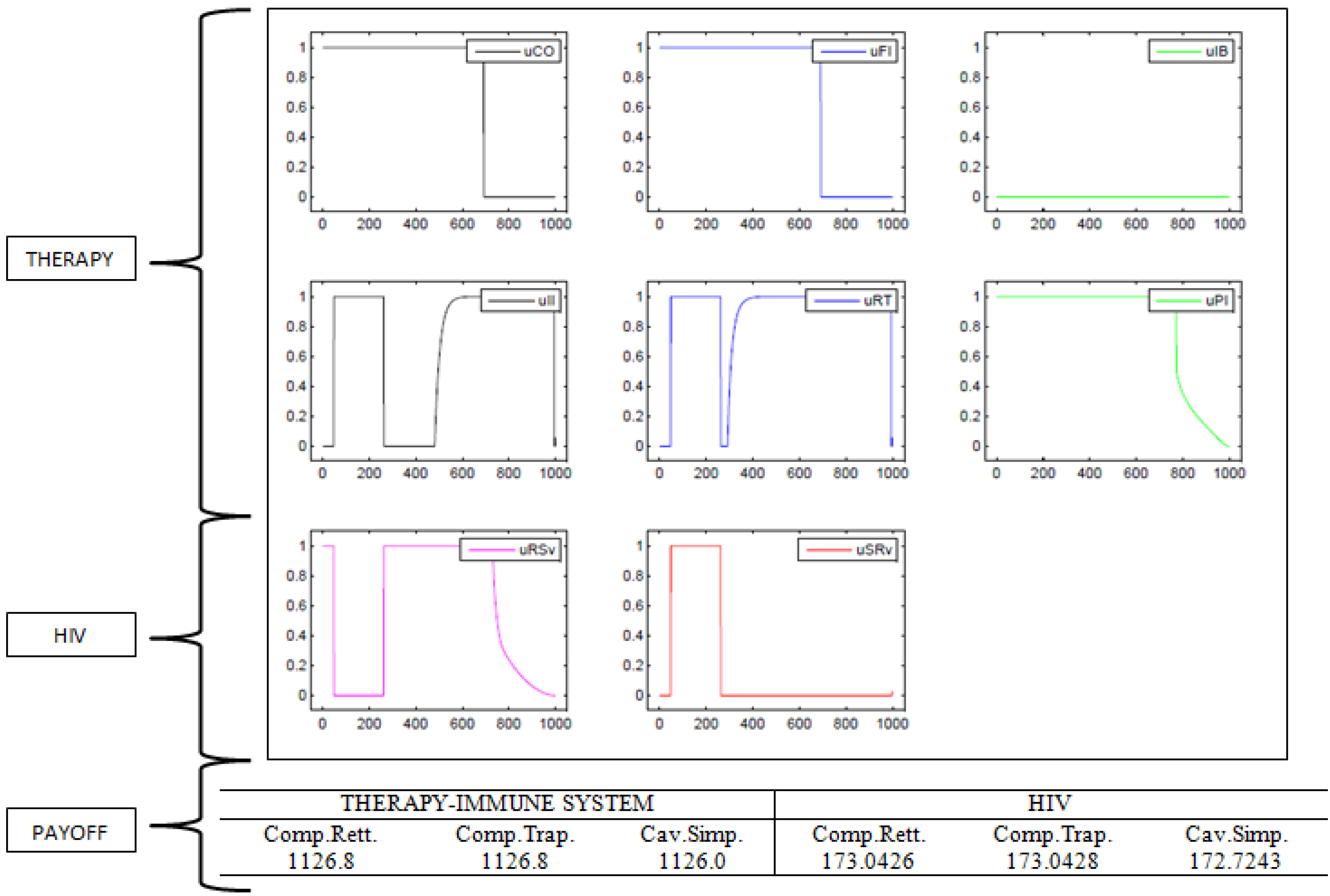
HIV mutation rate $u_{r,s}^v$ is maximum for the first 20 days then it decreases thanks to the combined action of therapy controls $u_{co},u_{fi}$ and $u_{pi}$. The reduction of $u_{r,s}^v$ involves the immediate increase of the sensitive-to-resistant viruses mutation rate ($u_{s,r}^v$) to the maximum level. This causes the necessity to use the controls $u_{ii}$ and $u_{rt}$ at the highest level till day 250 in order to reduce to zero mutations $u_{s,r}^v.$ Thanks to the prolonged therapy the latter remain at that null level until the end of the considered time interval. HIV attempts a further sting in the tail, by increasing the rate of mutation $u_{r,s}^v$ to the highest level. In the meantime controls $u_{ii}$ and $u_{rt}$ are brought to zero for a small time interval, while the controls $u_{co},u_{fi}$ and $u_{pi}$ continue to be used at their maximum level. Until the control $u_{r,s}^v$ remains at a high level, the controls $u_{ii}$ and $u_{rt}$ perform a gradual increase.

We can observe how the combined action of 5 drugs leads to a decrease of the mutation rate $u_{r,s}^v$, around day 700. It continues to decrease for the remaining 300 days, after which both the viruses mutation rates are null. Immune boosting ($u_{ib}$) continues to have a null dosage, for the same reasons seen in the concave instance.

The payoff for therapy and HIV are listed in the lower part of Figure 5. Due to the low toxicity of the drugs, the optimal immune system-therapy payoff turns to greater w.r.t. the one obtained in the concave instance, whilst the HIV payoff turns to be lower.

Figure 5. Equilibrium strategies and payoffs (nonconcave instance).

Figure 5. Equilibrium strategies and payoffs (nonconcave instance).

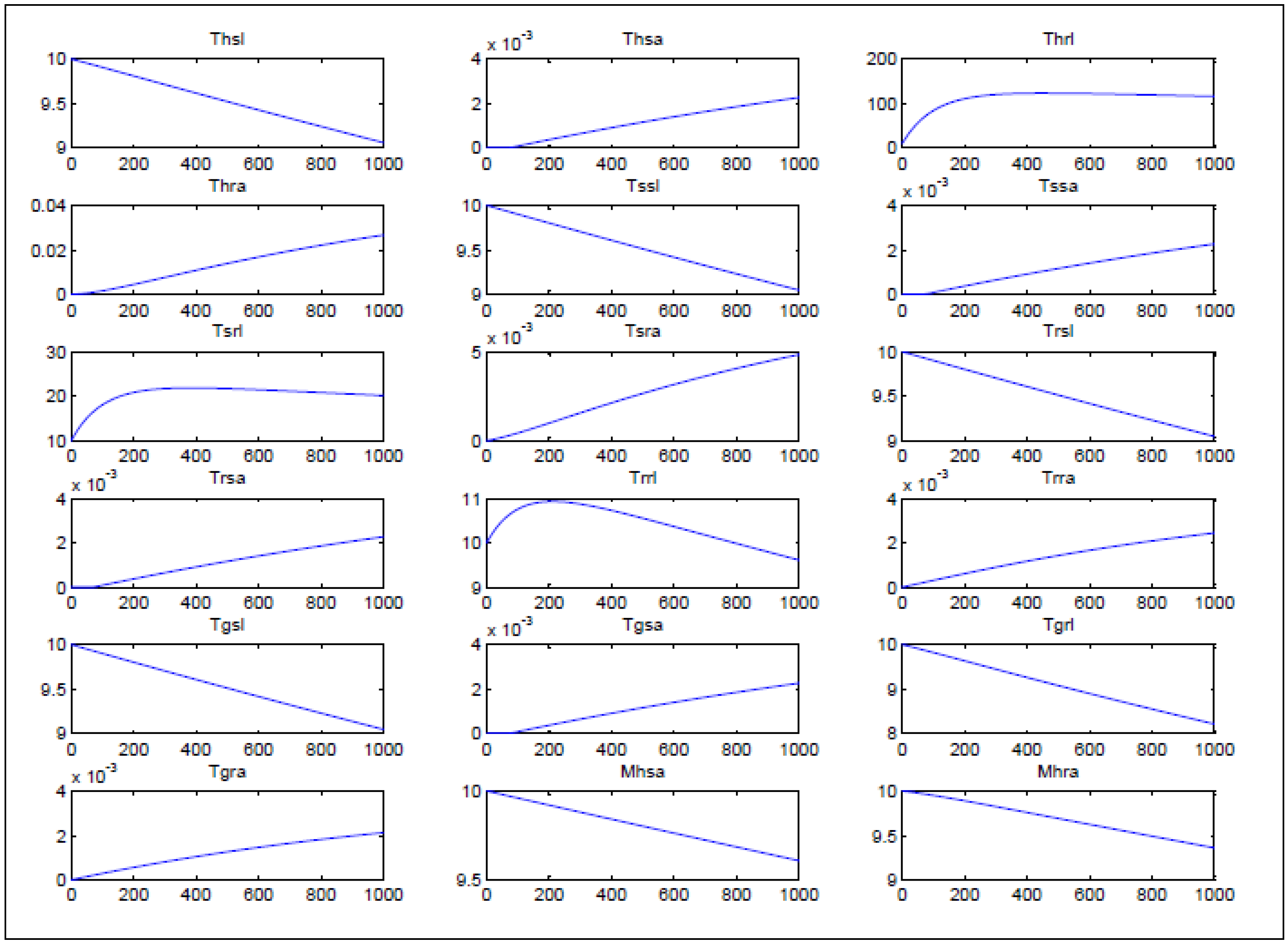
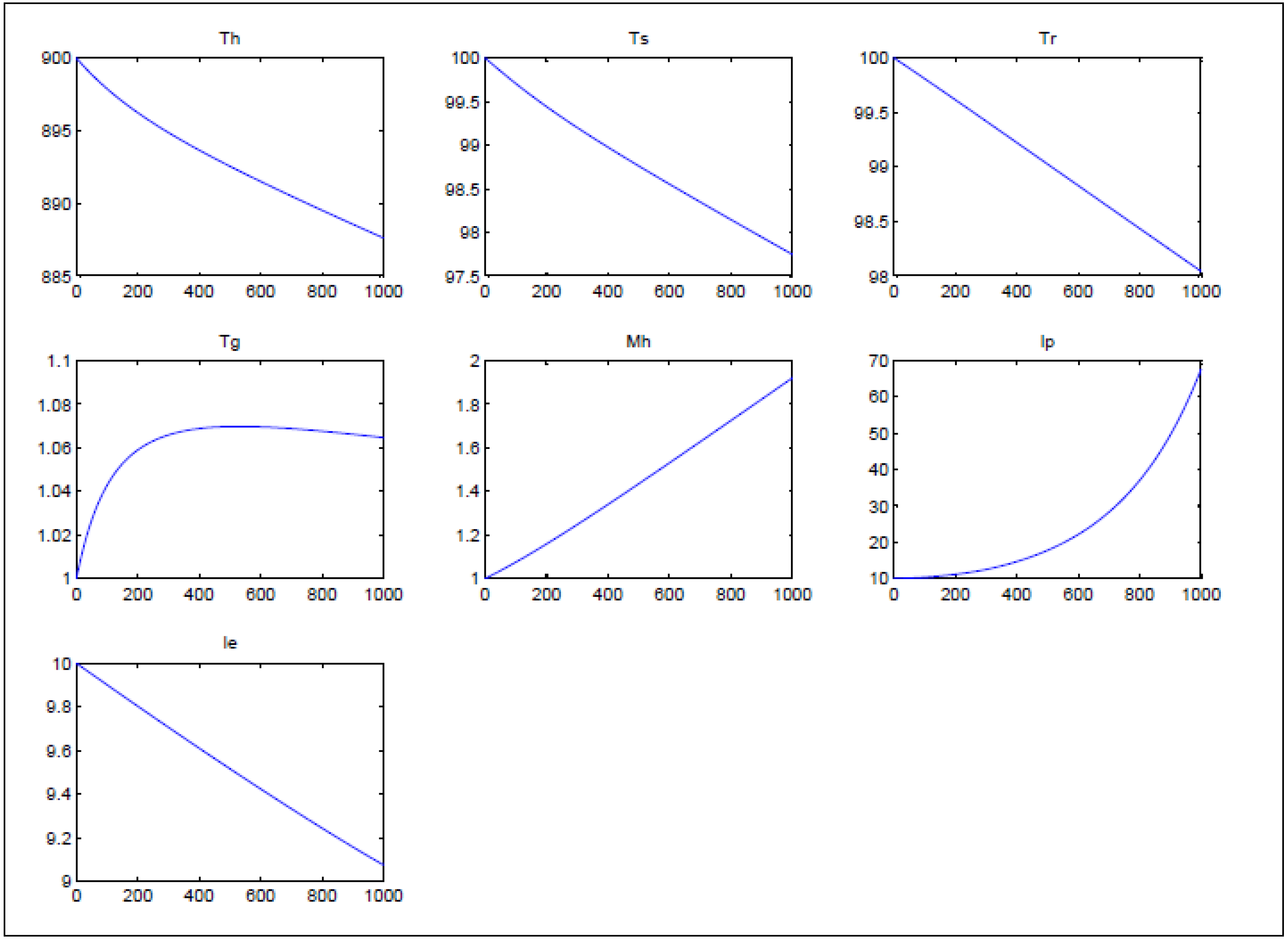
In Figure 6, Figure 7 and Figure 8 we report the dynamics of all 27 variable states. Note again that all optimal state functions are positive, so that the non-negativity constraints are fully satisfied. Although the drugs are not so effective, the lymphocytes count is high (around 800–900 $cells/m{m}^3$). Sensitive viruses population ($V_s$) becomes null around day 300, while resistant viruses population ($V_r$) goes to zero after 900 days.

Figure 6. Lymphocytes, macrophage and CTL dynamics (nonconcave instance).

Figure 6. Lymphocytes, macrophage and CTL dynamics (nonconcave instance).

Figure 7. Infected cells dynamics (nonconcave instance).

Figure 7. Infected cells dynamics (nonconcave instance).

Figure 8. Sensitive and resistant viruses dynamics (nonconcave instance).

Figure 8. Sensitive and resistant viruses dynamics (nonconcave instance).

5. Conclusions

We have considered the game theory approach in a medical-therapeutic context for HIV treatment. We have formulated a differential game which describes the interaction between the immune system of a patient and the virus action. In order to model the efficient HAART therapy, we have considered 27 state functions and eight controls (six for the therapy and two for HIV). We look for an open Loop Nash equilibrium in order to find a stable long-term coexistence between the two players.

The optimality necessary conditions lead to a system of 81 first order strongly non-linear differential equations. Once proved the existence and uniqueness of the solution of such a system, we have performed some numerical simulations in order to get enlightening results. Just for explanatory examples, we considered two specific instances. Mathematically speaking the two instances differ in the concavity properties of the Hamiltonians w.r.t. the related controls. From the medical point of view, the concave instance is characterized by very effective although highly toxic drugs, whereas the nonconcave instance is represented by low effective and moderately toxic drugs. We observe quite different behaviours in the therapy strategies according to the type of drugs used. And this, in our opinion, is very interesting, as our aim is to find a tool which can support the clinician when combining the different drugs in the HAART therapy. Having an idea of the dynamical reactions to a given biological effect can help to make the optimal therapeutic decision.

An immediate, although not trivial, prospect could be the analysis of the problem following the Hamilton-Jacobi-Bellman approach to find a time consistent Markovian Nash equilibrium [24].

Another possible further extension of this model could be obtained in matching the Game Theory approach with the Fuzzy system issue [25,26,27,28], paying attention to the unavoidable complexity increase.

References

- Moroni, M. AIDS, Se lo Conosci lo Eviti, 25 Anni di AIDS; Treccani: Firenze, Italy, 2007. [Google Scholar]
- Dybul, M.; Connors, M.; Fauci, A.; Paul, W. Immunology of HIV infection. In Fundamental Immunology, 5th ed.; Lippincott Williams & Wilkins: Philadelphia, PA, USA, 2003; pp. 1285–1318. [Google Scholar]
- Nachega, J.B.; Marconi, V.C.; van Zyl, G.U.; Gardner, E.M.; Preiser, W.; Hong, S.Y.; Mills, E.J.; Gross, R. HIV treatment adherence, drug resistance, virologic failure: Evolving concepts. Infect. Disord. Drug Targets 2011, 11, 167–174. [Google Scholar] [CrossRef] [PubMed]
- Joly, M.; Pinto, J.M. Role of mathematical modeling on the optimal control of HIV-1 pathogenesis. AIChE J. 2006, 52, 856–884. [Google Scholar] [CrossRef]
- Buratto, A.; Cesaretto, R.; Zamarchi, R. HIV Inside the Body: A Review of Mathematical Modeling; Padua University: Padua, Italy, 2015. [Google Scholar]
- Wu, J.; Zhang, M. A game theoretical approach to optimal control of dual drug delivery for HIV infection treatment. IEEE Trans. Syst. Man Cybern. B Cybern. 2010, 40, 694–702. [Google Scholar] [PubMed]
- Coppola, V.; Camus, O. Preventing without stigmatizing: The complex stakes of information on AIDS. Patient Educ. Couns. 2007, 67, 255–260. [Google Scholar] [CrossRef] [PubMed]
- Shonkwiler, R.W.; Herod, J. Mathematical Biology: An Introduction with Maple and Matlab; Springer Science & Business Media: New York, NY, USA, 2009; Volume 73. [Google Scholar]
- Nowak, M.A. Evolutionary Dynamics; Harvard University Press: Cambridge, MA, USA, 2006. [Google Scholar]
- Kirschner, D.E.; Webb, G. Immunotherapy of HIV-1 infection. J. Biol. Syst. 1998, 6, 71–83. [Google Scholar] [CrossRef]
- Caetano, M.A.; Yoneyama, T. Short and long period optimization of drug doses in the treatment of AIDS. An. Acad. Bras. Cienc. 2002, 74, 379–392. [Google Scholar] [CrossRef] [PubMed]
- Joshi, H.R. Optimal control of an HIV immunology model. Optim. Control Appl. Methods 2002, 23, 199–213. [Google Scholar] [CrossRef]
- Wodarz, D.; Nowak, M.A. Specific therapy regimes could lead to long-term immunological control of HIV. Proc. Natl. Acad. Sci. USA 1999, 96, 14464–14469. [Google Scholar] [CrossRef] [PubMed]
- Kirschner, D.; Perelson, A. A model for the immune system response to HIV: AZT treatment studies. Math. Popul. Dyn. Anal. Heterog. 1995, 1, 295–310. [Google Scholar]
- Wein, L.M.; Zenios, S.A.; Nowak, M.A. Dynamic multidrug therapies for HIV: A control theoretic approach. J. Theor. Biol. 1997, 185, 15–29. [Google Scholar] [CrossRef] [PubMed]
- Wein, L.M.; D’Amato, R.M.; Perelson, A.S. Mathematical analysis of antiretroviral therapy aimed at HIV-1 eradication or maintenance of low viral loads. J. Theor. Biol. 1998, 192, 81–98. [Google Scholar] [CrossRef] [PubMed]
- Haase, A.T.; Henry, K.; Zupancic, M.; Sedgewick, G.; Faust, R.A.; Melroe, H.; Cavert, W.; Gebhard, K.; Staskus, K.; Zhang, Z.Q.; et al. Quantitative image analysis of HIV-1 infection in lymphoid tissue. Science 1996, 274, 985–989. [Google Scholar] [CrossRef] [PubMed]
- Lenhart, S.; Workman, J.T. Optimal Control Applied to Biological Models; CRC Press: Boca Raton, FL, USA, 2007. [Google Scholar]
- Velichenko, V. A numerical method for solving optimal control problems. USSR Comput. Math. Math. Phys. 1966, 6, 34–50. [Google Scholar] [CrossRef]
- Velichenko, V.; Pritykin, D. Control of the medical treatment of AIDS. Autom. Remote Control 2006, 67, 493–511. [Google Scholar] [CrossRef]
- Velichenko, V.; Pritykin, D. Numerical methods of optimal control of the HIV-infection dynamics. J. Comput. Syst. Sci. Int. 2006, 45, 894–905. [Google Scholar] [CrossRef]
- Quarteroni, F.S.A.; Saleri, F. Calcolo Scientifico; Springer: New York, NY, USA, 2008. [Google Scholar]
- Niu, P.; Lyonsl, N.; Hsuz, A.; Grannemanz, G.R.; Hos, D.D. Ordered accumulation of mutations in HIV protease confers resistance to ritonavir. Nat. Med. 1996, 2, 760–766. [Google Scholar]
- Dockner, E. Differential Games in Economics and Management Science; Cambridge University Press: Cambridge, UK, 2000. [Google Scholar]
- Dalal, N.; Greenhalgh, D.; Mao, X. A stochastic model for internal HIV dynamics. J. Math. Anal. Appl. 2008, 341, 1084–1101. [Google Scholar] [CrossRef] [Green Version]
- Grégio, J.M.; Caetano, M.A.; Yoneyama, T. State estimation and optimal long period clinical treatment of HIV seropositive patients. An. Acad. Bras. Cienc. 2009, 81, 3–12. [Google Scholar] [CrossRef] [PubMed]
- Tan, W.Y.; Xiang, Z. Some state space models of HIV pathogenesis under treatment by anti-viral drugs in HIV-infected individuals. Math. Biosci. 1999, 156, 69–94. [Google Scholar] [CrossRef]
- Tuckwell, H.C.; Le Corfec, E. A stochastic model for early HIV-1 population dynamics. J. Theor. Biol. 1998, 195, 451–463. [Google Scholar] [CrossRef] [PubMed]
- Seierstad, A.; Sydsaeter, K. Optimal Control Theory with Economic Applications; North-Holland: Amsterdam, The Netherlands, 1987; Volume 20. [Google Scholar]
© 2015 by the authors; licensee MDPI, Basel, Switzerland. This article is an open access article distributed under the terms and conditions of the Creative Commons Attribution license (http://creativecommons.org/licenses/by/4.0/).
Share and Cite
MDPI and ACS Style
Buratto, A.; Cesaretto, R.; Zamarchi, R. HIV vs. the Immune System: A Differential Game. Mathematics 2015, 3, 1139-1170. https://doi.org/10.3390/math3041139
AMA Style
Buratto A, Cesaretto R, Zamarchi R. HIV vs. the Immune System: A Differential Game. Mathematics. 2015; 3(4):1139-1170. https://doi.org/10.3390/math3041139
Chicago/Turabian StyleBuratto, Alessandra, Rudy Cesaretto, and Rita Zamarchi. 2015. "HIV vs. the Immune System: A Differential Game" Mathematics 3, no. 4: 1139-1170. https://doi.org/10.3390/math3041139