
Solution of Excited Non-Linear Oscillators under Damping Effects Using the Modified Differential Transform Method

Abstract
:1. Introduction
2. Differential Transform Method
3. Forced Duffing Oscillator under Damping Effect
3.1. Example 1: Free Duffing Oscillator under Damping Effect
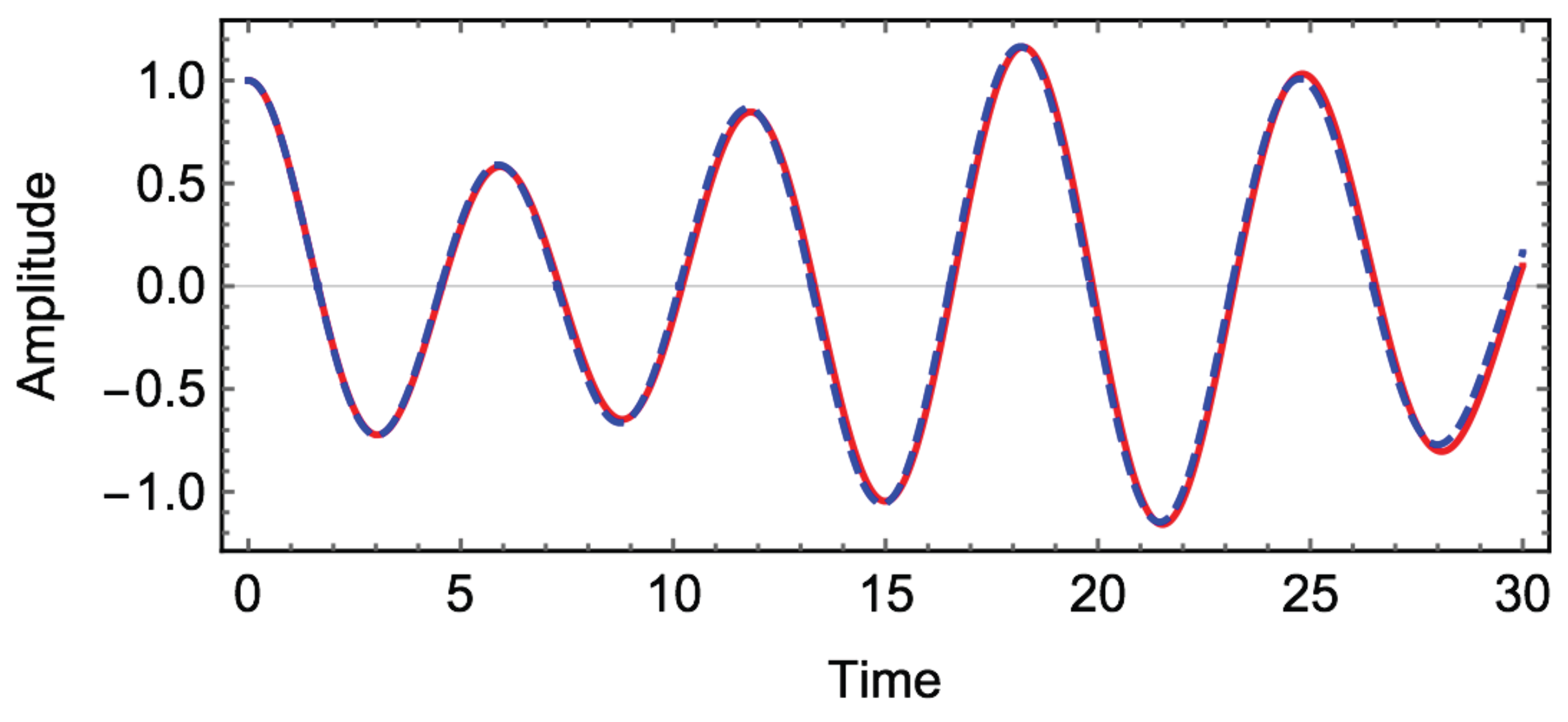
3.2. Example 2: Forced Nonlinear Duffing Oscillator with Damping Effect
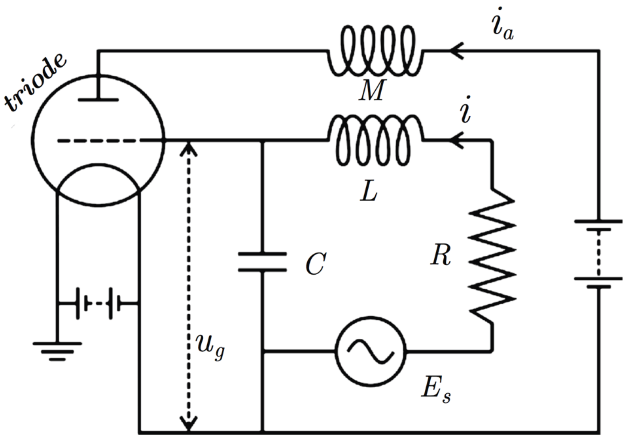
4. Forced van der Pol Oscillator under Damping Effect
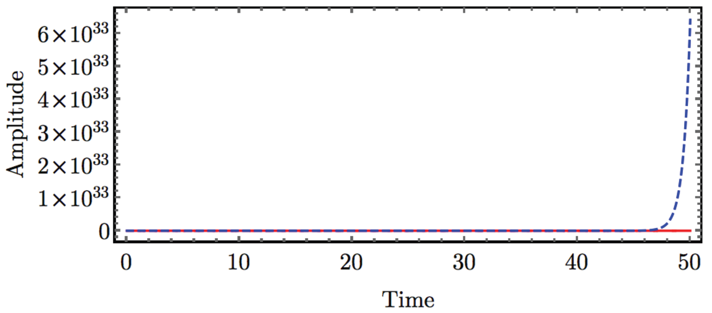
4.1. Example 3:
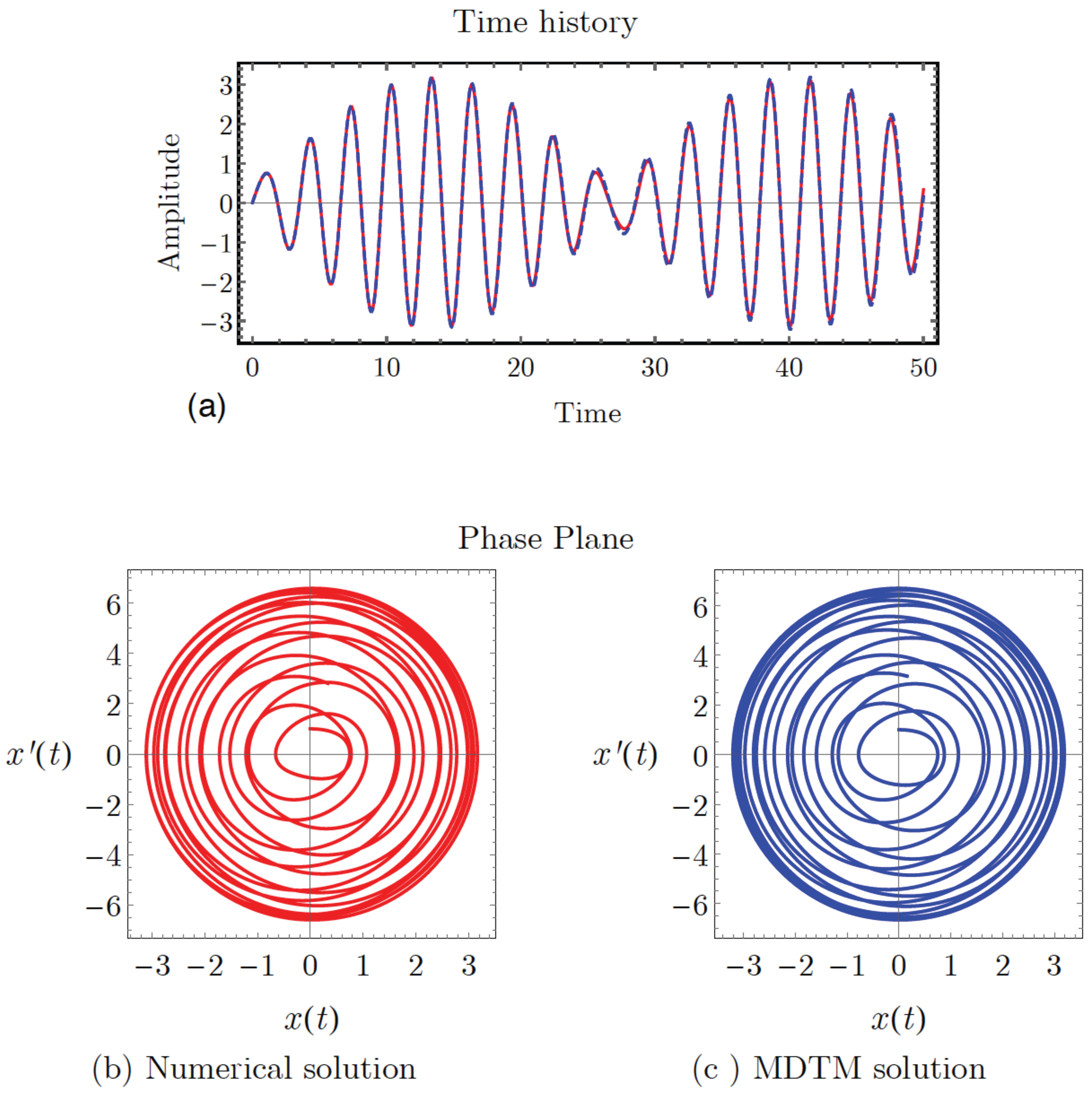
4.2. Example 4:
5. Conclusions
Conflicts of Interest
References
- Guckenheimer, J.; Holmes, P. Nonlinear Oscillations, Dynamical Systems and Bifurcations of Vector Fields; Springer-Verlag: New York, NY, USA, 1983. [Google Scholar]
- Ahmadian, M.T.; Mojahedi, M.; Moeenfard, H. Free vibration analysis of a nonlinear beam using homotopy and modified LindstedtPoincaré methods. J. Solid Mech. 2009, 1, 29–36. [Google Scholar]
- Bakhtiari-Nejad, F.; Nazari, M. Nonlinear vibration analysis of isotropic cantilever plate with viscoelastic laminate. Nonlinear Dyn. 2009, 56, 325–356. [Google Scholar] [CrossRef]
- Srinil, N.; Zanganeh, H. Modeling of coupled cross-flow/in-line vortex-induced vibrations using double Duffing and van der Pol oscillators. Ocean Eng. 2012, 53, 83–97. [Google Scholar] [CrossRef] [Green Version]
- Cartwright, M.L. Balthazar van der Pol. J. Lond. Math. Soc. 1960, 35, 367–376. [Google Scholar] [CrossRef]
- Cartwright, M.L. Van der Pols Equation for Relaxation Oscillations, in Contributions to the Theory of Nonlinear Oscillations II; Princeton Annals of Mathematics Studies 2; Princeton University Press: Princeton, NJ, USA, 1952; p. 318. [Google Scholar]
- Stumpers, F.L.H.M. Balth. van der Pols work on nonlinear circuits. IRE Trans. Circuit Theory 1960, 7, 366–367. [Google Scholar] [CrossRef]
- Van der Pol, B. A theory of the amplitude of free and forced triode vibrations. Radio Rev. 1920, 1, 701–710. [Google Scholar]
- Van der Pol, B. Relaxation Oscillations I. Phil. Mag. 1926, 2, 978–992. [Google Scholar] [CrossRef]
- Van der Pol, B. The nonlinear theory of electric oscillations. Proc. IRE 1934, 22, 1051–1086. [Google Scholar] [CrossRef]
- Nayfeh, A.H. Perturbation Methods; John Wiley: New York, NY, USA, 1973. [Google Scholar]
- Nayfeh, A.H.; Mook, D.T. Nonlinear Oscillations; John Wiley: New York, NY, USA, 1979. [Google Scholar]
- Nayfeh, A.H. Introduction to Perturbation Methods; Jhon Wiley: New York, NY, USA, 1981. [Google Scholar]
- Krylov, N.; Bogolioubov, N. Introduction to Nonlinear Mechanics; Princeton University Press: Princeton, NJ, USA, 1943. [Google Scholar]
- Bogolioubov, N.N.; Mitropolsky, Y.A. Asymptotic Methods in the Theory of Nonlinear Oscillations; Gordon and Breach: New York, NY, USA, 1961. [Google Scholar]
- Sanders, J.A.; Verhulst, F. Averaging Methods in Nonlinear Dynamical Systems; Springer-Verlag: New York, NY, USA, 1985. [Google Scholar]
- Zhou, J.K. Differential Transformation and Its Application for Electrical Circuits; Huazhong University Press: Wuhan, China, 1986. [Google Scholar]
- Mao, Q. Design of shaped piezoelectric modal sensors for cantilever beams with intermediate support by using differential transformation method. Appl. Acoust. 2012, 73, 144–149. [Google Scholar] [CrossRef]
- Rashidi, M.M.; Erfani, E. Analytical method for solving steady MHD convective and slip flow due to a rotating disk with viscous dissipation and Ohmic heating. Eng. Comput. 2012, 29, 562–579. [Google Scholar] [CrossRef]
- Rashidi, M.M.; Domairry, G. New analytical solution of the three dimensional Navier Stokes equations. Mod. Phys. Lett. B 2009, 23, 3147–3155. [Google Scholar] [CrossRef]
- Su, X.H.; Zheng, L.C. Approximate solutions to MHD Falkner Skan flow over permeable wall. Appl. Math. Mech. (Engl. Ed.) 2011, 32, 401–408. [Google Scholar] [CrossRef]
- Momani, S.; Odibat, Z.; Erturk, V.S. Generalized differential transform method for solving a space- and time-fractional diffusion-wave equation. Phys. Lett. A 2007, 370, 379–387. [Google Scholar] [CrossRef]
- Kangalgil, F.; Ayaz, F. Solitary wave solutions for the KdV and mKdV equations by differential transform method. Chaos Solitons Fractals 2009, 41, 464–472. [Google Scholar] [CrossRef]
- Biazar, J.; Eslami, M. Analytic solution for Telegraph equation by differential transform method. Phys. Lett. A 2010, 374, 2904–2906. [Google Scholar] [CrossRef]
- Hesam, S.; Nazemi, A.R.; Haghbin, A. Analytical solution for the Fokker Planck equation by differential transform method. Sci. Iran. 2012, 19, 1140–1145. [Google Scholar] [CrossRef]
- El-Shahed, M. Application of differential transform method to non-linear oscillatory systems. Commun. Nonlinear Sci. Numer. Simul. 2008, 13, 1714–1720. [Google Scholar] [CrossRef]
- Momani, S.; Erturk, V.S. Solutions of non-linear oscillators by the modified differential transform method. Comput. Math. Appl. 2008, 55, 833–842. [Google Scholar] [CrossRef]
- Yildirim, A.; Gokdogan, A.; Merdan, M. Chaotic systems via multistep differential transformation method. Can. J. Phys. 2012, 90, 391–406. [Google Scholar] [CrossRef]
- Mirzabeigy, A.; Yildirim, A. Approximate periodic solution for nonlinear jerk equation as a third-order nonlinear equation via modified differential transform method. Eng. Comput. 2014, 31, 622–633. [Google Scholar] [CrossRef]
- Erturk, V.S.; Yildirim, A.; Momani, S.; Khan, Y. The differential transform method and Padé approximants for a fractional population growth model. Int. J. Numer. Methods Heat Fluid Flow 2012, 22, 791–802. [Google Scholar] [CrossRef]
- Baker, G.A. Essentials of Padé Approximants; Academic Press: London, UK, 1975. [Google Scholar]
- Nourazar, S.; Mirzabeigy, A. Approximate solution for nonlinear Duffing oscillator with damping effect using the modified differential transform method. Sci. Iran. B 2013, 20, 364–368. [Google Scholar]
- Momani, S.; Ertürk, V.S. Solutions of non-linear oscillators by the modified differential transform method. Comput. Math. Appl. 2008, 55, 833–842. [Google Scholar] [CrossRef]


| Original Function | Transformed Function |
|---|---|
© 2016 by the author; licensee MDPI, Basel, Switzerland. This article is an open access article distributed under the terms and conditions of the Creative Commons by Attribution (CC-BY) license (http://creativecommons.org/licenses/by/4.0/).
Share and Cite
Abdelhafez, H.M. Solution of Excited Non-Linear Oscillators under Damping Effects Using the Modified Differential Transform Method. Mathematics 2016, 4, 11. https://doi.org/10.3390/math4010011
Abdelhafez HM. Solution of Excited Non-Linear Oscillators under Damping Effects Using the Modified Differential Transform Method. Mathematics. 2016; 4(1):11. https://doi.org/10.3390/math4010011
Chicago/Turabian StyleAbdelhafez, H. M. 2016. "Solution of Excited Non-Linear Oscillators under Damping Effects Using the Modified Differential Transform Method" Mathematics 4, no. 1: 11. https://doi.org/10.3390/math4010011