Inverse Eigenvalue Problems for Two Special Acyclic Matrices

Abstract

In this paper, we study two inverse eigenvalue problems (IEPs) of constructing two special acyclic matrices. The first problem involves the reconstruction of matrices whose graph is a path, from given information on one eigenvector of the required matrix and one eigenvalue of each of its leading principal submatrices. The second problem involves reconstruction of matrices whose graph is a broom, the eigen data being the maximum and minimum eigenvalues of each of the leading principal submatrices of the required matrix. In order to solve the problems, we use the recurrence relations among leading principal minors and the property of simplicity of the extremal eigenvalues of acyclic matrices.

1. Introduction

The problems of reconstruction of specially structured matrices from a prescribed set of eigen data are collectively known as inverse eigenvalue problems (IEPs). The level of difficulty of an IEP depends on the structure of the matrices which are to be reconstructed and on the type of eigen information available. M.T. Chu in [1] gave a detailed characterization of inverse eigenvalue problems. A few special types of inverse eigenvalue problems have been studied in [2,3,4,5,6,7,8]. Inverse problems for matrices with prescribed graphs have been studied in [9,10,11,12,13,14]. Inverse eigenvalue problems arise in a number of applications such as control theory, pole assignment problems, system identification, structural analysis, mass spring vibrations, circuit theory, mechanical system simulation and graph theory [1,12,15,16].

In this paper, we study two IEPs, namely IEPP (inverse eigenvalue problem for matrices whose graph is a path) and IEPB (inverse eigenvalue problem for matrices whose graph is a broom). Similar problems were studied in [5], for arrow matrices. The usual process of solving such problems involves the use of recurrence relations among the leading principal minors of $\lambda I-A$ where A is the required matrix. However, we have included graphs in our analysis by bringing in the requirement of constructing matrices which are described by graphs. In particular, we have considered paths and brooms. Thus, in addition to recurrence relations among leading principal minors, we have used spectral properties of acyclic matrices to solve the problems. Particularly, the strict interlacing of the eigenvalues in IEPB could be proved because of the fact that the minimal and maximal eigenvalues of an acyclic matrix are simple.

The paper is organized as follows : In Section 2, we discuss some preliminary concepts and clarify the notations used in the paper. In Section 3, we define the inverse problems to be studied, namely IEPP and IEPB. Section 4 deals with the analysis of IEPP, the main result being presented as Theorem 4. Section 5 deals with the analysis of IEPB, the main result being presented as Theorem 9. In Section 6, we present some numerical examples to illustrate the solutions of IEPP and IEPB.

2. Preliminary Concepts

Let V be a finite set and let P be the set of all subsets of V which have two distinct elements. Let $E\subset P$. Then $G=(V,E)$ is said to be a graph with vertex set V and edge set E. To avoid confusion, the vertex set of a graph G is denoted by $V(G)$ and the edge set is denoted by $E(G)$. Our choice of P implies that the graphs under consideration are free of multiple edges or loops and are undirected. If $u,v\in V$ and $\{u,v\}\in E$, then we say that $uv$ is an edge and u and v are then called adjacent vertices. The degree of a vertex u is the number of edges which are incident on u. A vertex of degree one is called a pendant vertex. A path P of G is a sequence of distinct vertices $v_1,v_2,\dots ,v_n$ such that consecutive vertices are adjacent. The path on n vertices is denoted by $P_n$. A graph is said to be connected if there exists a path between every pair of its vertices. A cycle is a connected graph in which each vertex is adjacent to exactly two other vertices. A connected graph without any cycles is called a tree.

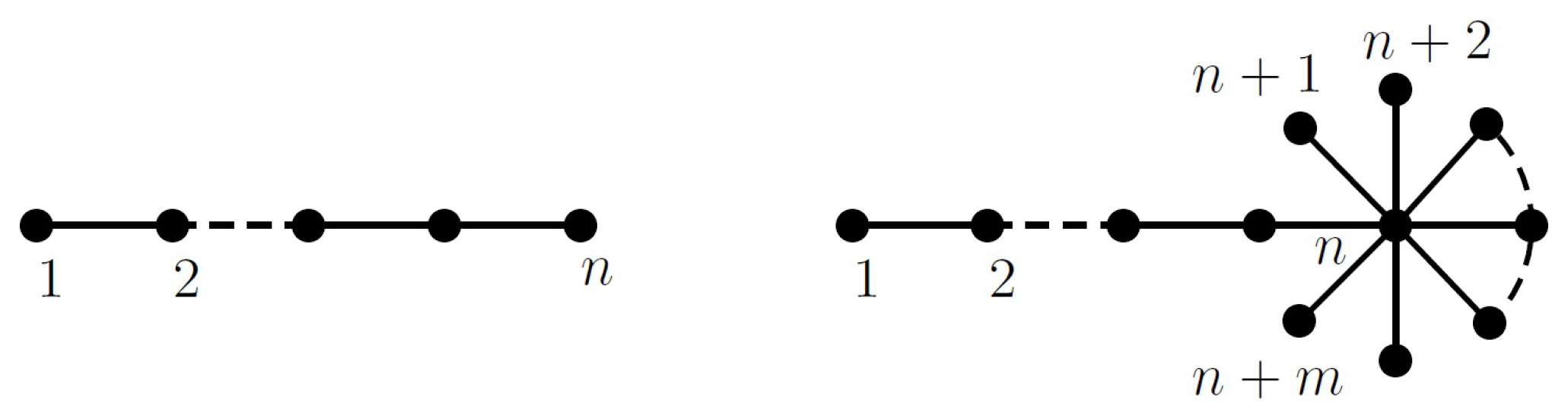
Given an $n\times n$ symmetric matrix A, the graph of A, denoted by $G(A)$, has vertex set $V(G)=\{1,2,3,\dots ,n\}$ and edge set $\{ij:i\ne j,a_{ij}\ne 0\}$. For a graph G with n vertices, $S(G)$ denotes the set of all $n\times n$ symmetric matrices which have G as their graph. A matrix whose graph is a tree is called an acyclic matrix. Some simple examples of acyclic matrices are the matrices whose graphs are paths or brooms (Figure 1).

Throughout this paper, we shall use the following notation:

• Matrix of a path $P_n$ will be a tridiagonal matrix with non zero off-diagonal entries :

  $$A_n={\left(\begin{array}{cccccc}{a}_1& b_1& 0& \dots & 0& 0\\ b_1& a_2& b_2& \dots & 0& 0\\ 0& b_2& a_3& \ddots & 0& 0\\ ⋮& ⋮& \ddots & \ddots & \ddots & ⋮\\ 0& 0& 0& \ddots & a_{n-1}& b_{n-1}\\ 0& 0& 0& \dots & b_{n-1}& a_n\end{array}\right)}_{n\times n},$$

  where the $b_i$s are non-zero.
• Matrix of a broom $B_{n+m}$ will be of the following form:

  $$A_{n+m}={\left(\begin{array}{cccccccccc}{a}_1& b_1& 0& \dots & 0& 0& 0& 0& \dots & 0\\ b_1& a_2& b_2& \dots & 0& 0& 0& 0& \dots & 0\\ 0& b_2& a_3& \ddots & 0& 0& 0& 0& \dots & 0\\ ⋮& ⋮& \ddots & \ddots & ⋮& ⋮& ⋮& ⋮& ⋮& ⋮\\ 0& 0& 0& \dots & a_{n-1}& b_{n-1}& 0& 0& \dots & 0\\ 0& 0& 0& \dots & b_{n-1}& a_n& b_n& b_{n+1}& \dots & b_{n+m-1}\\ 0& 0& 0& \dots & 0& b_n& a_{n+1}& 0& \dots & 0\\ 0& 0& 0& \dots & 0& b_{n+1}& 0& a_{n+2}& \ddots & 0\\ ⋮& ⋮& ⋮& ⋮& ⋮& ⋮& ⋮& \ddots & \ddots & ⋮\\ 0& 0& 0& \dots & 0& b_{n+m-1}& 0& 0& \dots & a_{n+m}\end{array}\right)}_{(n+m)\times (n+m)},$$

  where the $b_i$s are non zero.
• $A_i$ will denote the ith leading principal submatrix of the required matrix ($A_n$ or $A_{n+m}$).
• $P_i(\lambda )=det(\lambda I_i-A_i)$, $i=1,2,\dots ,n$ (respectively $i=1,2,\dots n+m$) i.e., the ith leading principal minor of $\lambda I_n-A_n$ (respectively $\lambda I_{n+m}-A_{n+m}$), $I_i$ being the identity matrix of order i. For the sake of writing the recurrence relations with ease, we define $P_0(\lambda )=1,b_0=0$.

3. IEPs to be Studied

In this paper we shall study the following two inverse eigenvalue problems :

IEPP Given n real numbers ${\lambda }_j,1\le j\le n$ and a real vector $X_n={(x_1,x_2,\dots ,x_n)}^T$ find an $n\times n$ matrix $A_n\in S(P_n)$ such that ${\lambda }_j$ is an eigenvalue of $A_j$, $j=1,2,\dots ,n$ and $({\lambda }_n,X_n)$ is an eigenpair of $A_n$.

IEPB Given $2n+2m-1$ real numbers ${\lambda }_1^{(j)},1\le j\le n+m$ and ${\lambda }_j^{(j)},2\le j\le n+m$, find an $(n+m)\times (n+m)$ matrix $A_{n+m}\in S(B_{n+m})$ such that ${\lambda }_1^{(j)}$ and ${\lambda }_j^{(j)}$ are respectively the minimal and maximal eigenvalues of $A_j$, $j=1,2,\dots ,n+m$.

4. Solution of IEPP

The following Lemma gives the relation between successive leading principal minors of $\lambda I_n-A_n$:

Lemma 1. 

The sequence ${\{P_j(\lambda )=det(\lambda I_j-A_j)\}}_{j=1}^n$ of characteristic polynomials of $A_j$ satisfies the following recurrence relations:

• $P_1(\lambda )=(\lambda -a_1)$
• $P_j(\lambda )=(\lambda -a_j)P_{j-1}(\lambda )-b_{j-1}^2{P}_{j-2}(\lambda )$, $2\le j\le n$.

Here $A_j$ denotes the jth leading principal submatrix of $A_n$, the matrix corresponding to the path on n vertices.

Lemma 2. 

For any $\lambda \in \mathbb{R}$ and $1\le j\le n$, $P_j(\lambda )$ and $P_{j+1}(\lambda )$ cannot be simultaneously zero.

Proof. 

If $P_1(\lambda )=0=P_2(\lambda )$, then $(\lambda -a_2)P_1(\lambda )-b_1^2=0$, which implies $b_1=0$, but this contradicts the restriction on $A_n$ that $b_1\ne 0$. Once again, for $2<j\le n$, if $P_{j-1}(\lambda )=0=P_j(\lambda )$, then the recurrence relation (ii) from Lemma 1, $(\lambda -a_{j+1})P_j(\lambda )-b_j^2{P}_{j-1}(\lambda )=0$, which gives $P_{j-1}(\lambda )=0$. This will in turn imply that $P_{j-2}(\lambda )=0$. Thus, we will end up with $P_2(\lambda )=0$, implying that $b_1=0$ which is a contradiction. □

Lemma 3. 

If $X={(x_1,x_2,\dots ,x_n)}^T$ is an eigenvector of $A_n$ corresponding to an eigenvalue λ, then $x_1\ne 0$ and the components of this eigenvector are given by

$$x_j={\displaystyle \frac{P_{j-1}(\lambda )}{{\prod }_{i=1}^{j-1}{b}_i}}{x}_1,j=2,3,\dots ,n.$$

Proof. 

Since $(\lambda ,X)$ is an eigenpair of $A_n$, we have $A_{n}X=\lambda X$. Comparing the first $n-1$ rows of this matrix equation on both sides, we have

$$(a_1-\lambda )x_1+b_1{x}_2=0,$$

(1)

$$b_{j-1}{x}_{j-1}+(a_j-\lambda )x_j+b_j{x}_{j+1}=0,j=2,\dots ,n-1.$$

(2)

By the second recurrence relation from Lemma 1,

$$P_j(\lambda )=(\lambda -a_j)P_{j-1}(\lambda )-b_{j-1}^2{P}_{j-2}(\lambda ),j=2,3,\dots ,n.$$

(3)

We define the quantities $v_1,v_2,\dots ,v_n$ as

$$v_1=x_1,v_j=x_j\prod _{i=1}^{j-1}{b}_i,2\le j\le n.$$

Multiplying Equation (2) by ${\prod }_{i=1}^{j-1}{b}_i$, we get

$$\begin{array}{cc}& b_{j-1}{x}_{j-1}\prod _{i=1}^{j-1}{b}_i+(a_j-\lambda )x_j\prod _{i=1}^{j-1}{b}_i+b_j{x}_{j+1}\prod _{i=1}^{j-1}{b}_i=0\hfill \\ \hfill \Rightarrow & b_{j-1}^2{v}_{j-1}+(a_j-\lambda )v_j+v_{j+1}=0,\hfill \end{array}$$

which gives

$$v_{j+1}=(\lambda -a_j)v_j-b_{j-1}^2{v}_{j-1},j=2,3,\dots ,n-1.$$

(4)

Now, from Equation (1), we have $v_2=(\lambda -a_1)x_1=x_1{P}_1(\lambda )$. Again from Equation (4),

$$v_3=(\lambda -a_2)v_2-b_1^2{v}_1=x_1\{(\lambda -a_2)P_1(\lambda )-b_1^2\}=x_1{P}_2(\lambda ).$$

Proceeding this way, we see that $v_{j+1}=x_1{P}_j(\lambda ),j=1,2,\dots ,n-1$ which can also be written as $v_j=x_1{P}_{j-1}(\lambda ),j=2,3,\dots ,n$. This further implies that

$$x_j={\displaystyle \frac{P_{j-1}(\lambda )}{{\prod }_{i=1}^{j-1}{b}_i}}{x}_1,j=2,3,\dots ,n.$$

(5)

Since X is an eigenvector, $X\ne 0$. If $x_1=0$, then from Equation (5), we see that all the other components of X become zero. Thus, $x_1\ne 0$. □

Theorem 4. 

The IEPP has a unique solution if and only if $x_j\ne 0$ for all $j=1,2,\dots ,n$. The unique solution is given by

$$a_1={\lambda }_1,a_j={\lambda }_j-{\displaystyle \frac{b_{j-1}^2{P}_{j-2}({\lambda }_j)}{P_{j-1}({\lambda }_j)}},j=2,\dots ,n$$

$$b_1={\displaystyle \frac{x_1}{x_2}}{P}_1({\lambda }_n)and{b}_{j-1}={\displaystyle \frac{x_1{P}_{j-1}({\lambda }_n)}{{\displaystyle x_j\prod _{i=1}^{j-2}{b}_i}}},j=3,4,\dots ,n.$$

Proof. 

Let $x_j\ne 0$ for all $j=1,2,\dots ,n$. As per the conditions of IEPP, ${\lambda }_j$ is an eigenvalue of $A_j$ for each $j=1,2,\dots ,n$. Thus, $P_1({\lambda }_1)=0\Rightarrow a_1={\lambda }_1$.

$$\begin{array}{cc}& P_j({\lambda }_j)=0\hfill \\ \hfill \Rightarrow & ({\lambda }_j-a_j)P_{j-1}({\lambda }_j)-b_{j-1}^2{P}_{j-2}({\lambda }_j)=0\hfill \\ \hfill \Rightarrow & a_j={\lambda }_j-{\displaystyle \frac{b_{j-1}^2{P}_{j-2}({\lambda }_j)}{P_{j-1}({\lambda }_j)}},\hfill \end{array}$$

(6)

which gives the expression for calculating $a_j$. The expression is valid as $P_{j-1}({\lambda }_j)\ne 0$, because by Lemma 2, $P_{j-1}({\lambda }_j)$ and $P_j({\lambda }_j)$ cannot be simultaneously zero.

Now, since $({\lambda }_n,X)$ is an eigenpair of $A_n$, so by Equation (5), $x_j={\displaystyle \frac{P_{j-1}({\lambda }_n)}{{\prod }_{i=1}^{j-1}{b}_i}}{x}_1,$ which implies that

$$b_1={\displaystyle \frac{x_1}{x_2}}{P}_1({\lambda }_n)\text{and}{b}_{j-1}={\displaystyle \frac{x_1{P}_{j-1}({\lambda }_n)}{x_j{\prod }_{i=1}^{j-2}{b}_i}}.$$

(7)

Since $x_j\ne 0\text{hence}\text{it}\text{follows}\text{that}$, $P_{j-1}({\lambda }_n)\ne 0$. Hence the above expression for $b_{j-1}$ is valid and $b_{j-1}\ne 0$ for all $j=2,3,\dots ,n$. Successive use of Equations (6) and (7) will give us the values of $a_j$ and $b_{j-1}$ for $j=1,2,\dots ,n$.

Conversely, if there exists a unique solution for IEPP, then since X is an eigenvector of $A_n$, so by Lemma 3, $x_1\ne 0$. The existence of a solution implies that $b_{j-1}\ne 0$ for $j=2,3,\dots ,n$. It then follows from the expressions in Equation (7) that $x_j\ne 0$ for $j=2,3,\dots ,n$. □

5. Solution of IEPB

Lemma 5. 

Let $P(\lambda )$ be a monic polynomial of degree n with all real zeros and ${\lambda }_{min}$ and ${\lambda }_{max}$ be the minimal and maximal zero of P respectively.

• If $\mu <{\lambda }_{min}$, then ${(-1)}^{n}P(\mu )>0$.
• If $\mu >{\lambda }_{max}$, then $P(\mu )>0$.

The proof immediately follows after expressing the polynomial as a product of its linear factors.

Lemma 6. 

If T is a tree, then the minimal and maximal eigenvalues of any matrix $A\in S(T)$ are simple i.e., of multiplicity one. [Corollary 6 of Theorem 2 in [17]]

In other words, this Lemma says that the minimal and maximal eigenvalues of an acyclic matrix are simple. Again, since for each j, the leading principal submatrix $A_j$ corresponds to a tree so by Lemma 6 the minimal and maximal eigenvalues of $A_j$ must be simple i.e., in particular ${\lambda }_1^{(j)}\ne {\lambda }_j^{(j)}$.

Lemma 7. 

The sequence ${\{P_j(\lambda )=det(\lambda I_j-A_j)\}}_{j=1}^{n+m}$ of characteristic polynomials of $A_j$ satisfies the following recurrence relations:

• $P_1(\lambda )=(\lambda -a_1)$.
• $P_j(\lambda )=(\lambda -a_j)P_{j-1}(\lambda )-b_{j-1}^2{P}_{j-2}(\lambda )$, $2\le j\le n+1$.
• ${\displaystyle P_{n+j}(\lambda )=(\lambda -a_{n+j})P_{n+j-1}(\lambda )-b_{n+j-1}^2{P}_{n-1}(\lambda )\prod _{i=1}^{j-1}(\lambda -a_{n+i}),2\le j\le m}$.

Lemma 8. 

For any $\lambda \in \mathbb{R}$ and $1\le j\le n$, $P_j(\lambda )$ and $P_{j+1}(\lambda )$ cannot be simultaneously zero.

Proof. 

Same as Lemma 2. □

By Cauchy’s interlacing theorem ([14,18]), the eigenvalues of a symmetric matrix and those of any of its principal submatrix interlace each other. Thus, ${\lambda }_1^{(j)}$’s and ${\lambda }_j^{(j)}$’s must satisfy:

$${\lambda }_1^{(n+m)}\le {\lambda }_1^{(n+m-1)}\le \dots \le {\lambda }_1^{(2)}\le {\lambda }_1^{(1)}\le {\lambda }_2^{(2)}\le {\lambda }_3^{(3)}\le \dots \le {\lambda }_{n+m-1}^{(n+m-1)}\le {\lambda }_{n+m}^{(n+m)}.$$

Each diagonal element $a_i$ is also a $1\times 1$ principal submatrix of A. Hence ${\lambda }_1^j\le a_i\le {\lambda }_j^{(j)},1\le i\le j$. Since ${\lambda }_1^{(j)}$ and ${\lambda }_j^{(j)}$ are the minimal and maximal eigenvalues of $A_j$, so $P_j({\lambda }_1^{(j)})=0$ and $P_j({\lambda }_j^{(j)})=0$. We need to solve these equations successively using the recurrence relations in Lemma 1. For $j=1$, $P_1({\lambda }_1^{(1)})=0\Rightarrow a_1={\lambda }_1^{(1)}$. For $j=2$, $P_2({\lambda }_1^{(2)})=0,P_2({\lambda }_2^{(2)})=0$ which imply that

$$a_2={\displaystyle \frac{{\lambda }_2^{(2)}{P}_1({\lambda }_2^{(2)})-{\lambda }_1^{(2)}{P}_1({\lambda }_1^{(2)})}{P_1({\lambda }_2^{(2)})-P_1({\lambda }_1^{(2)})}},b_1^2={\displaystyle \frac{({\lambda }_2^{(2)}-{\lambda }_1^{(2)})P_1({\lambda }_1^{(2)})P_1({\lambda }_2^{(2)})}{P_1({\lambda }_1^{(2)})-P_1({\lambda }_2^{(2)})}}.$$

$a_2$ will always exist as the denominator in the above expression for $a_2$ can never be zero. We have ${\lambda }_1^{(2)}\ne {\lambda }_2^{(2)}$ and so if $P_1({\lambda }_2^{(2)})=P_1({\lambda }_1^{(2)})$, then by Rolle’s theorem ∃$c\in ({\lambda }_1^{(2)},{\lambda }_2^{(2)})$ such that $P_1^{\prime }(c)=0\Rightarrow 1=0$, which is not possible. Thus, $P_1({\lambda }_2^{(2)})-P_1({\lambda }_1^{(2)})\ne 0$. Also, by Lemma 5, ${(-1)}^1{P}_1({\lambda }_1^{(2)})\ge 0$ and so the expression for $b_1^2$ is non-negative and so we can get real values of $b_1$.

Now for $3\le j\le n$, we have

$$P_j({\lambda }_1^{(j)})=0,P_j({\lambda }_j^{(j)})=0,$$

which gives

$$a_j{P}_{j-1}({\lambda }_1^{(j)})+b_{j-1}^2{P}_{j-2}({\lambda }_1^{(j)})-{\lambda }_1^{(j)}{P}_{j-1}({\lambda }_1^{(j)})=0,$$

$$a_j{P}_{j-1}({\lambda }_j^{(j)})+b_{j-1}^2{P}_{j-2}({\lambda }_j^{(j)})-{\lambda }_j^{(j)}{P}_{j-1}({\lambda }_j^{(j)})=0.$$

Let $D_j$ denote the determinant of the coefficient matrix of the above system of linear equations in $a_j$ and $b_{j-1}^2$. Then $D_j=P_{j-1}({\lambda }_1^{(j)})P_{j-2}({\lambda }_j^{(j)})-P_{j-1}({\lambda }_j^{(j)})P_{j-2}({\lambda }_1^{(j)})$. If $D_j\ne 0$, then the system will have a unique solution, given by

$$\begin{array}{cc}& a_j={\displaystyle \frac{{\lambda }_1^{(j)}{P}_{j-1}({\lambda }_1^{(j)})P_{j-2}({\lambda }_j^{(j)})-{\lambda }_j^{(j)}{P}_{j-1}({\lambda }_j^{(j)})P_{j-2}({\lambda }_1^{(j)})}{D_j}},\hfill \\ & b_{j-1}^2={\displaystyle \frac{({\lambda }_j^{(j)}-{\lambda }_1^{(j)})P_{j-1}({\lambda }_1^{(j)})P_{j-1}({\lambda }_j^{(j)})}{D_j}}.\hfill \end{array}$$

(8)

We claim that the expression for $b_{j-1}^2$ in RHS is non negative. This follows from Lemma 5. Since ${\lambda }_1^{(j)}\le {\lambda }_1^{(j-1)}$ and ${\lambda }_{j-1}^{(j-1)}\le {\lambda }_j^{(j)}$, so by Lemma 5,

$${(-1)}^{j-1}{D}_j={(-1)}^{(j-1)}{P}_{j-1}({\lambda }_1^{(j)})P_{j-2}({\lambda }_j^{(j)})+{(-1)}^{j-2}{P}_{j-2}({\lambda }_1^{(j)})P_{j-1}({\lambda }_j^{(j)})\ge 0.$$

In addition, by Lemma 2, $P_j({\lambda }_1^{(j)})$ and $P_{j-1}({\lambda }_1^{(j)})$ cannot be simultaneously zero. Thus, $P_{j-1}({\lambda }_1^{(j)})\ne 0$. Similarly, $P_{j-1}({\lambda }_j^{(j)})\ne 0$. This implies that ${\lambda }_1^{(j)}\ne {\lambda }_1^{(j-1)}$ and ${\lambda }_j^{(j)}\ne {\lambda }_{j-1}^{j-1}$. Thus, we can get non-zero real values of $b_{j-1}$ from Equation (8) if and only if ${\lambda }_1^{(j)}<{\lambda }_1^{(j-1)}$ and ${\lambda }_{j-1}^{(j-1)}<{\lambda }_j^{(j)}$ for all $j=2,3,\dots ,n$.

Now, if $D_j=0$, then ${(-1)}^{j-1}{D}_j=0$ i.e., ${(-1)}^{(j-1)}{P}_{j-1}({\lambda }_1^{(j)})P_{j-2}({\lambda }_j^{(j)})+{(-1)}^{j-2}{P}_{j-2}({\lambda }_1^{(j)})P_{j-1}({\lambda }_j^{(j)})=0$. Since both the terms in this sum are non negative, we must have $P_{j-1}({\lambda }_1^{(j)})P_{j-2}({\lambda }_j^{(j)})=0$ and $P_{j-2}({\lambda }_1^{(j)})P_{j-1}({\lambda }_j^{(j)})=0$. However, from Lemma 2, $P_{j-1}(\lambda )$ and $P_{j-2}(\lambda )$ cannot be simultaneously zero. In addition, $P_j(\lambda )$ and $P_{j-1}(\lambda )$ cannot be simultaneously zero. Thus, the only possibility is that $P_{j-2}({\lambda }_1^{(j)})=P_{j-2}({\lambda }_j^{(j)})=0$. However, this will then imply that $a_j={\lambda }_1^{(j)}={\lambda }_j^{(j)}$, which is not possible as by Lemma 6 ${\lambda }_1^{(j)}\ne {\lambda }_j^{(j)}$. Thus, $D_j\ne 0$ for all $j=2,3,\dots ,n$.

Again, ${\lambda }_1^{(n+j)}$ and ${\lambda }_{n+j}^{(n+j)}$ are the eigenvalues of $A_{n+j}$ and so $P_{n+j}({\lambda }_1^{(n+j)})=0$ and $P_{n+j}({\lambda }_{n+j}^{(n+j)})=0$. Hence,

$$\begin{array}{c}\hfill ({\lambda }_1^{(n+j)}-a_{n+j})P_{n+j-1}({\lambda }_1^{(n+j)})-b_{n+j-1}^2{P}_{n-1}({\lambda }_1^{(n+j)})\prod _{i=1}^{j-1}({\lambda }_1^{(n+j)}-a_{n+i})=0,\\ \hfill ({\lambda }_{n+j}^{(n+j)}-a_{n+j})P_{n+j-1}({\lambda }_{n+j}^{(n+j)})-b_{n+j-1}^2{P}_{n-1}({\lambda }_{n+j}^{(n+j)})\prod _{i=1}^{j-1}({\lambda }_{n+j}^{(n+j)}-a_{n+i})=0.\end{array}$$

(9)

so we get a system of equations linear in $a_{n+j}$ and $b_{n+j-1}^2.$

$$\begin{array}{c}\hfill a_{n+j}{P}_{n+j-1}({\lambda }_1^{(n+j)})+b_{n+j-1}^2{P}_{n-1}({\lambda }_1^{(n+j)})\prod _{i=1}^{j-1}({\lambda }_1^{(n+j)}-a_{n+i})={\lambda }_1^{(n+j)}{P}_{n+j-1}({\lambda }_1^{(n+j)}),\\ \hfill a_{n+j}{P}_{n+j-1}({\lambda }_{n+j}^{(n+j)})+b_{n+j-1}^2{P}_{n-1}({\lambda }_{n+j}^{(n+j)})\prod _{i=1}^{j-1}({\lambda }_{n+j}^{(n+j)}-a_{n+i})={\lambda }_{n+j}^{(n+j)}{P}_{n+j-1}({\lambda }_{n+j}^{(n+j)}).\end{array}$$

(10)

We first investigate the conditions under which the coefficient matrix of the above system is singular. By Cauchy’s interlacing property, we have

$${\lambda }_1^{(n+j)}\le {\lambda }_1^{(n+j-1)}\le \dots \le {\lambda }_1^{(n+1)}\le a_{n+i}\le {\lambda }_{n+1}^{(n+1)}\le \dots {\lambda }_{n+j-1}^{(n+j-1)}\le {\lambda }_{n+j}^{(n+j)},\text{for}\text{all}i=1,2,\dots ,m.$$

(11)

Thus, ${\displaystyle \prod _{i=1}^{j-1}({\lambda }_{n+j}^{(n+j)}-a_{n+i})\ge 0}$ and ${\displaystyle {(-1)}^{j-1}\prod _{i=1}^{j-1}({\lambda }_1^{(n+j)}-a_{n+i})\ge 0}$. Let $D_{n+j}$ be the determinant of the coefficient matrix of Equation (10). Then,

$$\begin{array}{cc}\hfill {(-1)}^{n+j-1}{D}_{n+j}=& {(-1)}^{n+j-1}{P}_{n+j-1}({\lambda }_1^{(n+j)})P_{n-1}({\lambda }_{n+j}^{(n+j)})\prod _{i+1}^{j-1}({\lambda }_{n+j}^{(n+j)}-a_{n+i}),\hfill \\ & +{(-1)}^{n+j-2}{P}_{n+j-1}({\lambda }_{n+j}^{(n+j)})P_{n-1}({\lambda }_1^{(n+j)})\prod _{i=1}^{j-1}({\lambda }_1^{(n+j)}-a_{n+i}).\hfill \end{array}$$

As a consequence of Lemma 5, both the products in the LHS are non-negative and so ${(-1)}^{n+j-1}{D}_{n+j}\ge 0$ for all $j=1,2,\dots ,m$. Thus, $D_{n+j}$ will vanish if and only if ${(-1)}^{n+j-1}{D}_{n+j}$ will vanish i.e., if and only if

$${\displaystyle P_{n+j-1}({\lambda }_1^{(n+j)})P_{n-1}({\lambda }_{n+j}^{(n+j)})\prod _{i=1}^{j-1}({\lambda }_{n+j}^{(n+j)}-a_{n+i})=0}$$

and

$${\displaystyle P_{n+j-1}({\lambda }_{n+j}^{(n+j)})P_{n-1}({\lambda }_1^{n+j})\prod _{i=1}^{j-1}({\lambda }_1^{(n+j)}-a_{n+i})=0.}$$

If $P_{n-1}({\lambda }_1^{(n+j)})=0$, then since ${\lambda }_1^{(n+j)}\le {\lambda }_1^{(n+j-1)}\le \dots \le {\lambda }_1^{(n)}\le {\lambda }_1^{(n-1)}$ and ${\lambda }_1^{(n-1)}$ is the minimum possible zero of $P_{n-1}$, we get ${\lambda }_1^{n+j}={\lambda }_1^{(n+j-1)}=\dots ={\lambda }_1^{(n)}={\lambda }_1^{(n-1)}$. Consequently, $P_{n-1}({\lambda }_1^{(n+j)})=P_n({\lambda }_1^{(n+j)})=0$ but this contradicts Lemma 8, according to which $P_{n-1}({\lambda }_1^{(n+j)})$ and $P_n({\lambda }_1^{(n+j)})$ cannot be simultaneously zero. Hence, $P_{n-1}({\lambda }_1^{(n+j)})\ne 0$. Similarly, it can be shown that $P_{n-1}({\lambda }_{n+j}^{(n+j)})\ne 0$. Thus there are the following possibilities :

i.

$P_{n+j-1}({\lambda }_1^{(n+j)})=0$ and $P_{n+j-1}({\lambda }_{n+j}^{(n+j)})=0$.

ii.

$P_{n+j-1}({\lambda }_1^{(n+j)})=0$ and ${\displaystyle \prod _{i=1}^{j-1}({\lambda }_1^{(n+j)}-a_{n+i})=0}$.

iii.

$P_{n+j-1}({\lambda }_{n+j}^{(n+j)})=0$ and ${\displaystyle \prod _{i=1}^{j-1}({\lambda }_{n+j}^{(n+j)}-a_{n+i})=0}$.

iv.

${\displaystyle \prod _{i=1}^{j-1}({\lambda }_1^{(n+j)}-a_{n+i})=0}$ and ${\displaystyle \prod _{i=1}^{j-1}({\lambda }_{n+j}^{(n+j)}-a_{n+i})=0}$.

If (i) happens, then, since $b_{n+j-1}\ne 0$, so from the equations in Equation (10), ${\displaystyle \prod _{i=1}^{j-1}({\lambda }_1^{(n+j)}-a_{n+i})=0}$ and ${\displaystyle \prod _{i=1}^{j-1}({\lambda }_{n+j}^{(n+j)}-a_{n+i})=0}$. This implies that $a_{n+i}={\lambda }_1^{(n+j)}$ for some $i=1,2,\dots ,m$ and $a_{n+i}={\lambda }_{n+j}^{(n+j)}$ for some $i=1,2,\dots ,m$. However, as per the inequality Equation (11), it then follows that ${\lambda }_1^{(n+j)}={\lambda }_1^{(n+j-1)}=\dots ={\lambda }_1^{(n+1)}$ and ${\lambda }_{n+1}^{(n+1)}={\lambda }_{n+2}^{(n+2)}=\dots ={\lambda }_{n+j}^{(n+j)}$. Since $P_{n+2}({\lambda }_1^{(n+2)})=0$ and $P_{n+1}({\lambda }_1^{(n+1)})=0$, so the above equalities imply that $P_{n+2}({\lambda }_1^{(n+j)})=0$ and $P_{n+1}({\lambda }_1^{(n+j)})=0$. Hence from the recurrence relation (3) of Lemma 7, we get

$$({\lambda }_1^{(n+j)}-a_{n+1})P_{n+1}({\lambda }_1^{(n+j)})-b_{n+1}^2{P}_{n-1}({\lambda }_1^{(n+j)})({\lambda }_1^{(n+j)}-a_{n+1})=0$$

which implies that ${\lambda }_1^{(n+j)}=a_{n+1}$. Similarly, it will follow that ${\lambda }_{n+j}^{(n+j)}=a_{n+1}$. However, ${\lambda }_1^{(n+j)}\le a_{n+1}\le {\lambda }_{n+j}^{(n+j)}$ and so ${\lambda }_1^{(n+j)}={\lambda }_{n+j}^{(n+j)}$, but this is not possible as ${\lambda }_1^{(n+j)}$ and ${\lambda }_{n+j}^{(n+j)}$ are the minimal and maximal eigenvalues of the acyclic matrix $A_{n+j}$ and by Lemma 6, the minimal and maximal eigenvalues of an acyclic matrix are simple. Hence (i) cannot hold. From the above arguments, it also follows that (iv) cannot hold.

If (ii) holds, then the augmented matrix of the system of Equation (10) will be of rank one and so the system will have infinite number of solutions. Similarly, if (iii) holds, then the system will have infinite number of solutions. However, if we put the additional constraint that ${\lambda }_1^{(n+j)}<{\lambda }_1^{(n+j-1)}$ and ${\lambda }_{n+j-1}^{(n+j-1)}<{\lambda }_{n+j}^{(n+j)}$ for all $j=2,3,\dots ,m$ then $P_{n+j-1}({\lambda }_1^{(n+j)})\ne 0$ and $P_{n+j-1}({\lambda }_{n+j}^{(n+j)})\ne 0$, so that (ii) and (iii) will not hold.

Thus, we see that $D_{n+j}\ne 0$ if and only if

$${\lambda }_1^{(n+j)}<{\lambda }_1^{(n+j-1)}<\dots <{\lambda }_1^{(n+1)}<{\lambda }_{n+1}^{(n+1)}<\dots <{\lambda }_{n+j-1}^{(n+j-1)}<{\lambda }_{n+j}^{(n+j)},\text{for}\text{all}i=1,2,\dots ,m$$

Under this constraint, the unique solution of the system Equation (10) is given by

$$a_{n+j}=\frac{A_j-B_j}{D_{n+j}},b_{n+j-1}^2=\frac{({\lambda }_{n+j}^{(n+j)}-{\lambda }_1^{(n+j)})P_{n+j-1}({\lambda }_1^{(n+j)})P_{+j-1}({\lambda }_{n+j}^{(n+j)})}{D_{n+j}},$$

(12)

where ${\displaystyle A_j={\lambda }_1^{(n+j)}{P}_{n+j-1}({\lambda }_1^{(n+j)})P_{n-1}({\lambda }_{n+j}^{(n+j)})\prod _{i=1}^{j-1}({\lambda }_{n+j}^{(n+j)}-a_{n+i})}$ and ${\displaystyle B_j={\lambda }_{n+j}^{(n+j)}{P}_{n+j-1}({\lambda }_{n+j}^{(n+j)})P_{n-1}({\lambda }_1^{(n+j)})\prod _{i=1}^{j-1}({\lambda }_1^{(n+j)}-a_{n+i})}$.

$$\begin{array}{c}\hfill b_{n+j-1}^2=\frac{({\lambda }_{n+j}^{(n+j)}-{\lambda }_1^{(n+j)})P_{n+j-1}({\lambda }_1^{(n+j)})P_{+j-1}({\lambda }_{n+j}^{(n+j)})}{D_{n+j}}.\end{array}$$

(13)

The above analysis of the IEP can be framed as the following theorem :

Theorem 9. 

The IEPB has a solution if and only if

$${\lambda }_1^{(n+m)}<{\lambda }_1^{(n+m-1)}<\dots <{\lambda }_1^{(2)}<{\lambda }_1^{(1)}<{\lambda }_2^{(2)}<\dots <{\lambda }_{n+m-1}^{(n+m-1)}<{\lambda }_{n+m}^{(n+m)}$$

and the solution is given by

$$\begin{array}{cc}\hfill a_1& ={\lambda }_1^{(1)},a_2={\displaystyle \frac{{\lambda }_2^{(2)}{P}_1({\lambda }_2^{(2)})-{\lambda }_1^{(2)}{P}_1({\lambda }_1^{(2)})}{P_1({\lambda }_2^{(2)})-P_1({\lambda }_1^{(2)})}},b_1^2={\displaystyle \frac{({\lambda }_2^{(2)}-{\lambda }_1^{(2)})P_1({\lambda }_1^{(2)})P_1({\lambda }_2^{(2)})}{P_1({\lambda }_1^{(2)})-P_1({\lambda }_1^{(2)})}},\hfill \\ \hfill a_j& ={\displaystyle \frac{{\lambda }_1^{(j)}{P}_{j-1}({\lambda }_1^{(j)})P_{j-2}({\lambda }_j^{(j)})-{\lambda }_j^{(j)}{P}_{j-1}({\lambda }_j^{(j)})P_{j-2}({\lambda }_1^{(j)})}{P_{j-1}({\lambda }_1^{(j)})P_{j-2}({\lambda }_j^{(j)})-P_{j-1}({\lambda }_j^{(j)})P_{j-2}({\lambda }_1^{(j)})}},j=3,4,\dots ,n+1,\hfill \\ \hfill b_{j-1}^2& ={\displaystyle \frac{({\lambda }_j^{(j)}-{\lambda }_1^{(j)})P_{j-1}({\lambda }_1^{(j)})P_{j-1}({\lambda }_j^{(j)})}{P_{j-1}({\lambda }_1^{(j)})P_{j-2}({\lambda }_j^{(j)})-P_{j-1}({\lambda }_j^{(j)})P_{j-2}({\lambda }_1^{(j)})}},j=3,4,\dots ,n+1,\hfill \\ \hfill a_{n+j}& =\frac{A_j-B_j}{D_{n+j}},j=1,2,\dots ,m,\hfill \\ \hfill b_{n+j-1}^2& =\frac{({\lambda }_{n+j}^{(n+j)}-{\lambda }_1^{(n+j)})P_{n+j-1}({\lambda }_1^{(n+j)})P_{+j-1}({\lambda }_{n+j}^{(n+j)})}{D_{n+j}},j=2,3,\dots ,m.\hfill \end{array}$$

The solution is unique except for the signs of the non-zero off-diagonal entries.

6. Numerical Examples

We apply the results obtained in the previous section to solve the following :

Example 1. 

Given 7 real numbers ${\lambda }_1=1,{\lambda }_2=5,{\lambda }_3=-4,{\lambda }_4=3,{\lambda }_5=9,{\lambda }_6=-8,{\lambda }_7=-3$ and a real vector $X={(-2,5,-7,3,1,4,8)}^T$, find a matrix $A_7\in S(P_7)$ such that ${\lambda }_j$ is an eigenvalue of $A_j$ for each $j=1,2,\dots ,7$ and $({\lambda }_7,X)$ is an eigenpair of $A_7$.

Solution Using Theorem 1, we obtain the following matrix as the solution :

$$A_7=\left(\begin{array}{ccccccc}1& 1.6& 0& 0& 0& 0& 0\\ 1.6& 4.36& 4.8& 0& 0& 0& 0\\ 0& 4.8& -1.0642& -3.4832& 0& 0& 0\\ 0& 0& -3.4832& 2.0515& -39.5368& 0& 0\\ 0& 0& 0& -39.5368& -347.5644& 115.7937& 0\\ 0& 0& 0& 0& 115.7937& -32.6379& 0.3448\\ 0& 0& 0& 0& 0& 0.3448& -3.1724\end{array}\right)$$

The eigenvalues of the all the leading principal submatrices are :

$\sigma (A_1)=\left\{\mathbf{1}\right\}$

$\sigma (A_2)=\{0.3600,\mathbf{5}.\mathbf{0000}\}$

$\sigma (A_3)=\{-\mathbf{4}.\mathbf{0000},0.8364,7.4594\}$

$\sigma (A_4)=\{-5.2369,0.5809,\mathbf{3}.\mathbf{0000},8.0033\}$

$\sigma (A_5)=\{-351.9801,-4.7789,0.7321,5.8098,\mathbf{9}.\mathbf{0000}\}$

$\sigma (A_6)=\{-389.1678,-\mathbf{8}.\mathbf{0000},-3.1028,0.8636,7.4210,18.1310\}$

$\sigma (A_7)=\{-389.1678,-8.0084,-3.2694,-\mathbf{3}.\mathbf{0000},0.8638,7.4211,18.1333\}$

Example 2. 

Given 13 real numbers $0.5,1,-1.4,2,-2.2,3,-3.8,4.7,-4.4,5,-6,6,7$, rearrange and label them as ${\lambda }_1^{(j)},1\le j\le 7$ and ${\lambda }_j^{(j)},2\le j\le 7$ and find a matrix $A_{4+3}\in S(B_{4+3})$ such that ${\lambda }_1^j$ and ${\lambda }_j^{(j)}$ are the minimal and maximal eigenvalues of $A_j$, the jth leading principal sub matrix of $A_{4+3}$.

Solution Using Theorem 9, we rearrange the numbers in the following way

$${\lambda }_1^{(7)}<{\lambda }_1^{(6)}<{\lambda }_1^{(5)}<{\lambda }_1^{(4)}<{\lambda }_1^{(3)}<{\lambda }_1^{(2)}<{\lambda }_1^{(1)}<{\lambda }_2^{(2)}<{\lambda }_3^{(3)}<{\lambda }_4^{(4)}<{\lambda }_5^{(5)}<{\lambda }_6^{(6)}<{\lambda }_7^{(7)}$$

i.e.,

$$-6<-4.4<-3.8<-2<-1.4<0.5<1<2<3<4.7<5<6<7.$$

Then, using the expressions for $a_j,b_{j-1}^2,a_{n+j}$ and $b_{n+j-1}^2$ we get

$$A_{4+3}=\left(\begin{array}{ccccccc}1.0000& 0.7071& 0& 0& 0& 0& 0\\ 0.7071& 1.5000& 1.9380& 0& 0& 0& 0\\ 0& 1.9380& -0.0047& 2.1580& 0& 0& 0\\ 0& 0& 2.1580& 3.3615& 1.8991& 3.1884& 3.7247\\ 0& 0& 0& 1.8991& -3.1612& 0& 0\\ 0& 0& 0& 3.1884& 0& -1.5823& 0\\ 0& 0& 0& 3.7247& 0& 0& -3.1925\end{array}\right).$$

Here we have taken all the $b_i$s as positive. We can take some of the $b_i$s as negative also. In fact, we can construct $2^6$ such matrices for the above problem, the only difference being in the signs of the non-zero off-diagonal entries.

We compute the spectra of all the leading principal submatrices of $A_{4+3}$ to verify the the conditions of the IEPB are satisfied. The minimal and maximal eigenvalues of each principal submatrix are shown in italics.

$\sigma (A_7)=\{-\mathbf{6}.\mathbf{0000},-3.1677,-2.1477,-1.4356,0.8594,2.8124,\mathbf{7}.\mathbf{0000}\}$

$\sigma (A_6)=\{-\mathbf{4}.\mathbf{4000},-2.6174,-1.4386,0.8449,2.7245,\mathbf{6}.\mathbf{0000}\}$

$\sigma (A_5)=\{-\mathbf{3}.\mathbf{8000},-1.8025,0.7966,2.5016,\mathbf{5}.\mathbf{0000}\}$

$\sigma (A_4)=\{-\mathbf{2}.\mathbf{0000},0.7714,2.3854,\mathbf{4}.\mathbf{7000}\}$

$\sigma (A_3)=\{-\mathbf{1}.\mathbf{4000},0.8953,\mathbf{3}.\mathbf{0000}\}$

$\sigma (A_2)=\{\mathbf{0}.\mathbf{5000},\mathbf{2}.\mathbf{0000}\}$

$\sigma (A_1)=\left\{\mathbf{1}\right\}$

7. Conclusions

The inverse eigenvalue problems discussed in this paper require the construction of specially structured matrices from mixed eigendata. The results obtained here provide an efficient way to construct such matrices from given set of some of the eigenvalues of leading principal submatrices of the required matrix.

The problems IEPP and IEPB are significant in the sense that they are partially described inverse eigenvalue problems i.e., they require the construction of matrices from partial information of eigenvalues and eigenvectors. Such partially described problems may occur in computations involving a complicated physical system where it is often difficult to obtain the entire spectrum. Many times, only the minimal and maximal eigenvalues are known in advance. Thus, the study of inverse problems having such prescribed eigen structure are significant. It would be interesting to consider such IEPs for other acyclic matrices as well.

References

- Chu, M.T. Inverse eigenvalue problems. SIAM Rev. 1998, 40, 1–39. [Google Scholar] [CrossRef]
- Ghanbari, K. m-functions and inverse generalized eigenvalue problem. Inverse Prob. 2001, 17, 211–217. [Google Scholar] [CrossRef]
- Zhang, Y. On the general algebraic inverse eigenvalue problems. J. Comput. Math. 2004, 22, 567–580. [Google Scholar]
- Ehlay, S.; Gladwell, G.M.; Golub, G.H.; Ram, Y.M. On some eigenvector-eigenvalue relations. SIAM J. Matrix Anal. Appl. 1999, 20, 563–574. [Google Scholar]
- Peng, J.; Hu, X.-Y.; Zhang, L. Two inverse eigenvalue problems for a special kind of matrices. Linear Algebra Appl. 2006, 416, 336–347. [Google Scholar] [CrossRef]
- Ghanbari, K.; Parvizpour, F. Generalized inverse eigenvalue problem with mixed eigen data. Linear Algebra Appl. 2012, 437, 2056–2063. [Google Scholar] [CrossRef]
- Pivovarchik, V.; Rozhenko, N.; Tretter, C. Dirichlet-Neumann inverse spectral problem for a star graph of Stieltjes strings. Linear Algebra Appl. 2013, 439, 2263–2292. [Google Scholar] [CrossRef]
- Pivovarchik, V.; Tretter, C. Location and multiples of eigenvalues for a star graph of Stieltjes strings. J. Differ. Equ. Appl. 2015, 21, 383–402. [Google Scholar] [CrossRef]
- Duarte, A.L. Construction of acyclic matrices from spectral data. Linear Algebra Appl. 1989, 113, 173–182. [Google Scholar] [CrossRef]
- Duarte, A.L.; Johnson, C.R. On the minimum number of distinct eigenvalues for a symmetric matrix whose graph is a given tree. Math. Inequal. Appl. 2002, 5, 175–180. [Google Scholar]
- Nair, R.; Shader, B.L. Acyclic matrices with a small number of distinct eigenvalues. Linear Algebra Appl. 2013, 438, 4075–4089. [Google Scholar] [CrossRef]
- Monfared, K.H.; Shader, B.L. Construction of matrices with a given graph and prescribed interlaced spectral data. Linear Algebra Appl. 2013, 438, 4348–4358. [Google Scholar] [CrossRef]
- Sen, M.; Sharma, D. Generalized inverse eigenvalue problem for matrices whose graph is a path. Linear Algebra Appl. 2014, 446, 224–236. [Google Scholar] [CrossRef]
- Hogben, L. Spectral graph theory and the inverse eigenvalue problem of a graph. Electron. J. Linear Algebra 2005, 14, 12–31. [Google Scholar] [CrossRef]
- Nylen, P.; Uhlig, F. Inverse Eigenvalue Problems Associated With Spring-Mass Systems. Linear Algebra Appl. 1997, 254, 409–425. [Google Scholar] [CrossRef]
- Gladwell, G.M.L. Inverse Problems in Vibration; Kluwer Academic Publishers: Dordrecht, The Netherlands, 2004. [Google Scholar]
- Johnson, C.R.; Duarte, A.L.; Saiago, C.M. The Parter Wiener theorem: Refinement and generalization. SIAM J. Matrix Anal. Appl. 2003, 25, 352–361. [Google Scholar] [CrossRef]
- Horn, R.; Johnson, C.R. Matrix Analysis; Cambridge University Press: New York, NY, USA, 1985. [Google Scholar]
Figure 1.
Path and Broom .
© 2016 by the authors; licensee MDPI, Basel, Switzerland. This article is an open access article distributed under the terms and conditions of the Creative Commons by Attribution (CC-BY) license (http://creativecommons.org/licenses/by/4.0/).
Share and Cite
MDPI and ACS Style
Sharma, D.; Sen, M. Inverse Eigenvalue Problems for Two Special Acyclic Matrices. Mathematics 2016, 4, 12. https://doi.org/10.3390/math4010012
AMA Style
Sharma D, Sen M. Inverse Eigenvalue Problems for Two Special Acyclic Matrices. Mathematics. 2016; 4(1):12. https://doi.org/10.3390/math4010012
Chicago/Turabian StyleSharma, Debashish, and Mausumi Sen. 2016. "Inverse Eigenvalue Problems for Two Special Acyclic Matrices" Mathematics 4, no. 1: 12. https://doi.org/10.3390/math4010012
Note that from the first issue of 2016, this journal uses article numbers instead of page numbers. See further details here.