1. Introduction
Barrier options are derivatives with a pay-off that depends on whether a reference entity has crossed a certain boundary. Common examples are the knock-in and knock-out call and put options that are activated or deactivated when the underlying crosses a specified Barrier-level. Barrier and Barrier-type options belong to the most widely traded exotic options in the financial markets.
A class of models that has been shown to be capable of generating a good fit of observed call and put option price data is formed by the infinite activity Lévy models, such as normal inverse Gaussian, CGMY and Meixner. This class of models has been extensively studied and we refer for background and further references to the book by [
1]. In this paper, we consider Barrier options driven by Lévy processes with infinite activity. This class contains many of the Lévy models used in financial modelling as the fore-mentioned ones.
Several approaches have been proposed during the last few years. The calculation of first-passage distributions and Barrier option prices in (specific) Lévy models has been investigated in a number of papers. In [
2], the authors proposed a Laplace transformed based approach to compute the prices and greeks of Barrier options for a class of Lévy process with Wiener-Hopf factorisation. The authors of [
3] calculated prices and deltas of double Barrier options under the Black-Scholes model. For spectrally one-sided Lévy processes with a Gaussian component [
4] derived a method to evaluate first-passage distributions. The authors of [
5,
6,
7] followed a transform approach to obtain Barrier prices for a jump-diffusion with exponential jumps. In the setting of infinite activity Lévy processes with jumps in two directions Cont and [
8] investigated discretisation of the associated integro-differential equations. In [
9], the author employed Fourier methods to investigate Barrier option prices for Lévy processes of regular exponential type. These approaches are based on exponential Lévy process with a risk neutral measure considering a complete market, involving extremely complex techniques and applicable for a specific class of Lévy process.
Summarizing all the issues in the previous work, we find a few challenges in pricing the Barrier option under Lévy processes. First of all, the Lévy market is incomplete and more than one measure exists leading to multiple prices for a single contract and hedging is not possible. Therefore, the pricing model requires the selection of the correct measure from the market and finding market price of risk with the help of market price available by calibration method with better goodness of fit. Secondly, as the distribution of the underlying stock prices is unknown, in general no explicit analytical expression is available. Finally, it is also difficult to derive a closed form expression of the contract. Our model is proposed to take care of all the challenges. The approach first developed a PIDE for pricing and solved it using Mellin transform and its inverse. In [
10], the author proposed a similar method for Asian options of arithmetic type but used Fourier transform instead of Mellin transform. The advantage of our model is that it has a closed form expression of the Mellin transform applicable for any class of Lévy processes and the standard inverse Mellin transform can be applied to construct prices. The Mellin transform based method for option pricing was proposed earlier by [
11,
12,
13] for pricing American options.
The organization of different sections in this paper is as follows.
Section 2 recalls some basic facts about exponential Lévy processes and provides a model used in this paper.
Section 3 derives the partial integro-differential equation (PIDE) for the option pricing of Barrier options. It also provides a pricing formula in terms of the inverse Mellin transform. Numerical results are provided in
Section 4 and a brief conclusion is provided in
Section 5.
2. Model with Lévy Processes
We denote the stock-price of the underlying asset at a given time t by
. It is well known that contrary to the Brownian process the log-return of stock-price (that is,
) is neither Gaussian, nor homogeneous and it does
not have independent increments (see, e.g., [
14]). Thus, we study the return considering the stock price as the exponential Lévy process described by the following equations:
with
, where N is the jump measure of Z and
is the Brownian motion. The Lévy triplet for Z is
with respect to some measure
.
For convenience, we assume
for the rest of the paper. The parameters σ, and μ are called the
volatility and
drift of stock price respectively. We assume that
has finite moments
, for all positive integer p (see [
15]). The examples of such a class of Lévy processes are the infinite activity processes like VG, NIG, CGMY, Meixner processes. Some of these processes are described in
Appendix B. Details of these processes are also described in [
1].
We briefly describe the procedure of finding the equivalent martingale measure. All the details are provided in the
Appendix A. To find an equivalent martingale measure
for the stock-price process
, let Y be a Lévy type stochastic integral of the form
where
and
for each
(where
is defined in the
Appendix A). The equivalent martingale measure
, on a fixed time interval
, satisfies
, for
.
Clearly, the Lévy triplet of Z with respect to
in terms of the Lévy triplet with respect to
is given by
We make the following assumption related to the nature of the function .
Assumption 1. .
Therefore, with respect to the equivalent martingale measure
, the dynamics of
is given by
It is clear from Equations (
2) and (A3) that there are non-unique ways (depending on various choices of
and
) of selecting density function Y. The choice for the equivalent martingale measure
in this paper will be the
Föllmer-Schweizer minimal measure which minimizes the quadratic risk of the associated cost function. In this procedure there is an unique measure
for which
, so that
for some adapted process
which satisfies
for
and
. We define
Then we obtain the following expression from Equation (A3).
We note that given r and the Lévy triplet of Z with respect to measure
,
i.e.,
, Equation (
4) gives a constant function , for
. Thus,
is also constant. On the other hand,
is a function of
x alone and it is given by
. Consequently, the Lévy density
. The derived parameter
is also known as the
market price of risk for the Lévy market.
In [
16] it is shown that this method coincides with the general procedure described by Föllmer and Schweitzer (see [
17]) which works by constructing a replicating portfolio of value
and discounting it to obtain
. If we now define the cumulative cost
, then
minimizes the risk
3. Pricing Barrier Options
In this section, we present two main theorems related to single Barrier options. Let S be the stock price and B is a fixed single Barrier. In general, there are four different types of Barrier options according to the payoff functions. Let T be the time of expiry of the option. For fixed strike (K) call and put Up-And-Out Barrier options payoffs are given by and respectively. For fixed strike call and put Down-And-Out Barrier options the payoffs are given by and respectively. In this section, we develop a technique for pricing fixed strike call for both Up-And-Out and Down-And-Out options. Option pricing for other type options can be done by a very similar procedure. We first show that the price of the both Up-And-Out and Down-And-Out Barrier option is given by a PIDE.
For the convenience of notation, in this section, we write simply
W and
in lieu of
and
respectively. Since in this section we mostly work with the equivalent martingale measure
this abuse of notation will not create any confusion. However, we will keep the notation for the Lévy density with respect to
and
as the same as in the previous section, viz. ν and
respectively. For the Föllmer Schweizer minimal equivalent martingale measure
,
where
is given by Equation (
4). Also, assume the Lévy density corresponding to Lévy measures
and ν are denoted as
and
respectively. Thus for the Föllmer Schweizer case
Theorem 1. The price of Up-And-Out and Down-And-Out Barrier call option ,
where the stock-price dynamics is described by Equation (
1),
is given bywith final condition Proof. Under an equivalent martingale measure
, the Up-And-Out and Down-And-Out Barrier call option can be written as
where
From the dynamics of the stock price under
is given by Equation (
3). We define the continuous part and jump of
by
and
respectively.
The continuous part of S(t) is defined to be
Now
has a smooth
density with derivative vanishing at infinity and so
is a smooth function of S and we can apply I
formula.Let us consider
and
and if we can apply I
’s formula to this function,
where
and
Clearly,
is a Martingale. By construction
and
both are martingales, then
is also a martingale. But
is a continuous process with finite variation. Thgerefore, we must have
almost surely. Thus, we obtain the partial integro-differential equation (PIDE),
for
and
and
as
with the boundary conditions are
| Up and Out Barrier Option | | Down and Out Barrier Option | ☐ |
| |
| | | |
| |
| | | |
| |
| | | |
| |
Theorem 2. The Mellin transform of the price of Barrier option is given bywithandwith Proof. Let us assume that
, then
Using above we have as follows,
with the following boundary conditions
| (1) Up and Out Barrier Option | (2) Down and Out Barrier Option |
| |
Now, the Mellin transform of the PIDE, gives us,
At boundary condition
,
, and we can write
where
and
Mellin Tranform of the boundary condition
Up-and-Out Barrier option
and for Down-and-Out Barrier option is
Hence, we can derive the expression for Call price for the both type of options described in Equation (
10). ☐
Theorem 3. The Mellin transform of the sensitivities of Barrier option is given bywithandwith Proof. Since
and
By differentiating, we will have the desired result. ☐
4. Numerical Results
As the Lévy market is incomplete, there exists more than one or mathematically infinite number of equivalent martingale measures. We describe a method to determine an unique Lévy measure ν from the market data by using non-parametric calibration. Given observed market prices of options, we follow the non-parametric approach for identification of the Lévy measure.
Let us consider the (observed) market prices
,
, for a set of liquid put options. The objective is to find constants ν such that
where
is the option price computed for parameters ν. The popular approach to non-linear least squares is
The usual formulations of the inverse problems via nonlinear least squares are ill-posed and in [
18] a regularization method is proposed on relative entropy. In [
18] the calibration problem is reformulated into problem of finding a risk-neutral jump-diffusion model that reproduces the observed option prices and has the smallest possible relative entropy with respect to a chosen prior model. In the calibration for the present paper we use this technique. The following parameters estimated by calibration of S&P 500 options (1970 to 2001) in [
1], has been considered for computing the prices
| Algorithm 1 Algorithms for computing the Barrier Call option |
Require: Initial time t and stock price , Maturity time T, Stock growth r and Volatility σ , Lévy triplet and put price available from Market.
Ensure: - 1:
{Step 1} Estimate the Lévy triplet - 2:
{Step 2} - 3:
for do - 4:
Evaluate using Clenshaw Curtis quadrature rule in the Appendix C taking examples of Levy Process from Appendix B- 5:
- 6:
- 7:
- 8:
end for - 9:
for do - 10:
temp=0 - 11:
for do - 12:
- 13:
end for - 14:
end for - 15:
for do - 16:
- 17:
end for - 18:
|
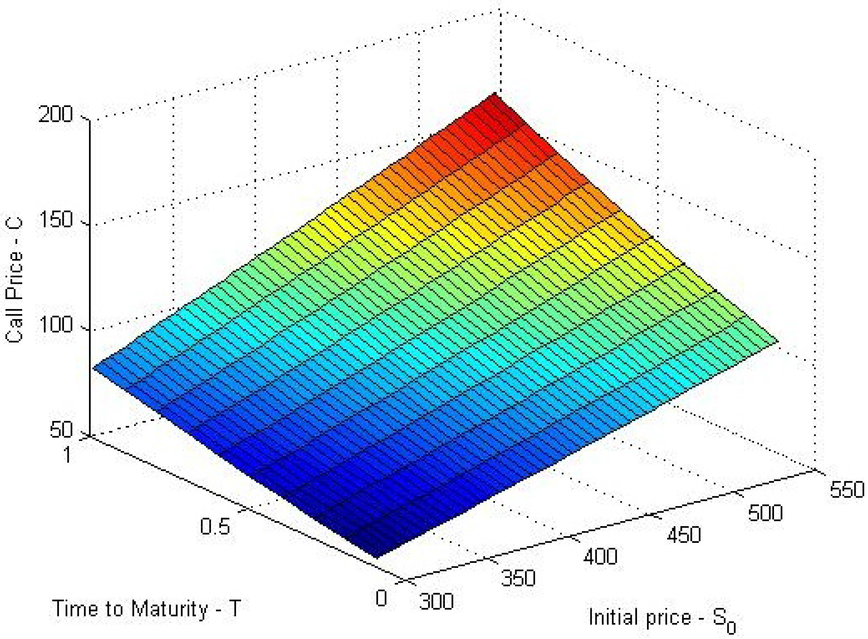
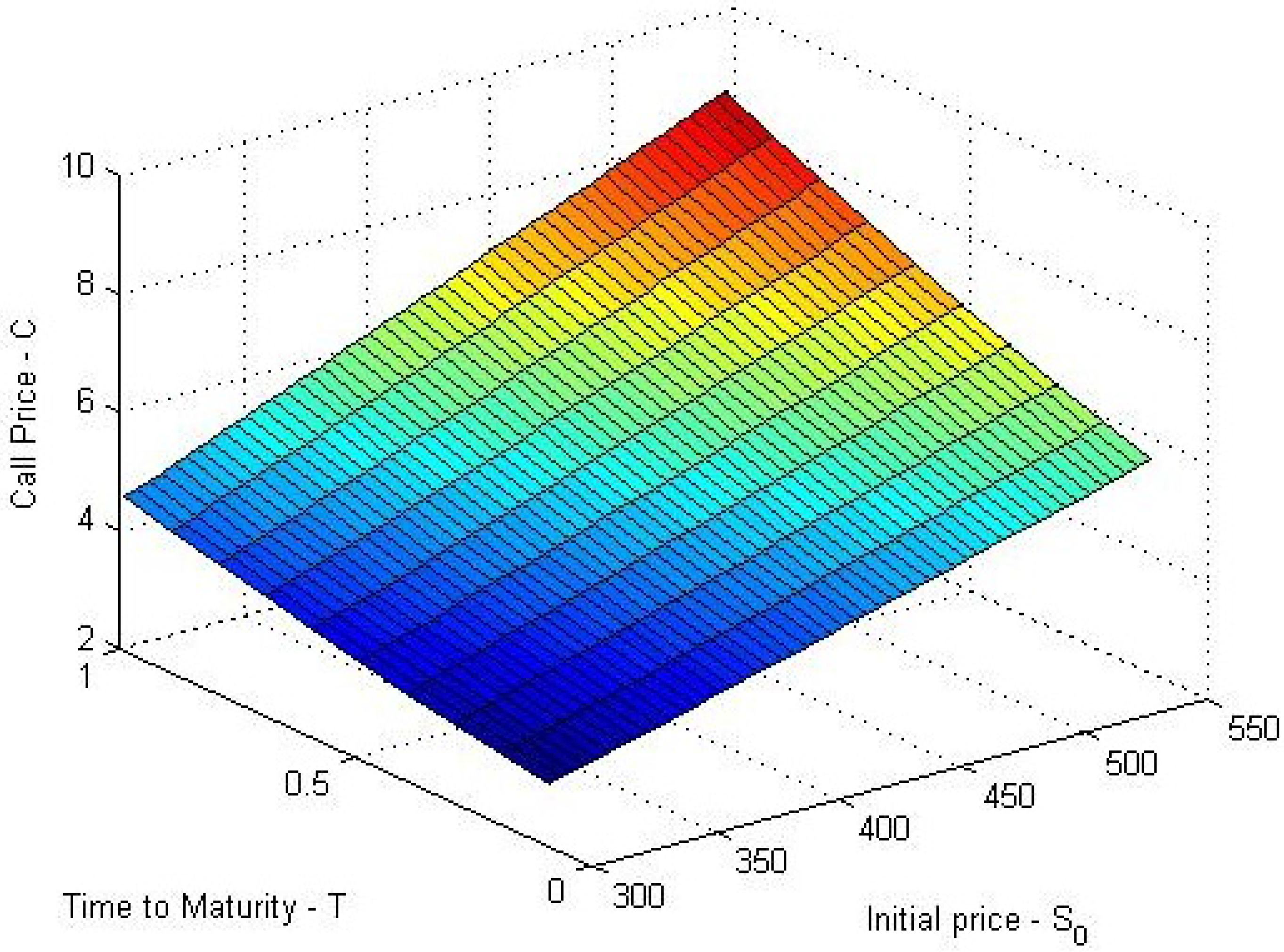
Algorithm 1 describes the procedure for computing the call price of the both Down-And-Out and Up-And-Out Barrier options. We have used above calibrated parameters to plot the call price plot against the Time-to-Maturity and Initial stock price for NIG, CGMY and Meixner processes in
Figure 1,
Figure 2,
Figure 3,
Figure 4,
Figure 5 and
Figure 6. This help us to understand how the call price changes with the change in stock price and maturity. The change of call price and sensitivities are also computed with the change of parameters such as volatility σ, Interest rate r, initial stock price
and Barrier B.
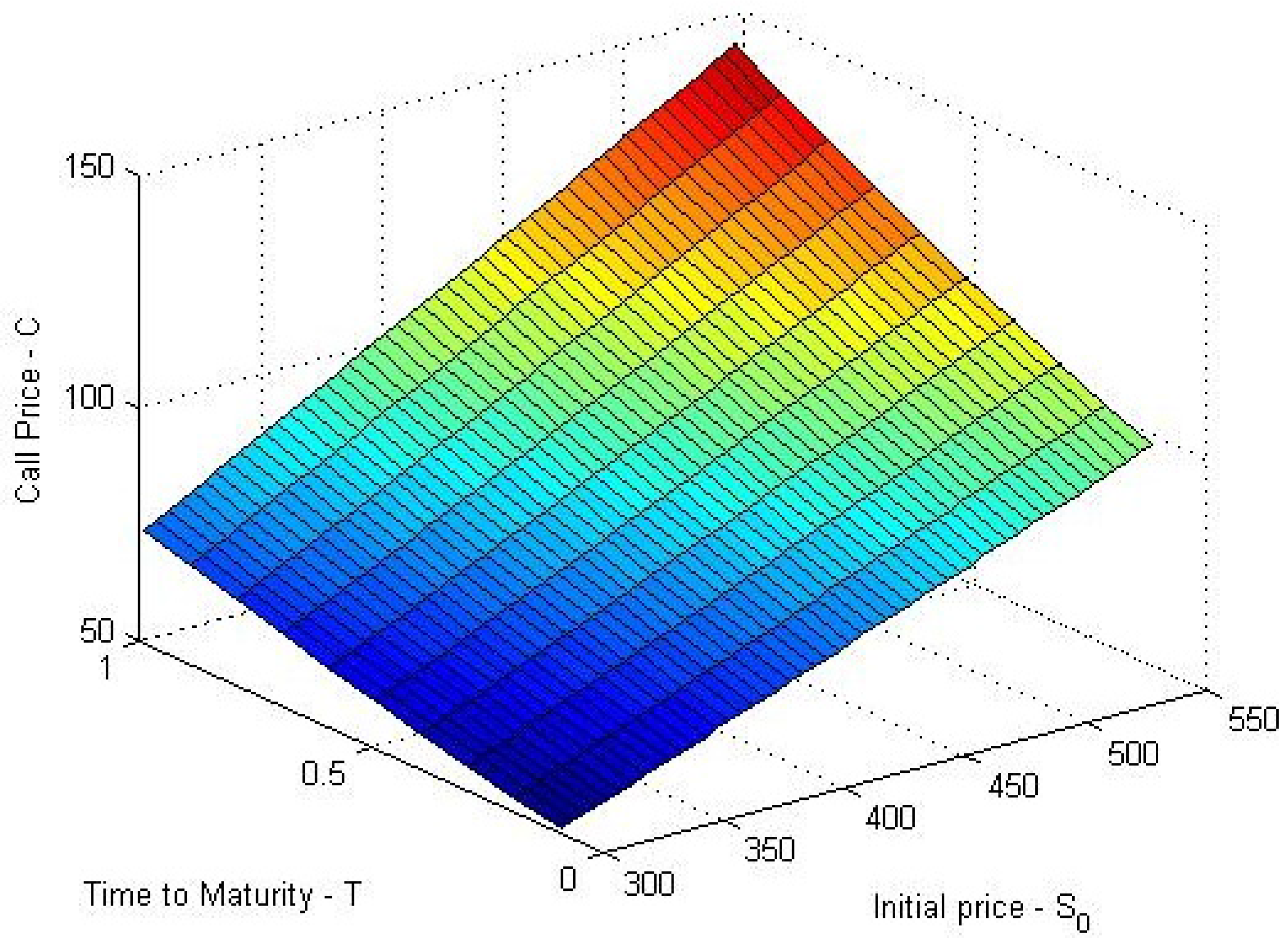
Figure 1.
Down-And-Out call with NIG process with Stock Price = 450, Strike price K = 150, Barrier B = 350, σ = 0.1812, r = 0.167 and Time to maturity T = 1.1.
Figure 1.
Down-And-Out call with NIG process with Stock Price = 450, Strike price K = 150, Barrier B = 350, σ = 0.1812, r = 0.167 and Time to maturity T = 1.1.
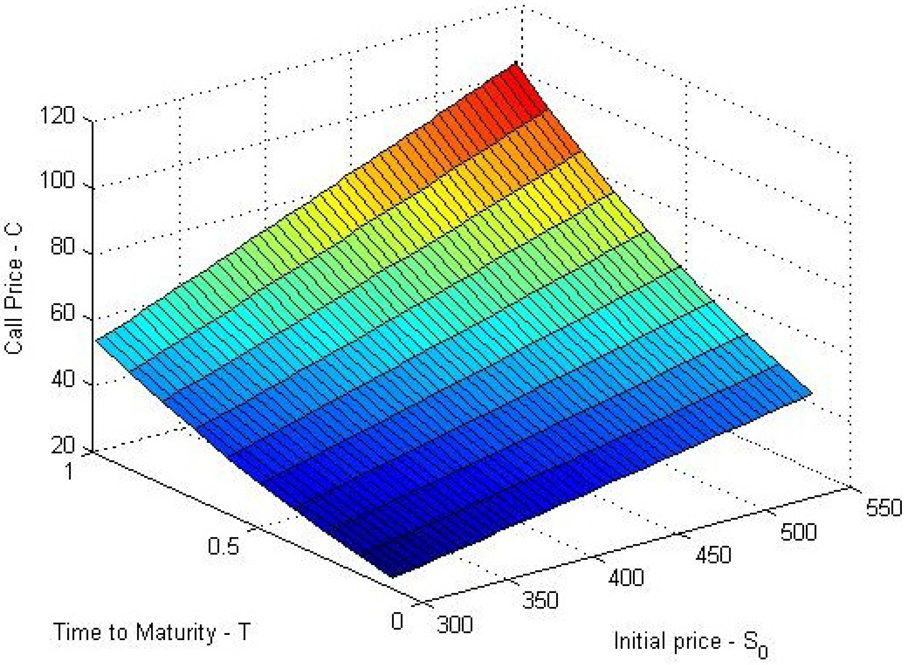
Figure 2.
Up-And-Out call with NIG (, , ) with Stock Price = 450, Strike price K = 150, Barrier B = 350, σ = 0.1812, r = 0.167 and Time to maturity T = 1.1.
Figure 2.
Up-And-Out call with NIG (, , ) with Stock Price = 450, Strike price K = 150, Barrier B = 350, σ = 0.1812, r = 0.167 and Time to maturity T = 1.1.
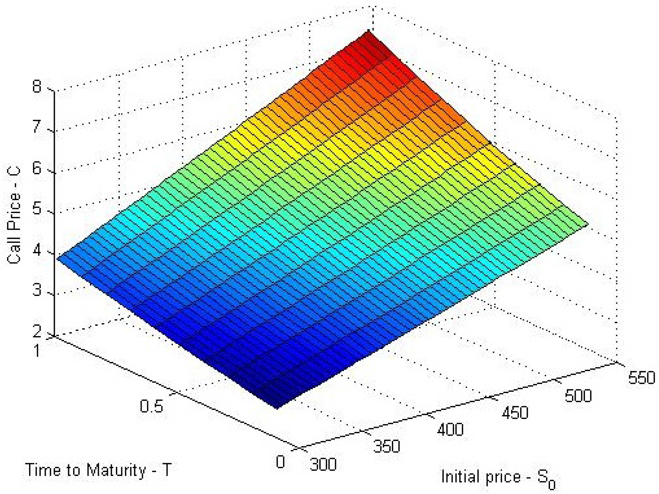
Figure 3.
Down-And-Out call with CGMY(, , , ) with Stock Price = 450, Strike price K = 150, Barrier B = 350, σ = 0.1812, r = 0.167 and Time to maturity T = 1.1.
Figure 3.
Down-And-Out call with CGMY(, , , ) with Stock Price = 450, Strike price K = 150, Barrier B = 350, σ = 0.1812, r = 0.167 and Time to maturity T = 1.1.
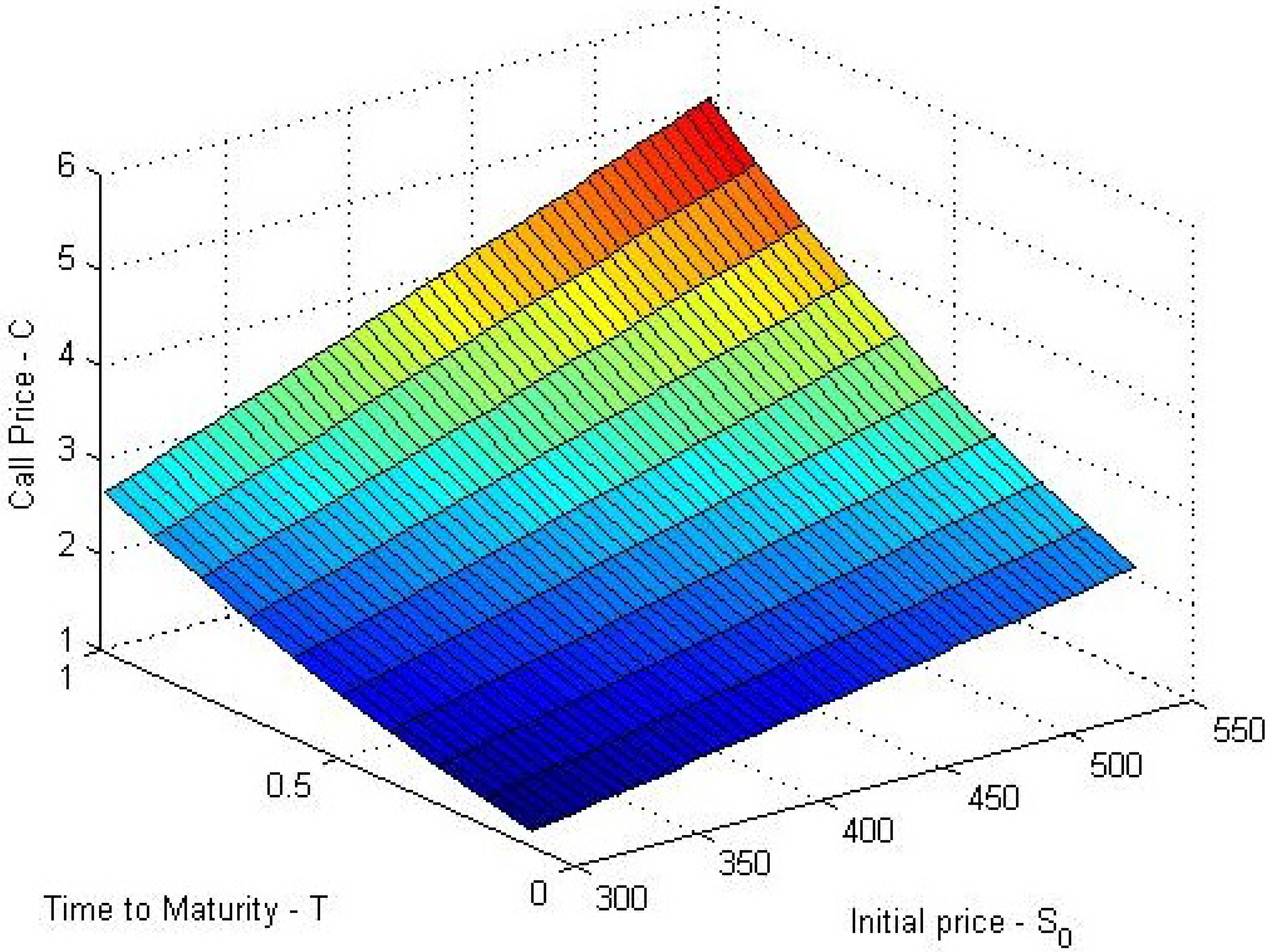
Figure 4.
Up-And-Out call with CGMY(, , , ) with Stock Price = 450, Strike price K = 150, Barrier B = 350, σ = 0.1812, r = 0.167 and Time to maturity T = 1.1.
Figure 4.
Up-And-Out call with CGMY(, , , ) with Stock Price = 450, Strike price K = 150, Barrier B = 350, σ = 0.1812, r = 0.167 and Time to maturity T = 1.1.
Figure 5.
Down-And-Out call with Meixner(, , ) with Stock Price = 450, Strike price K = 150, Barrier B = 350, σ = 0.1812, r = 0.167 and Time to maturity T = 1.1.
Figure 5.
Down-And-Out call with Meixner(, , ) with Stock Price = 450, Strike price K = 150, Barrier B = 350, σ = 0.1812, r = 0.167 and Time to maturity T = 1.1.
Figure 6.
Up-And-Out call with Meixner(, , ) with Stock Price = 450, Strike price K = 150, Barrier B = 350, σ = 0.1812, r = 0.167 and Time to maturity T = 1.1.
Figure 6.
Up-And-Out call with Meixner(, , ) with Stock Price = 450, Strike price K = 150, Barrier B = 350, σ = 0.1812, r = 0.167 and Time to maturity T = 1.1.
In
Table 1 we provide the calibration results for the given data set with three different processes (as Lévy density)- NIG, CGMY and Meixner. The Algorithm 1 used to compute the call price and sensitivities and result listed in
Table 2,
Table 3,
Table 4 and
Table 5. This result is also generated with the change of time-to-maturity, growth and volatility of the stock for different types of Lévy process.
Table 1.
Estimated parameters for Levy processes.
Table 1.
Estimated parameters for Levy processes.
| Model | | | Parameters | |
|---|
| NIG | | | | |
| CGMY | | | |
| Meixner | | | |
Table 2.
Change in Call Price with different types of Lévy Process.
Table 2.
Change in Call Price with different types of Lévy Process.
| t | r | σ | NIG (α, β, δ) Call | CGMY (C, G, M, Y) Call | Meixner (α, β, δ) Call |
|---|
| Down-Out | Up-Out | Down-Out | Up-Out | Down-Out | Up-Out |
|---|
| 1 | 0.167 | 0.5 | 8.8249 | 9.5132 | 8.4641 | 9.1207 | 8.8331 | 9.5222 |
| | 0.167 | 0.2 | 8.9626 | 9.6631 | 8.8112 | 9.4983 | 8.9689 | 9.6699 |
| 0.8 | 0.167 | 0.5 | 8.6620 | 9.3362 | 7.6423 | 8.2272 | 8.6863 | 9.3626 |
| | 0.167 | 0.2 | 9.0740 | 9.7843 | 8.6218 | 9.2924 | 9.0932 | 9.8052 |
| 0.5 | 0.167 | 0.5 | 8.4232 | 9.0767 | 6.5559 | 7.0477 | 8.4706 | 9.1282 |
| | 0.167 | 0.2 | 9.2436 | 9.9691 | 8.3454 | 8.9918 | 9.2827 | 10.0117 |
Table 3.
Call Price & Sensitivities change with Barrier.
Table 3.
Call Price & Sensitivities change with Barrier.
| Barrier (B) | Call | Delta | Gamma | Theta |
|---|
| Down-Out | Up-Out | Down-Out | Up-Out | Down-Out | Up-Out | Down-Out | Up-Out |
|---|
| 250 | 15.8960 | 3.4417 | 0.0410 | 0.0058 | 8.7909 | 1.9033 | −0.6604 | −0.1417 |
| 300 | 14.0080 | 5.3296 | 0.0374 | 0.0094 | 7.7468 | 2.9474 | −0.5825 | −0.2196 |
| 350 | 12.4266 | 6.9111 | 0.0342 | 0.0126 | 3.8220 | 6.8722 | −0.5172 | −0.2850 |
Table 4.
Change of Delta and Gamma over Stock price change.
Table 4.
Change of Delta and Gamma over Stock price change.
| S0 | NIG (α, β, δ) | CGMY (C, G, M, Y) | Meixner (α, β, δ) |
|---|
| Delta | Gamma | Delta | Gamma | Delta | Gamma |
|---|
| Down-Out | Up-Out | Down-Out | Up-Out | Down-Out | Up-Out | Down-Out | Up-Out | Down-Out | Up-Out | Down-Out | Up-Out |
|---|
| 350 | 0.03 | 0.01 | 6.87 | 3.82 | 0.02 | 0.01 | 4.97 | 4.61 | 0.02 | 0.01 | 5.53 | 5.13 |
| 400 | 0.03 | 0.01 | 9.09 | 5.05 | 0.02 | 0.01 | 6.58 | 6.09 | 0.03 | 0.01 | 7.32 | 6.78 |
| 450 | 0.04 | 0.01 | 11.64 | 6.45 | 0.03 | 0.01 | 8.42 | 7.80 | 0.03 | 0.02 | 9.38 | 8.67 |
Table 5.
Change of Theta over Time to expire.
Table 5.
Change of Theta over Time to expire.
| t | NIG (α, β, γ) Theta | CGMY (C, G, M, Y) Theta | Meixner (α, β, δ) Theta |
|---|
| Down-Out | Up-Out | Down-Out | Up-Out | Down-Out | Up-Out |
|---|
| 0.4 | −0.6851 | −0.3763 | 0.7374 | 0.6763 | −0.5246 | −0.4801 |
| 0.6 | −0.6753 | −0.3710 | 0.7536 | 0.6910 | −0.5175 | −0.4736 |
| 0.8 | −0.6655 | −0.3657 | 0.7702 | 0.7061 | −0.5104 | −0.4672 |
| 1.0 | −0.6560 | −0.3605 | 0.7871 | 0.7215 | −0.5034 | −0.4608 |
The Sensitivities like Delta, Gamma and Theta of the option with respect to initial stock price
and t will be denoted by
Using the above equations for sensitivities, we will check how the Call, Delta, Gamma & Theta changes with the change of Barrier for a specific type of Lévy process (in this case NIG) in the
Table 3.
The Call Price and Sensitivities (Delta, Gamma and Theta) computed (
Table 4 and
Table 5) for different types of Lévy process with its parameters.


