Article

From the Underdamped Generalized Elastic Model to the Single Particle Langevin Description

by
Alessandro Taloni
Center for Complexity and Biosystems and Department of Physics, University of Milano, Via Celoria 16, 20133 Milano, Italy
Mathematics 2017, 5(1), 3; https://doi.org/10.3390/math5010003
Submission received: 8 November 2016 / Revised: 12 December 2016 / Accepted: 19 December 2016 / Published: 6 January 2017
(This article belongs to the Special Issue Fractional Differential and Difference Equations)

Abstract

:
The generalized elastic model encompasses several linear stochastic models describing the dynamics of polymers, membranes, rough surfaces, and fluctuating interfaces. While usually defined in the overdamped case, in this paper we formally include the inertial term to account for the initial diffusive stages of the stochastic dynamics. We derive the generalized Langevin equation for a probe particle and we show that this equation reduces to the usual Langevin equation for Brownian motion, and to the fractional Langevin equation on the long-time limit.

1. Introduction

Linear stochastic systems describe a wealth of physical phenomena, ranging from polymer science to material science, where the elastic interactions inherent to the systems components are counterplayed by a friction dissipative force (damping). This dissipative force has the same microscopical nature of the randomly fluctuating force acting on each of the system components independently. The evolution equations of these many-body systems are encapsulated, in their most general formulations, in the so-called generalized elastic model (GEM).
The GEM has been firstly introduced in [1] through the following equation:
t h x , t = d d x Λ x x z x z h ( x , t ) + η x , t
The general formulation in (1) is given for the D-dimensional stochastic field h defined in the d-dimensional infinite space x . The zero-mean white noise η satisfies the fluctuation-dissipation (FD) relation, i.e.:
η j x , t η k x , t = 2 k B T Λ x x δ j k δ ( t t )
( j , k [ 1 , D ] ), where Λ r = 1 / r α corresponds to the hydrodynamic friction kernel whose Fourier transform is:
Λ q = ( 4 π ) d / 2 γ 2 α Γ ( d α ) / 2 Γ α / 2 q α d = A q α d
if d 1 2 < α < d . Notice that in the previous equation γ represents a friction constant and Γ ( ) stands for the Gamma function [2]. The fractional derivative z / x z , defined via its Fourier transform by [3]:
F q z x z q z
has another common definition given in term of the Laplacian Δ as z x z : = Δ z / 2 [4]. The GEM (1) accounts for the dynamics of polymers [5,6,7,8,9], elastic chains [10,11,12], membranes [6,13,14,15,16,17] and rough surfaces [18,19,20,21,22], among others. It also reproduces the anomalous diffusive behavior of systems such as crack propagation [23] and contact line of a liquid meniscus [24]. Each one of the above-mentioned physical systems corresponds to a given set of the parameters defining the GEM (1), namely z , α and d, with α = d in the case of Λ r = δ r γ ( A = c o n s t in (3)). The latter indeed corresponds to the case of locally hydrodynamic systems [25,26], i.e., those systems where hydrodynamic interactions can be considered negligibles or entirely screened out. In the present article, for the sake of clarity and not to burden the notation, we will deal with this class of systems, bearing in mind that the whole framework can be easily extended to systems with long ranged hydrodynamic interactions.
In Refs [1,25] it was derived the fractional Langevin equation (FLE) governing the dynamics of a tagged point (hereafter named probe or tracer without distinction) on the GEM (1). The probe can represent a spot on a membrane surface, or a tracer particle among those composing a single file system, or a tagged monomer in polymeric chains. This equation has the same structure as of an overdamped Langevin equation, but its time derivative is replaced by a Riemann-Liouville pseudodifferential operator [4,27]:
K + D t β h x , t = ζ x , t
with:
D t β ϕ ( t ) = 1 Γ 1 β d d t t d t 1 t t β ϕ t . 0 < β < 1
Although the GEM (1) is defined neglecting inertial effects, it is instructive to consider also these while providing a comprehensive treatment. Our pricipal aim is to provide the derivation of the equation for a tracer only, disregarding the rest of the system. In other words we plan to derive the equivalent of the FLE (5) for systems where inertial effects cannot be discarded. This equation should properly reproduce any stochastic regime attained by the tagged particle, reducing to the FLE for long times.

2. Underdamped Generalized Elastic Model

Let us start by considering the GEM, including the inertial effects, i.e., the underdamped generalized elastic model (UGEM):
2 t 2 h x , t + γ t h x , t k z z x z h ( x , t ) = ξ x , t
where the noise term, appearing on the RHS, satisfies the FD relation:
ξ j x , t ξ k x , t = 2 k B T γ δ j k δ x x δ ( t t )
with ξ j x , t = 0 , j . The constant k z on the LHS has the dimensions of [ l ] z [ t ] 2 . It is straightforwardly proven that Equation (7) reduces to (1) (where hydrodynamic effects are disregarded) once the inertial term is neglected ( t ) and the white noise is taken η x , t = ξ x , t γ . We recall that no retarded viscoelastic effects are considered hereafter, i.e., the friction term in the LHS of Equation (7) is only of the kind γ t h x , t . Although the insertion of a retarded (fractional) memory kernel indeed does not not present any mathematical difficulty, the material viscoelastic properties are disregarded in our analysis and the frictional force is uniquely determined by the external noise source.
First, in analogy to the overdamped case [1,25], let us consider just one component of the vector field h , h = h j . Second, we introduce the Fourier transform of a function g x , t as:
g q , ω = + d x + d t g x , t e i q · x ω t
and its inverse as:
g x , t = + d q ( 2 π ) d + d ω 2 π g q , ω e i q · x ω t
Hence, the FD relationship (8) reads in the Fourier space:
ξ j q , ω ξ k q , ω = 2 k B T γ ( 2 π ) d + 1 δ j k δ q + q δ ( ω ω )
Moreover, taking the Fourier transform on both sides of the Equation (7), the solution of the UGEM is easily found to be:
h q , ω = ξ q , ω ω 2 i ω γ + k z q z
owing to the Defintion (4).
We seek the evolution equation for the stochastic field h x , t placed in the position x at time t. Our treatment traces substantially that developed in Refs [1,25,26,28,29]. We start by multiplying both sides of Equation (12) by f ( ω ) , which is a complex function of a real variable:
f ( ω ) h q , ω = f ( ω ) ξ q , ω ω 2 i ω γ + k z q z
Hence we define two quantities: the retarded friction kernel γ ˜ ( t ) [30] and the noise-propagator [25,26,29,31] Φ x , t . They are defined in the Fourier space through the relations:
γ ˜ ( ω ) = f ( ω ) i ω
and:
Φ q , ω = f ( ω ) ω 2 i ω γ + k z q z
They both represent the effect of the whole system on the dynamics of a single probe placed at the point x . The friction kernel embodies the reterded memory effects. The noise-propagator has the same structure of a Green function for the white noise term, i.e., it carries the thermal perturbation between two points of the system, in a certain lapse of time. Their action on the probe stochastic dynamics becomes clear after recasting the Equation (13) using Definitions (14) and (15):
γ ˜ ( ω ) ( i ω ) h q , ω = Φ q , ω ξ q , ω
Now, let us perform the inverse Fourier transform in time and space of the previous equation:
d t γ ˜ ( t t ) t h x , t = d x d t Φ x x , t t ξ x , t
and define the noise on the RHS as:
ζ x , t = d x d t Φ x x , t t ξ x , t
It appears clear that the noise ζ x , t results from the convolution of the thermal contributions on the points x , to the point of interest x (the probe). These contributions are weighted by the noise-propagator Φ x x , t t , which transmits the perturbation taking place on the point x at time t to the point x at the time t. It is also clear that the noise ζ x , t is Gaussian and correlated in space and in time. By the insertion of Equation (18) into Equation (17) one gets the sought equation for the single probe:
d t γ ˜ ( t t ) t h x , t = ζ x , t
which is the typical form of a generalized Langevin Equation [32,33,34].
To complete the derivation we need to enforce the generalized FD relationship between the damping kernel and the colored Gaussian noise, i.e.:
ζ x , t ζ x , t = k B T γ ˜ ( t t )
Taking the Fourier transform in time, the following relation is derived directly from Equation (20):
ζ x , ω ζ x , ω = 4 π k B T e γ ˜ ( ω ) δ ( ω + ω )
In view of the expressions (14), (15) and (18), the requirement (21) entails the constitutive equation for the complex function f ( ω ) . In the next subsection we will derive the analytical form of f ( ω ) , satisfying the FD condition (21).

2.1. Generalized FD Relationship

The LHS of (21) can be calculated explicitey:
ζ x , ω ζ x , ω = d x 1 d x 2 Φ x x 1 , ω Φ x x 2 , ω ξ x 1 , ω ξ x 2 , ω
In view of Equation (11), the Fourier transform in time of the noise correlation function (8) is ξ x 1 , ω ξ x 2 , t = 4 k B T γ π δ x 1 x 2 δ ( ω + ω ) . Plugging this expression into Equation (22) yields:
ζ x , ω ζ x , ω = 4 k B T γ π d x 1 Φ x x 1 , ω Φ x x 1 , ω
Now, the Formulas (10) and (15) require that:
ζ x , ω ζ x , ω = 4 k B T γ π d x 1 e i q 1 + q 2 · x 1 d q 1 ( 2 π ) d d q 2 ( 2 π ) d f ( ω ) f ( ω ) e i q 1 + q 2 · x ω 2 i ω γ + k z q 1 z ω 2 + i ω γ + k z q 2 z
Recalling one of the definitions of the Dirac’s delta function, namely δ q = d x ( 2 π ) d e i q · x , we get the expression:
ζ x , ω ζ x , ω = 4 π k B T γ δ ω + ω d q 1 ( 2 π ) d f ( ω ) f ( ω ) ω 2 γ 2 + ω 4 2 ω 2 k z q 1 z + k z 2 q 1 2 z
Since the integrand function is solely depending on the magnitude of the vector q 1 , we integrate out the angular dependence in the previous integral obtaining:
ζ x , ω ζ x , ω = 2 3 d π 1 d / 2 k B T γ Γ d 2 δ ω + ω f ( ω ) f ( ω ) ω 2 γ 2 + ω 4 0 d q 1 q 1 d 1 1 2 k z ω 2 q 1 z ω 2 γ 2 + ω 4 + k z 2 q 1 2 z ω 2 γ 2 + ω 4
By the following change of variable y = q 1 ω 2 γ 2 + ω 4 1 / ( 2 z ) , we can study the integral:
I ( ω ) = ω 2 γ 2 + ω 4 d 2 z 0 d y y d 1 1 2 ω 2 ω 2 γ 2 + ω 4 1 / 2 k z y z + k z y z 2
Hence, we further transform u = k z y z to obtain:
I ( ω ) = ω 2 γ 2 + ω 4 d 2 z z k z d z 0 d u u d / z 1 1 | ω | γ 2 + ω 2 1 / 2 u + u 2
Finally, this integral can be solved explicitely [35] and we find:
I ( ω ) = π z k z d z sin d π z | ω | d z γ 2 + ω 2 d 2 z sin z d z cos 1 | ω | γ 2 + ω 2 1 / 2 sin cos 1 | ω | γ 2 + ω 2 1 / 2
Let us now introduce the function:
μ ω = cos 1 | ω | γ 2 + ω 2 1 / 2
which is shown in Figure 1 for different values of the dampiung coefficient γ. From Equation (30) it appears clear that this function, which is a real function, appears to be universal and independent of the values of z and d.
We can expand:
sin z d z μ ω = sin μ ω cos d z μ ω + | ω | γ 2 + ω 2 1 / 2 sin d z μ ω
and, recalling that:
sin cos 1 | ω | γ 2 + ω 2 1 / 2 = γ γ 2 ω 2
we can recast the integral (29) in the following form:
I ( ω ) = π z k z d z sin d π z | ω | d z γ 2 + ω 2 d 2 z cos d z μ ω + | ω | γ sin d z μ ω
that can be inserted in the noise correlation expression (26) yielding:
ζ x , ω ζ x , ω = 2 3 d π 2 d / 2 k B T γ Γ d 2 z k z d z sin d π z δ ω + ω | ω | d / z 2 γ 2 + ω 2 d 2 z 1 f ( ω ) f ( ω ) cos d z μ ω + | ω | γ sin d z μ ω
Now, from the defintion (20) we know that the noise ζ x , t is stationary, therefore thanks to the Wiener-Kintchine theorem [36] the Fourier transform of its correlation function must be real and proportional to its power spectrum. This entails that:
f ( ω ) = f * ( ω )
and in turns f ( ω ) f ( ω ) = f ( ω ) 2 . Once substituted into Equation (32), the previous condition gives the final expression of the RHS of the FD theorem (21):
ζ x , ω ζ x , ω = 2 3 d π 2 d / 2 k B T γ Γ d 2 z k z d z sin d π z δ ω + ω | ω | d / z 2 γ 2 + ω 2 d 2 z 1 f ( ω ) 2 cos d z μ ω + | ω | γ sin d z μ ω
The LHS of Equation (21) is easily calculated from the definition of the damping kernel (14), i.e., e γ ˜ ( ω ) = m f ( ω ) ω ω 2 thus yielding the constraint that the function f ( ω ) must fulfill:
2 1 d π 1 d / 2 γ Γ d 2 z k z d z sin d π z | ω | d / z γ 2 + ω 2 d 2 z 1 cos d z μ ω + | ω | γ sin d z μ ω = m f ( ω ) ω f ( ω ) 2
Let us take:
f ( ω ) = ρ ( ω ) e i ϕ ( ω )
where ρ ( ω ) and ϕ ( ω ) are chosen to be two real functions of real variable. As a consequence, the requirement (33) provides that the radial part of f ( ω ) is even under time reversal symmetry ρ ( ω ) = ρ ( ω ) , and the phase is odd ϕ ( ω ) = ϕ ( ω ) . When substituted into Equation (35), the definition (36) gives the relation between the radial part ( ρ ( ω ) ) and its phase ( ϕ ( ω ) ), i.e.:
2 1 d π 1 d / 2 γ Γ d 2 z k z d z sin d π z | ω | d / z γ 2 + ω 2 d 2 z 1 cos d z μ ω + | ω | γ sin d z μ ω = sin ϕ ( ω ) ω ρ ( ω )
Thanks to the symmetries of ρ ( ω ) and ϕ ( ω ) we finally obtain:
2 1 d π 1 d / 2 γ Γ d 2 z k z d z sin d π z | ω | d / z 1 γ 2 + ω 2 d 2 z 1 cos d z μ ω + | ω | γ sin d z μ ω = sin ϕ ( ω ) ρ ( ω )
Consider the following solution:
ρ ( ω ) = Γ ( d / 2 ) z k z d z sin d π z sin z d z μ ω | ω | z d z 2 1 d π 1 d / 2 γ γ 2 + ω 2 d 2 z 1 cos d z μ ω + | ω | γ sin d z μ ω ϕ ( ω ) = z d z s i g n ( ω ) μ ( ω )
where the function s i g n ( ω ) is = 1 for ω > 0 and = 1 when ω < 0 . It is straightforward to prove that the expression (39) satisfies the Equation (37). Both functions are shown in Figure 2 taking d = 1 , γ = 2 and several values of z.

2.2. Limiting Behaviours

The Equations (36) and (39) constitute the central results of this paper. As a matter of fact, once plugged into the damping kernel expression (14) and into the noise propagator (15), they assure that the probe stochastic dynamics is described by a generalized Langevin equation such that Equation (19), when the noise on the LHS satisfies the generalized FD relation (20) at any time. That means that the different regimes undergone by a probe or a tracer is exactly reproduced by Equation (19). This is analyticaly addressed in the following.
  • Short time limit: t 0 , i.e., ω 2 k z | q | z , | q | .
    This situation refer to the case where the fractional interactions among the system components are not yet sufficiently strong to affect the dynamics of the tracer. In this case the solution (12) takes the following form:
    h q , ω ξ q , ω ω 2 i ω γ
    which is the solution of an underdamped classical Langevin equation of a Brownian particle:
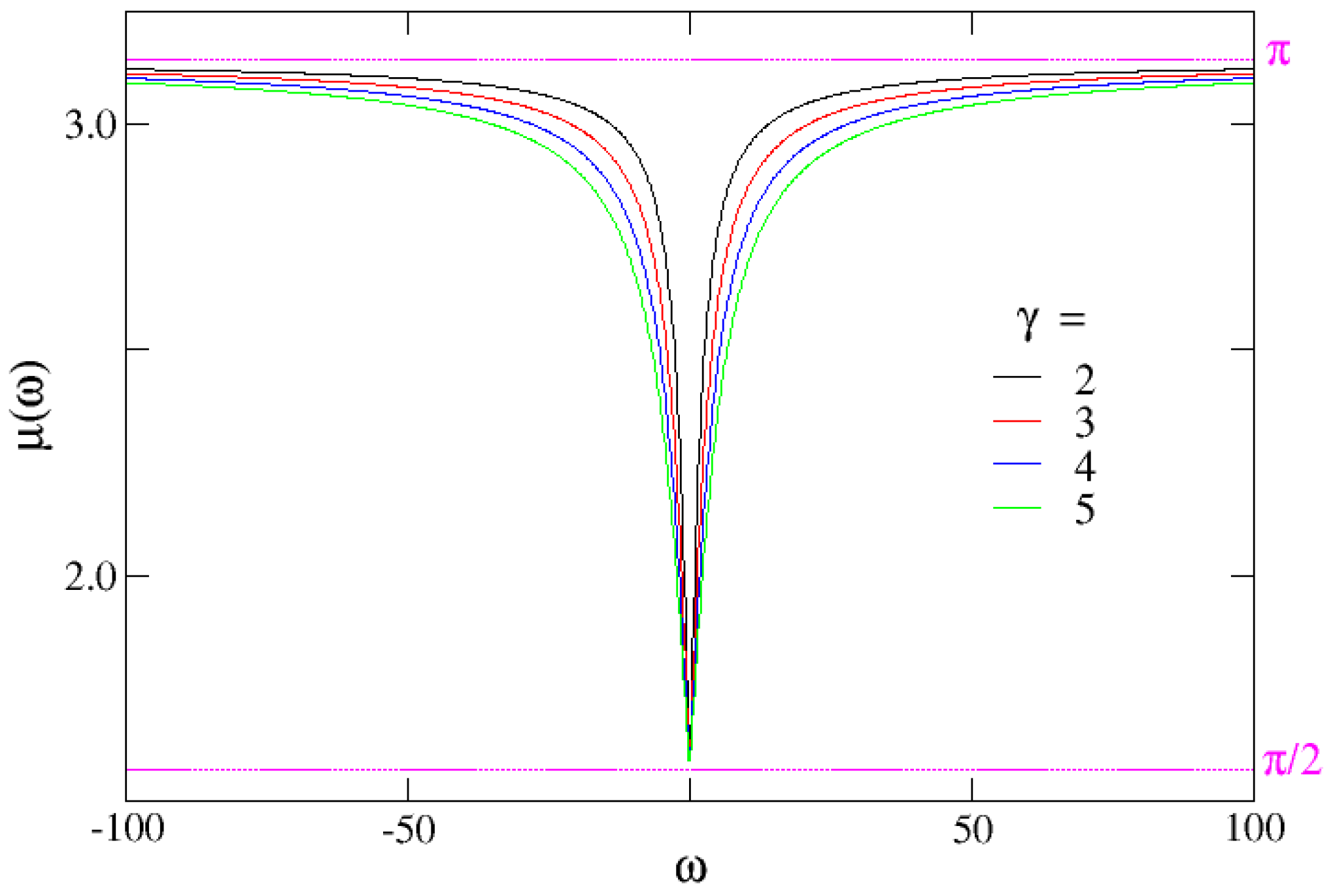
    2 t 2 h x , t + γ t h x , t = ξ x , t
  • Long time limit: t , i.e., ω 2 k z | q | z , | q | .
    In this case the Fourier solution of the UGEM in Equation (12) can be written neglecting the inertia of the system:
    h q , ω = ξ q , ω i ω γ + k z q z
    This limit entails that μ ( ω ) π 2 as it can be seen from the expression (30) and Figure 1. Consequently the phase ϕ ( ω ) tends to a constant: ϕ ( ω ) ( z d ) π 2 d s i g n ( ω ) . Hence, from expression (36), after straightforward algebraic passages one obtains:
    f ( ω ) = Γ ( d / 2 ) z k z d z sin d π z e i π 2 s i g n ( ω ) | ω | z d z 2 1 d π 1 d / 2 γ d z z
    which can be casted in the final form:
    f ( ω ) = Γ ( d / 2 ) z k z d z sin d π z i ω z d z 2 1 d π 1 d / 2 γ d z z
    Now, defining the constant prefactor [1,26]:
    K + = Γ ( d / 2 ) z k z d z sin d π z 2 1 d π 1 d / 2 γ d z z
    the Equation (16) transforms to:
    K + i ω z d z h q , ω = Φ q , ω ξ q , ω
    where the Fourier transform of the noise propagator is:
    Φ q , ω = K + i ω z d z i ω γ + k z q z
    from Equation (15). Recalling that ( i ω ) β represents the Fourier transform of the the left side Riemann-Liouville derivative (6) with lower bound [4,27,29,31] and that is equivalent to the Caputo [37] derivative [27], i.e.:
    d β d t β X ( t ) = 1 Γ ( 1 β ) t d t X ˙ ( t ) ( t t ) β 0 < β < 1
    we can express in space-time domain the expression (45) recovering the FLE (5):
    K + D t β h x , t = ζ x , t
    The fractional Brownian noise on the RHS is defined by the Equation (18) via Equation (46).
In summary we have demonstrated that the Equation (19), with the definition of the damping kernel:
γ ( t ) = d ω 2 π Γ ( d / 2 ) z k z d z sin d π z sin z d z μ ω | ω | z d z e i ω t + ( z d ) z s i g n ( ω ) μ ( ω ) 2 1 d π 1 d / 2 γ γ 2 + ω 2 d 2 z 1 ( i ω ) cos d z μ ω + | ω | γ sin d z μ ω
and the noise in (18), with the noise propagator introduced as:
Φ ( x , t ) = + d q ( 2 π ) d + d ω 2 π Γ ( d / 2 ) z k z d z sin d π z sin z d z μ ω | ω | z d z e i q · x ω t ( z d ) z s i g n ( ω ) μ ( ω ) 2 1 d π 1 d / 2 γ γ 2 + ω 2 d 2 z 1 ω 2 i ω γ + k z q z cos d z μ ω + | ω | γ sin d z μ ω
constitutes the general stochastic equation ruling the motion of a tracer (the function μ ( ω ) being defined in (30)). Remarkably this equation interpolates between the normal diffusive behaviour at short times (41), and the FLE (42) at long times. As such, this equation can reproduce the three diffusional regimes of a tracer, i.e., ballistic δ 2 h ( x , t ) t 2 for 0 t 1 γ , linear δ 2 h ( x , t ) t for 1 γ t a z 2 k z , and subdiffusive δ 2 h ( x , t ) t z d d for t a z 2 k z , where a is a characteristic length scale of the system.

3. Conclusions

In this article we have rogorously derived an equation for the stocahstic motion of a tracer particle in a underdamped generalized elastic model (7). This equation takes the form of a generalized Langevin equation with the damping kernel and the thermal noise satisfying the FD theorem at any time. It is not the first time that a form of GLE is introduced to account for the different diffusional stages of a tracer in a linear interacting system. Indeed, in a single file system, the following stochastic equation was proposed for the tagged particle motion [30]:
d 2 h ( x , t ) d t 2 = 0 t γ t t d h ( x , t ) d t d t + ξ ˜ ( x , t )
The tracer dynamics indeed is ballistic for t 1 γ , diffusive for intermediate times 1 γ t τ d , and finally subdiffusice ( δ 2 h ( x , t ) t ) for t τ d . The generalized damping kernel interpolates between the two asymptotic behaviors:
γ ˜ ( t ) = 2 γ δ ( t ) + 1 π τ d t
This equation was proven extremely useful for reproducing any single particle observable, which indeed exhibites different time behaviors corresponding to the specific time scales. However, Equation (51) was just postulated in [30] and not derived from the microscopic dynamics of the whole system, as it has been performed in the present article. The analytical derivation presented here, can be straightforwardly extended to any underdamped linearly interacting system belonging to the UGEM universality class . Moreover, it appears clear as the friction and the noise terms are not time invariant. They change according to the nature of the interactions that the tracer experiences in its motion: the noise is delta correlated in time and the damping constant, as the tracer dynamics if fluid-driven, but it develops long-ranged tails when the elastic interactions with the rest of the system become dominant. Correspondingly, the damping is characterized by persistent memory effects, expressed in a compact mathematical formulation by the fractional derivative in time.

Acknowledgments

The author acknowledges the European Research Council through the Advanced Grant No. 291002 SIZEFFECTS.

Conflicts of Interest

The author declares no conflict of interest.

Abbreviations

The following abbreviations are used in this manuscript:
GEMGeneralized elastic model
FDFluctuation-dissipation
RHSRight-hand side
LHSLeft-hand side
GLEGeneralized Langevin equation
FLEFractional Langevin equation
UGEMUnderdamped generalized elastic model

References

  1. Taloni, A.; Chechkin, A.; Klafter, J. Generalized elastic model yields a fractional Langevin equation description. Phys. Rev. Lett. 2010, 104, 160602. [Google Scholar] [CrossRef] [PubMed]
  2. Abramowitz, M.; Stegun, I.A. Handbook of Mathematical Functions: With Formulas, Graphs, and Mathematical Tables CONFIRMED; Courier Corporation: North Chelmsford, MA, USA, 1964; Volume 55. [Google Scholar]
  3. Saichev, A.I.; Zaslavsky, G.M. Fractional kinetic equations: Solutions and applications. Chaos Interdiscip. J. Nonlinear Sci. 1997, 7, 753–764. [Google Scholar] [CrossRef] [PubMed]
  4. Samko, S.G.; Kilbas, A.A.; Marichev, O.I. Fractional Integrals and Derivatives. Theory and Applications; Gordon and Breach: Yverdon, Switzerland, 1993. [Google Scholar]
  5. Doi, M.; Edwards, S.F. The Theory of Polymer Dynamics; Oxford University Press: Oxford, UK, 1988; Volume 73. [Google Scholar]
  6. Granek, R. From semi-flexible polymers to membranes: Anomalous diffusion and reptation. J. Phys. II 1997, 7, 1761–1788. [Google Scholar] [CrossRef]
  7. Farge, E.; Maggs, A.C. Dynamic scattering from semiflexible polymers. Macromolecules 1993, 26, 5041–5044. [Google Scholar] [CrossRef]
  8. Caspi, A.; Elbaum, M.; Granek, R.; Lachish, A.; Zbaida, D. Semiflexible polymer network: A view from inside. Phys. Rev. Lett. 1998, 80, 1106. [Google Scholar] [CrossRef]
  9. Amblard, F.; Maggs, A.C.; Yurke, B.; Pargellis, A.N.; Leibler, S. Subdiffusion and anomalous local viscoelasticity in actin networks. Phys. Rev. Lett. 1996, 77, 4470. [Google Scholar] [CrossRef] [PubMed]
  10. Edwards, S.F.; Wilkinson, D. The surface statistics of a granular aggregate. In Proceedings of the Royal Society of London A: Mathematical, Physical and Engineering Sciences; The Royal Society: London, UK, 1982; Volume 381, pp. 17–31. [Google Scholar]
  11. Rouse, P.E., Jr. A theory of the linear viscoelastic properties of dilute solutions of coiling polymers. J. Chem. Phys. 1953, 21, 1272–1280. [Google Scholar] [CrossRef]
  12. Zimm, B.H. Dynamics of polymer molecules in dilute solution: Viscoelasticity, flow birefringence and dielectric loss. J. Chem. Phys. 1956, 24, 269–278. [Google Scholar] [CrossRef]
  13. Freyssingeas, É.; Roux, D.; Nallet, F. Quasi-Elastic Light Scattering Study of Highly Swollen Lamellar and Sponge. J. Phys. II 1997, 7, 913–929. [Google Scholar] [CrossRef]
  14. Helfer, E.; Harlepp, S.; Bourdieu, L.; Robert, J.; MacKintosh, F.; Chatenay, D. Microrheology of biopolymer-membrane complexes. Phys. Rev. Lett. 2000, 85, 457. [Google Scholar] [CrossRef] [PubMed]
  15. Granek, R.; Klafter, J. Anomalous motion of membranes under a localized external potential. EPL (Europhys. Lett.) 2001, 56, 15. [Google Scholar] [CrossRef]
  16. Zilman, A.G.; Granek, R. Membrane dynamics and structure factor. Chem. Phys. 2002, 284, 195–204. [Google Scholar] [CrossRef]
  17. Zilman, A.; Granek, R. Dynamics of fractal sol-gel polymeric clusters. Phys. Rev. E 1998, 58, R2725. [Google Scholar] [CrossRef]
  18. Majumdar, S.N.; Bray, A.J. Spatial persistence of fluctuating interfaces. Phys. Rev. Lett. 2001, 86, 3700. [Google Scholar] [CrossRef] [PubMed]
  19. Majaniemi, S.; Ala-Nissila, T.; Krug, J. Kinetic roughening of surfaces: Derivation, solution, and application of linear growth equations. Phys. Rev. B 1996, 53, 8071. [Google Scholar] [CrossRef]
  20. Searson, P.; Li, R.; Sieradzki, K. Surface diffusion in the solid-on-solid model. Phys. Rev. Lett. 1995, 74, 1395. [Google Scholar] [CrossRef] [PubMed]
  21. Krug, J. Origins of scale invariance in growth processes. Adv. Phys. 1997, 46, 139–282. [Google Scholar] [CrossRef]
  22. Toroczkai, Z.; Williams, E.D. Nanoscale fluctuations at solid surfaces. Phys. Today 1999, 52, 24–28. [Google Scholar] [CrossRef]
  23. Gao, H.; Rice, J.R. A first-order perturbation analysis of crack trapping by arrays of obstacles. J. Appl. Mech. 1989, 56, 828–836. [Google Scholar] [CrossRef]
  24. Joanny, J.; De Gennes, P.G. A model for contact angle hysteresis. J. Chem. Phys. 1984, 81, 552–562. [Google Scholar] [CrossRef]
  25. Taloni, A.; Chechkin, A.; Klafter, J. Unusual response to a localized perturbation in a generalized elastic model. Phys. Rev. E 2011, 84, 021101. [Google Scholar] [CrossRef] [PubMed]
  26. Taloni, A.; Chechkin, A.; Klafter, J. Correlations in a generalized elastic model: Fractional Langevin equation approach. Phys. Rev. E 2010, 82, 061104. [Google Scholar] [CrossRef] [PubMed]
  27. Podlubny, I. Fractional Differential Equations: An Introduction to Fractional Derivatives, Fractional Differential Equations, to Methods of Their Solution and Some of Their Applications; Academic Press: Cambridge, MA, USA, 1998; Volume 198. [Google Scholar]
  28. Taloni, A.; Chechkin, A.; Klafter, J. Generalized elastic model: Thermal vs. non-thermal initial conditions—Universal scaling, roughening, ageing and ergodicity. EPL (Europhys. Lett.) 2012, 97, 30001. [Google Scholar] [CrossRef]
  29. Taloni, A.; Chechkin, A.; Klafter, J. Generalized elastic model: Fractional Langevin description, fluctuation relation and linear response. Math. Model. Nat. Phenom. 2013, 8, 127–143. [Google Scholar] [CrossRef]
  30. Taloni, A.; Lomholt, M.A. Langevin formulation for single-file diffusion. Phys. Rev. E 2008, 78, 051116. [Google Scholar] [CrossRef] [PubMed]
  31. Taloni, A. Kubo Fluctuation Relations in the Generalized Elastic Model. Adv. Math. Phys. 2016, 2016, 7502472. [Google Scholar] [CrossRef]
  32. Mori, H. A quantum-statistical theory of transport processes. J. Phys. Soc. Jpn. 1956, 11, 1029–1044. [Google Scholar] [CrossRef]
  33. Mori, H. A continued-fraction representation of the time-correlation functions. Prog. Theor. Phys. 1965, 34, 399–416. [Google Scholar] [CrossRef]
  34. Mori, H. Transport, collective motion, and Brownian motion. Prog. Theor. Phys. 1965, 33, 423–455. [Google Scholar] [CrossRef]
  35. Gradshtein, I.S.; Ryzhik, I.M. Tables of Integrals, Sums, Series, and Products; Academic Press: Cambridge, MA, USA, 1971. [Google Scholar]
  36. Wiener, N. Extrapolation, Interpolation, and Smoothing of Stationary Time Series; MIT Press Cambridge: Cambridge, MA, USA, 1949; Volume 2. [Google Scholar]
  37. Caputo, M. Linear models of dissipation whose Q is almost frequency independent—II. Geophys. J. Int. 1967, 13, 529–539. [Google Scholar] [CrossRef]
Figure 1. μ ( ω ) . The function defined in (30) for several value of the damping constant γ. Notice as this function is universal, i.e., is independent of the fractional exponent z and of the dimension of the substrate d. Notice the limit in the short and long time limit, π and π 2 respectively.
Mathematics 05 00003 g001
Figure 2. ρ ( ω ) and ϕ ( ω ) . Radial part (a) and phase (b) of the complex function f ( ω ) as defined by Equation (36). Notice that ρ ( ω ) and ϕ ( ω ) are real functions of a real variable.
Mathematics 05 00003 g002

