Scaling Laws in the Fine-Scale Structure of Range Margins

Department Plant Taxonomy, Ecology and Theoretical Biology, Loránd Eötvös University, Budapest H-1117, Hungary
Mathematics 2018, 6(12), 315; https://doi.org/10.3390/math6120315
Submission received: 5 November 2018
/
Revised: 4 December 2018
/
Accepted: 4 December 2018
/
Published: 9 December 2018
(This article belongs to the Special Issue New Paradigms and Trends in Quantitative Ecology)
Abstract
:Margins of the geographic distributions of species are important regions in terms of ecological and evolutionary processes, including the species’ response to climate change. This paper reviews some spatially explicit metapopulation models of range margins across environmental gradients (e.g., across latitudes or altitudes). These models share some robust results, which allow for generalizations within a broad variety of species and environments: (1) sharp edges can emerge even across relatively smooth environmental gradients; (2) intraspecific competition combined with dispersal limitation is a sufficient condition for the sharpening; (3) at the margin, the “mainland” of continuous occurrence splits into “islands”. Computer simulations pointed out some characteristic scaling laws in the size distribution of the islands, and in the structure of the hull of the mainland. The hull is a fractal with a dimension 7/4. Its width and length scale with the gradient according to characteristic scaling laws (with exponents 3/7 and 4/7, respectively). These general features follow from a second-order phase transition from a connected to a fragmented state. The results contribute to understanding the origin of vegetation zones and the spatial pattern of ecotones.
1. Introduction
A fundamental goal of ecological research is to understand the distribution of organisms in space and time [1,2]. A lot of effort was devoted to the study of populations at the edges of spatial distributions, where the conditions gradually worsen and, thus, the abundance vanishes. The focus on this region is for many reasons. Firstly, the transition from presence to absence can clearly show the species’ ecological requirements in situ (e.g., its tolerance to extremes in the temperature) and, thus, may help predict the species’ response to climate changes [3,4,5,6,7,8,9,10]. Secondly, the range margins are often special in terms of genetic composition. For example, the range margins, compared to the core, may contain a higher proportion of far-dispersing individuals (e.g., with differences in the seeds, as in Abronia umbellata [5]; see also References [9,11]). Thirdly, the manifestation of phenotypic plasticity may also be stronger at the margins [12,13,14]. A typical example of large phenotypic differences between the core and the margin is the occurrence of a krummholz zone at alpine treelines [12,13].
As the population’s density decreases along the environmental gradient, it is frequently observable that an originally continuous spatial distribution gets fragmented into “islands”. These scattered occurrences are mentioned as spots of potentially rapid evolution for two main reasons: (1) local adaptation; and (2) genetic drift in the relatively small local populations (c.f. [5,9,15,16,17,18]). Both depend on the degree of isolation, i.e., on the gene flow between the islands and the mainland [4,5,16,19,20]. To understand these processes, not only should the dispersal or migration of individuals be taken into consideration, but also the merging and splitting of whole islands with the mainland. This necessitates the study of the spatial structure and dynamics of (meta)populations on a broad scale.
Theoretical modeling contributed significantly to understanding the characteristic patterns and processes at range margins. The aim of this paper was to review some insights from strategic models (sensu [21]), which can be generalized for various species and environments. In terms of modeling techniques, these are spatially explicit metapopulation models with environmental gradients. The usage of the word “gradient” is different in ecology vs. mathematics; I apply the ecological term. An “environmental gradient” is mentioned when an ecological factor changes monotonously along a spatial axis through the studied area (see, for example, the fundamental “gradient analysis” papers by Whittaker [22]). In its simplest usage, the “gradient” means the physical object (e.g., the hillside). In a more abstract usage, the “gradient” is the spatial axis along which the environment changes. Some of the studies yielded general scaling laws to characterize the spatial structure. These shall be discussed in the context of critical phenomena. Finally, I discuss the importance of these findings for the protection of wildlife.
2. Metapopulations along Environmental Gradients
The occupancy of space is generally determined by the balance between two competing processes: colonization and (local) extinction. Metapopulation models are well-developed tools for the study of these events [23]. The first metapopulation model was introduced by Levins [24]. The model describes the occupancy of discrete habitat sites within a geographic region. It assumes spatial homogeneity (no gradient). The proportion of occupied sites () changes over time according to the following equation:
where c and e are the rates of colonization and extinction, respectively. The Levins model inspired a lot of further research on the dynamics of colonization and extinction. An important advance was to represent the spatial locations of the sites (e.g., geographic coordinates [23]). This spatially explicit approach enabled the investigation of limited migration or dispersal distance, which is generally a significant factor in the spreading of species [25]. The spatial positions of the sites can be incorporated in various ways [26]. A typical method is to subdivide the total area into a regular lattice. Distance-dependence can be expressed, for example, by stating that an unoccupied cell can only be colonized from the neighboring occupied cells (e.g., from the four adjacent cells in a square lattice). This “contact” nature of colonization is directly represented in the so-called contact process [27] (CP; see a review about its ecological applications in Reference [28]). It is relatively easy to incorporate an environmental gradient into the CP. The only additional feature is that the colonization rate and/or extinction rate changes along a spatial axis (c(x) and/or e(x)). The gradient contact process (gCP) can be considered as a spatially explicit minimal model for the study of range margins [29].
The earliest gradient metapopulation model I am aware of was published by Noble in 1993 [30]. It was a “contact model”, but was more complex than the gCP, as it included jump dispersal and an Allee effect. Many researchers created and analyzed a large variety of gradient metapopulation models since. Some of them directly applied the gCP [29,31], or a model that could be transformed into a gCP [32,33]; others used more complex approaches (e.g., References [6,9,11,16,34,35,36,37,38,39,40]). The present review does not describe the details of these models; instead, it only highlights some general conclusions.
Due to the diversity of the models and of the fields of sciences involved (from ecology through population genetics to evolutionary biology), many terms are used for naming the same, or nearly the same, geometric objects. It would be a matter of a longer review to clarify whether the terms “range margin”, “range edge”, “range boundary”, and “species border” are synonyms, or whether their usage differs for different authors. In this paper, I consistently use “range margin” when I write about a two-dimensional pattern, and “range edge” when I mean a lower-dimensional object (a straight line or a fractal with <2 dimensions). Finally, I present a remark about the metapopulation’s definition. The metapopulation, in general, is a set of local populations connected by the motion of individuals (including the dispersal of offspring). In many studies, the definition implies that the local populations live in discrete habitat patches (e.g., Reference [41]). In other studies, including the present review, the term is used in a broader sense (e.g., References [6,9,33]), whereby the study area is subdivided into discrete sites (either naturally or artificially), and the organism can (a) move or disperse its offspring between these sites, (b) colonize the empty sites, and (c) get locally extinct from the occupied sites. Therefore, the models I present are essentially spatially discrete, site-based models of population dynamics.
3. Abrupt Changes along Smooth Environmental Gradients
The range margin is usually shaped by many ecological factors (temperature, moisture, availability of resources, etc.). Metapopulation models boil down the plentitude of interactions between the organisms and the environment into the consequent demographic rates (c and e in the CP). This permits comparisons between different species in various habitats (c.f. [38]). The homogeneous (non-gradient) CP can be simplified even further. Taking as a time unit, the system has a single control parameter, the spreading rate .
Let us observe , which is the equilibrium density of occupied sites over the total area in the homogeneous CP. Investigations in statistical physics revealed a second-order (critical) phase transition from the living () to the globally extinct () state at a critical threshold [42,43,44]. The value of in a square lattice with a four-cell neighbourhood was estimated as ≈1.6488 by Monte Carlo simulations. As the metapopulation approaches the threshold (), the equilibrium density declines rapidly according to a scaling law,
where ∞ denotes “proportional to”. In the same region, the correlation length in space () and in time (, called the relaxation time) diverge. The divergence can also be described by scaling laws,
In finite samples of size A, the variance to mean ratio (V/M) of the density also diverges,
The values of the scaling exponents were estimated numerically: , , [43,44], and (calculated from data in References [27,42,45], see Reference [28]). Importantly, the scaling exponents are “universal” in the sense that their values depend only on the dimensionality of the system (which is two in the present case), and are independent of the geometry of the lattice (square, hexagonal) of the neighborhood size (4, 8, etc. cells), and other local details. The scaling relationships expressed in Equations (2) and (3) apply to a broader set of processes beyond the CP, within the directed percolation universality class [42,43,44] (see a description for ecologists in Reference [46]). Essentially, the behavior of the system is dominated by long-range correlations in the vicinity of the threshold and, thus, the local details become negligible.
In the gCP, the demographic rates depend on the spatial location: c(x) and/or e(x). It is a fundamental question whether is still sufficient for the prediction of the equilibrium density . A complicating factor is that the parent site, from which the colonization occurs, can differ from the offspring’s site in quality (i.e., can be at a higher or lower position along the gradient). Therefore, it is necessary to specify whether the success of colonization is parent-dependent or offspring-dependent. Our Monte Carlo simulations [29] showed that, in the case of offspring dependence, is always an accurate predictor of . That is, various combinations of c(x) and e(x) with the same produce the same . In the case of parent dependence, the whole profile of c(x) and e(x) along the gradient has to be taken into consideration. Nevertheless, provides a good approximation when the parent-dependent component of colonization does not change abruptly across space.
Another considerable effect is the flow of individuals from the more to the less densely populated region. Due to this flow, the species can be present permanently beyond the extinction threshold (at x, where ) [29]. Due to this “rescue effect”, the shape of in the homogeneous CP is fundamentally different from the shape of in the gradient CP, even if is linear ().
The “downslope” flow of individuals is not a specificity of the gCP, but is generally observable in gradient metapopulation models (e.g., References [7,9,11,15,18,32,47]). This phenomenon and, thus, the rescue effect becomes negligible only in the limit of infinite system size when . However, all real-life systems are finite. Most of them are relatively small compared to the systems used in the Monte Carlo simulations. Since the CP describes spreading by spatial contacts, the most reasonable lattice constant is equal to the maximum dispersal distance in the actual species [28]. Therefore, the finite-size effect is probably considerable in most real-life situations. The sharp extinction threshold at , suggested by the theory, is presumably blurred by this finite-size effect. Nevertheless, the fact that simple colonization–extinction dynamics produce an abrupt change in the density of occupancy even along smooth environmental gradients is an important result for ecologists.
The abrupt change is essentially caused by dispersal limitation. A species which could disperse its seeds (or other kind of offspring) all over the area, without any spatial limitation, would perfectly “mirror” the spatial pattern of λ in the equilibrium. In contrast, when the distance of dispersal is limited, the spatial distribution is clumped to some extent: the local density of occupied sites around each occupied site is typically higher than the mean (global) density over the area. Therefore, density regulation fails. The failure exacerbates as the discrepancy between the local and global density increases. A diagnostic sign is the increase of fluctuations (Equation (4)). Approaching the threshold can be viewed as getting into a “vertex of extinction”: the lower the density, the more inefficient its regulation. This is the primary reason for the abrupt transition from the living to the extinct state (See more details in Reference [46]).
It is important to note that this kind of abrupt change results from the spatial self-organization of the metapopulation. It is entirely different from those cases in which the range ends because of an external factor, e.g., a geographic barrier. The phase transition, presented here, is produced by the populations’ colonization and extinction events, and it depends on the emergent spatial pattern of occupancy.
The mechanism appears to be fairly general. Colonization is ubiquitous; local extinction also occurs in most populations, at least on fine spatial scales. Dispersal limitation occurs in most species, although its significance depends on the spatial scale of the study. Practically, those cases match into this theoretical framework in which the dispersal distance of the species is much smaller than any linear size of the studied terrain. I think it would be an important subject of future research to delineate the set of population dynamic processes which belong to the directed percolation universality class and, thus, share the characteristics of the CP. The behavior of these should also be tested along environmental gradients, in comparison with the gCP.
The main qualitative result of the gCP is the occurrence of abrupt changes along smooth environmental gradients [29]. This is in agreement with many other gradient metapopulation models. The sudden decline of density is a general observation [4,9,16,18,32,33,34,35], and the increase of random fluctuations toward the edge was also observed [33,35,48].
In concert with the models, empirical studies on various plant and animal species also yielded results about the abrupt decline of density across relatively smooth gradients (e.g., References [49,50,51]). Some ecotones provide well-observable examples. Primarily, those cases suit the metapopulation approach in which the margin is formed by a single, dominant species. In many examples, the dominant species is a tree, and the environment at the margin is too harsh for supporting comparably strong competitor species. Examples include high mountain treelines [13], the transition from taiga to tundra vegetation [38], and the ecotone between woodland and grassland [34,52,53]. In those cases in which the ecotone is an interface zone between two or more similarly strong competitors, a more complex model is needed, e.g., a multi-species gCP. An important, common message from many of the existing gradient metapopulation models (e.g., References [32,33,35,38]) is that dispersal limitation in a single species is sufficient for forming a sharp edge, even in the absence of external factors (e.g., the presence of a barrier or any influence from other species).
4. The Spatial Pattern of Occupied Sites
A common observation in almost all gradient metapopulation models is a transition from continuous to scattered occurrence of the species, i.e., a “mainland” and “archipelago” structure [29,32,33,34,35,36,38,39,54,55] (see also References [47,56] for reviews about empirical studies). Fragmentation is a natural consequence of the decrease of the density of occupied sites. I discuss two questions: (1) Where does the transition occur? (2) How does the size distribution of islands change along the gradient?
Percolation theory provides a firm theoretical basis for the study of the transition from the continuous to the scattered states. In its original, simple version, the theory was formulated for homogeneous (non-gradient) situations [57]. A typical site percolation problem can be described as follows: consider a lattice which consists of N sites; Np sites are occupied and N (1 − p) are empty. The empty and occupied sites are distributed randomly within. We study the connectivity of the occupied sites in the following sense: let us define two sites connected if, and only if, they are neighbors and are both occupied. The neighborhood size Z is arbitrary. A common choice in square lattices is to take the four adjacent cells as neighbors (Z = 4). In spite of the simplicity of this model, there are many exciting questions that can be asked about the overall connectivity of the sites. For example, what is the probability of the occurrence of a connected path from one side of the lattice to the opposite side?
Percolation theory, with more advanced versions of the original model, is broadly applied in natural sciences and engineering [57,58]. A typical usage is the study of the flow of material in porous media. It was also applied in ecology, for example, in the study of landscape connectivity (see Reference [28] for a review). I present here some basic results from the theory, in order to discuss the connectivity of occupied sites at a given time in a metapopulation. A simple example for the practical usage of a percolation model in a population is to investigate the opportunities of spreading (e.g., of a pest) between trees in a forest. However, I am going to use the theory without such interpretation, only for analyzing the spatial structure (thus, the spreading agent can simply be considered as a “dye”).
One of the basic characteristics in the lattice is the probability of percolation. Consider an infinitely large lattice in which a fraction p of the sites is occupied. Starting from a randomly chosen occupied site, what is the probability that the spreading agent can get infinitely far from the point of origin? The percolation probability R was found to undergo a second-order phase transition at a threshold pc. In the limit of an infinitely large lattice, R is 0 at , and is positive at . The threshold value depends on the details of the model. In a square lattice with a four-cell neighborhood, numerical simulations estimated pc = 0.592746 [57]. In the surviving phase () close to the threshold, R can be described by the following scaling law:
where [57]; β is a universal scaling exponent (i.e., independent of the neighborhood size and other local details), and is characteristic for the isotropic percolation universality class (which is different from the directed percolation class, mentioned at the CP; see a comparison between these classes in Reference [28]).
It is interesting to observe the change of the sizes of the percolation clusters with the increase of p. Each percolation cluster consists of a set of connected sites, surrounded by non-connected ones. The average cluster size S is defined in the following way: we select an occupied site, and record the size of the percolation cluster to which the site belongs. We calculate the average of these cluster sizes; S is finite below the percolation threshold (at ), and diverges according to a scaling law as the threshold is approached.
where [57]. Above the percolation threshold (), the system contains an infinite cluster by definition (often called the giant component); thus, S is infinite. Disregarding the infinite cluster, the remaining finite ones obey a similar scaling law,
with the same universal exponent , but with a smaller, non-universal multiplying factor.
In finite lattices, even the largest cluster must be finite and, in general, the scaling laws in Equations (5)–(7) are modified by finite-size effects [57]. Nevertheless, percolation theory has some important messages for finite systems as well, including gradient metapopulations.
In the percolation model presented above, the value of p was the same in every lattice cell. A next step toward gradient metapopulations is to assume that p changes linearly along a spatial axis, . This system is a gradient random map (gRM) [31]. In a further step, we can study the spatial pattern of occupied sites in the gCP. Since the pattern is time-dependent, it is reasonable to study snapshots in the (dynamic) equilibrium. We investigated this system assuming a linear change as well as other functions [31,59].
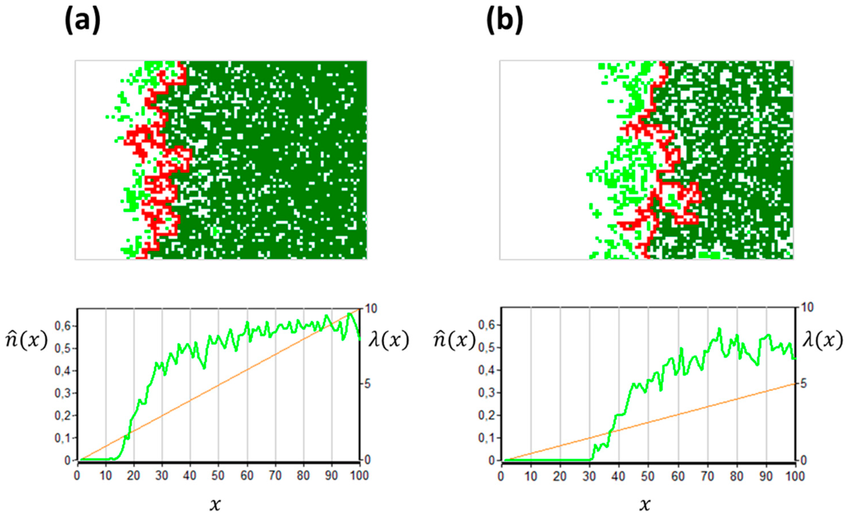
According to the results, the gRM and the gCP share some features. There is a characteristic mainland-with-islands structure along the gradient, where the mainland corresponds to the giant cluster, and the islands to the smaller clusters (Figure 1). Figure 1 shows snapshots from simulations in relatively small lattices (N = 6800). The results presented in References [31,59] were obtained in larger systems (N > 16 million). In the simulations, I used a four-cell neighborhood. Colonization was offspring-dependent; thus, was sufficient for characterizing the environment. The lower panels demonstrate the abrupt decline of (green curve) in spite of the smooth change of (orange line).
The upper panels show the spontaneous fragmentation at the range margin, depending on the slope (compare Figure 1a,b). These observations suggest that the occurrence of population fragments (islands) at a margin does not necessarily indicate any heterogeneity in the background (e.g., patches with particularly favorable microclimate or resource-richness [29,32]). Islands may emerge simply due to the internal dynamics. The two cases, externally vs. internally generated islands, can be distinguished by observing the positions of the islands over time. In the externally generated case, the islands are static (anchored to the favorable habitat patches), while, in the internally generated case, they are mobile.
In concert with the percolation model, many other models of gradient metapopulations produced mainland-and-archipelago structures, both within the gCP modeling framework [32,33], and outside [34,35,36,38,39,54,55]. I am not aware of any empirical study in which the external vs. internal reasons for island-formation were separated. I think this would be an important matter for future research, for example, for better understanding gene flow between the islands and the mainland, which hinges on the frequency of merging and splitting (see Section 1).
The sizes of the islands (population fragments) are also important. For example, genetic drift is more likely in smaller fragments, and local adaptation may be more difficult due to a lower local genetic diversity (c.f. [18]). On the other hand, these islands, as “outposts”, may become sources of population expansion in case of a climate change [51]. Percolation theory has some definite predictions about the sizes of the islands (Equations (6) and (7); see more details in Reference [31])). The sizes are predicted to decrease abruptly with the increase of distance from the mainland, depending on the slope. Observations at an alpine treeline in the Glacier National Park in North America [39] are in agreement with this prediction. The cumulative size distribution of the islands was found to fit a scaling law,
where the left side is the frequency of the patches that are larger than z. The value of the exponent was estimated to be ϕ = 0.83. The generality of this result in other range margins is yet to be explored. Considering the universality of the scaling laws that characterize the sizes of the islands in the gCP (Equations (6) and (7)), it would be interesting to study the cumulative size distribution of the islands in the gCP, and in other simulated and real range margins.
There are some mechanisms which decrease the likelihood of island-formation, for example, a strong Allee effect [9,35,36,38,40,60] or other local positive feedback mechanisms (self-facilitation [61]). In these cases, the gCP can be considered as a reference to which the other cases, with additional effects, can be compared.
It should be noted that the sizes of the gaps, which are left unoccupied by the species within the mainland, are also important in an ecological and evolutionary sense. The gaps were studied in non-gradient cases both in lattice simulations and on real-life data (in a multi-species situation, in a rainforest in Panama [62,63]). It would be interesting to extend these studies to range margins as well. Equations (2) and (3) predict an abrupt loss of gaps from the edge toward the inside of the mainland, and Equation (7) suggests that the number and area of islands within the mainland also decreases rapidly as the distance from the percolation threshold increases. Gaps in the canopy of the dominant species are important for the survival and reproduction of subordinate species, and they may provide special microclimatic conditions which increase biodiversity. Furthermore, they may be important in the evolutionary adaptation of the dominant species to the environment. Turner and Wong [54] applied stochastic simulations to investigate the problem that a mutation that would be advantageous within a certain range along an environmental gradient may arise further away from that range. The persistence of the mutant genotype hinges on its success of reaching the suitable sites, by percolating through the area covered by the resident genotype(s) (see also References [16,64,65]). This strongly depends on the density of the resident along the environmental gradient. The availability of empty gaps may be decisive in the percolation process.
5. The Hull Edge
The previous chapters presented the abrupt nature of the transition from the living to the extinct state along the gradient (as shown in the lower panels in Figure 1). The transition zone is relatively narrow, but has some interesting properties in magnification. Section 4 already presented some features of the islands. This chapter focuses on the edge of the mainland.
One of the frequently studied geometric structures is the hull. It consists of those sites which belong to the mainland, and are adjacent to sites that belong to the giant unoccupied site (the “ocean”); thus, the hull can be considered as the “coast” (marked by red in Figure 1). The neighborhood size (Z) at determining the clusters is arbitrary again, and is not necessarily the same as the neighborhood size used when producing the pattern in the gCP. The concept of the hull is broadly applied in percolation theory [66], beyond the gCP.
Figure 1 illustrates the winding of the hull in the gCP. The winding is constrained in the x direction by the gradient. The gradient imposes an inevitable finite-size effect, as it occurs even when the total area is infinite. At coarse spatial scales, the hull can be considered as a one-dimensional object (a straight line). At fine spatial scales, however, it has an intriguing fractal structure. The fractal dimension was numerically estimated to be D = 7/4 [31].
Coarsening the scale of observation, there is a crossover from D = 7/4 to 1 (Figure 4 in Reference [31]). Within the fractal region, D = 7/4 is independent of the neighborhood size Z, of the slope g (in ), and of some local details of the metapopulation dynamics; both a constant c with linear e(x), and a constant 1/e with linear c(x) yield the same fractal dimension. The independence is observable only within reasonable limits because of the aforementioned finite-size effect. Z or g is obviously too high when islands do not occur beyond the tips of the “peninsulas” of the hull, i.e., it can be suspected that the hull is distorted.
The (relative) independence of D on Z suggests that there is a zone (a range within x) in which the fractal properties are detectable. This may explain the scaling law observed by Zeng and Malanson [39] concerning the size distribution of the islands in a broad range of x (Equation (8)). This is an interesting matter for future research. The fractal nature of range margins is certainly an important finding, especially when the organism under study provides habitat for other organisms (for example, trees are inhabited by many organisms). Several papers in landscape ecology emphasized the importance of flows across boundaries (e.g., the diffusion of nutrients and of living organisms [28,67]). Milne et al. [34] discussed the importance of the hull in this regard. To my knowledge, we were the first to estimate the fractal dimension of the hull [31]. Such a high-dimensional fractal, D = 7/4, may provide a considerable surface for the flows.
Winding hull edges were observed, for example, at the margin of woodland patches in New Mexico [31,34]. The field data were fitted to the predicted D = 7/4 in Reference [31]. The fit was remarkably accurate at three different values of Z, which indicates the relevance of the theoretical results under natural conditions, even in relatively small systems.
The width (u) and length (w) of the hull are also important observables. The width was characterized by the standard deviation of the hull along the x axis. The length was defined as the number of lattice cells that belonged to the hull. Both the width and the length depend on g,
The scaling exponents are ζ = 3/7 and ω = 4/7. These values, as well as the fractal dimension D can be directly calculated from the scaling exponents β and γ in ordinary, non-gradient percolation (Equations (5) and (6); see pages 31 and 34 in Reference [31]). This is surprising, since the CP is a rather complex pattern-generating mechanism compared to the conventional generation of a percolation map (Section 4). The CP produces a clumped spatial distribution of occupied sites. The result can probably be explained by the abrupt decrease of spatial correlations away from the extinction threshold (Equation (3)). When g is not very large, i.e., the slope is not very steep, then the hull is at a considerable distance from the extinction threshold (see Figure 1b) and, thus, the spatial correlations may become negligible. Essentially, the system becomes similar to a gradient random map. This hypothesis was confirmed by analyzing the hull in the gRM. Exactly the same values of the scaling exponents (D = 7/4, ζ = 3/7, and ω = 4/7) were found. This suggests that the gRM, in spite of its simplicity, may be a suitable model for the study of the hull across a gradient, even in those cases in which the underlying population dynamic process is more complex. It would be an interesting task for future research to check the validity of this statement in gradient metapopulation models that are more complex than the gCP. The fractal dimension of the hull could certainly be estimated in real range margins as well. Obtaining data for u(g) and w(g) is more difficult.
Finally, the mean position of the hull along the x axis is also an important observable (let us denote it by xm). This can be considered as the main place of the transition from the connected to the fragmented state. Accordingly, Milne et al. [34] raised the hypothesis that the density of occupied sites at this place is . In square lattices, considering only the most adjacent cells as neighbors (Z = 4), this value is approximately pc ≈ 0.59 (see Section 4 and Reference [57]). The hypothesis was confirmed by gRM simulations, and similar values were also found in the studied New Mexican woodlands [31,34]. It is remarkable that, in forestry, 60% canopy cover is often used as a limit above which the vegetation can be considered a closed forest [34].
Although gradient metapopulations are fairly complex (see the previous sections), the hull appears to be a simple structure. It is hopeful to understand its main features solely on the basis of classical percolation theory. We investigated the validity of this statement by simulating percolation maps with various p(x) functions, in addition to the previously studied linear . The simulations confirmed the broad validity of D = 7/4. The investigations also provided an asymptotic expression for the probability that a site at a given distance from xm is on the hull [59]. Within the complex pattern of the range margin (Figure 1), xm is a well-defined position. It could be used for delineating the range edge unequivocally, and monitoring the shift of the range in case of a climate change [31,34]. I think it is an important matter for future research to explore this opportunity in various species, and to work out a monitoring method that could be used in practice.
6. Summary and Outlook
Understanding the limits of species’ distributions is one of the fundamental goals in ecology. The task is rather difficult, because the range edges are often self-organized, i.e., broader geographic patterns emerge from the local processes in a complex manner [4,9,29,31,32,33,34,38,39,47,52,53,56,68,69]. Comparisons between different species and geographic regions necessitate a common theoretical framework, within which this complexity could be handled. Several papers suggest that the theory of phase transitions provides important help in this attempt [31,34,39,52,53,70,71]. It suggests some broadly generalizable laws, which concern the spatial pattern of occupied sites along environmental gradients.
The theory also suggests some direct simplifications, which reduce complexity. One of these is the use of the hull for delineating the range edge. The hull has some broadly applicable scaling properties, which were proven to be independent of the details of the models, as they could be deduced from ordinary (non-gradient) percolation. These theoretical considerations suggest that the comparison of range margins (between species, places, or years) could be simplified by comparing the hulls. For example, a range shift could be detected sensitively by monitoring the mean position of the hull.
Another opportunity for simplification is suggested by the gCP, and concerns the equilibrium density profile along the gradient, . Computer simulations raised the hypothesis that the spreading rate, , is sufficient for predicting the densities in a broad range of realistic cases; thus, various combinations of c(x) and e(x) with the same produce the same equilibrium density profile. The possibility of this kind of simplification, by rescaling time, could be investigated in other gradient metapopulation models as well, beyond the gCP.
I presented two phase transitions: (1) from the living to the extinct state, and (2) from the connected to the fragmented one. Each transition was presented firstly in homogeneous (non-gradient) systems. Then, an environmental gradient was introduced, i.e., it was assumed that the control parameter changed along a spatial axis. The gradient resulted in some inevitable finite-size effects which blurred the original threshold-like transition. Nevertheless, the changes remained abrupt even along smooth gradients. This “sharpening” is an important phenomenon, as it can influence the population’s adaptability to the environment, and the capacity of movement in case of climate change.
This review was based on the gradient contact process (gCP), which is a basic model of colonization and extinction across an environmental gradient. Its main findings are in agreement with many other, more complex gradient metapopulation models. It would be interesting to outline the set of models to which the gCP’s universal features are directly applicable, and to understand those factors that call for fundamental changes in the model’s settings, thus making the gCP’s scaling laws inapplicable. For example, some papers suggest that a strong Allee effect can destroy the CP’s phase transition [40] and can fundamentally change the metapopulations spatial structure [38,40,60]. Positive feedback mechanisms between the organism and the environment (e.g., Reference [61]) require special attention, because they can generate spatial patterns that are fundamentally different from those that are generated by the gCP [72]. The gCP’s transition from the living to the extinct state hinges on the emergent spatial pattern. Background heterogeneity in addition to the gradient (e.g., the occurrence of non-habitable or less habitable patches) can also disturb the phase transition [73], depending on the quality, amount, size, shape, and persistence of the patches (see some examples in References [28,74]). These effects also require further investigation.
Understanding the fine-scale structure and dynamics of range margins is indispensable for predicting the ecological effects of climate changes. Due to the rapidity of anthropogenic changes, we need predictions even on the fine scale of years or decades. Considering the usually limited capacity for data collection in the field, good models are pivotal for predictions and monitoring. I think that linking ecological knowledge with the theory of phase transitions can advance this research significantly.
Funding
This research was funded by NKFIH-OTKA, grant numbers K109215 and K124438.
Acknowledgments
I am grateful to Michael Gastner and Máté Gulyás for valuable comments on the manuscript.
Conflicts of Interest
The author declares no conflicts of interest.
References
- Elton, C.S. Animal Ecology and Evolution; Clarendon Press: Oxford, UK, 1930. [Google Scholar]
- Andrewartha, H.G.; Birch, L.C. The Distribution and Abundance of Animals; University of Chicago Press: Chicago, IL, USA, 1954. [Google Scholar]
- Travis, J.M.J. Climate change and habitat destruction: A deadly anthropogenic cocktail. Proc. R. Soc. Lond. B 2003, 270, 467–473. [Google Scholar] [CrossRef] [PubMed]
- Holt, R.D.; Keitt, T.H. Species’ borders: A unifying theme in ecology. Oikos 2005, 108, 3–6. [Google Scholar] [CrossRef]
- Geber, M.A. To the edge: Studies of species’ range limits. New Phytol. 2008, 178, 228–230. [Google Scholar] [CrossRef] [PubMed]
- Mustin, K.; Benton, T.G.; Dytham, C.; Travis, J.M.J. The dynamics of climate-induced range shifting; perspectives from simulation modelling. Oikos 2009, 118, 131–137. [Google Scholar] [CrossRef]
- Geber, M. Ecological and evolutionary limits to species geographic ranges. Am. Nat. 2011, 178, S1–S5. [Google Scholar] [CrossRef] [PubMed]
- Eppinga, M.B.; Pucko, C.A.; Baudena, M.; Beckage, B.; Molofsky, J. A new method to infer vegetation boundary movement from ‘snapshot’ data. Ecography 2013, 36, 622–635. [Google Scholar] [CrossRef]
- Kubisch, A.; Holt, R.D.; Poethke, H.J.; Fronhofer, E.A. Where am I and why? Synthesizing range biology and the eco-evolutionary dynamics of dispersal. Oikos 2014, 123, 5–22. [Google Scholar] [CrossRef]
- Tejo, M.; Niklitschek-Soto, S.; Vásquez, C.; Marquet, P.A. Single species dynamics under climate change. Theor. Ecol. 2017, 10, 181–193. [Google Scholar] [CrossRef]
- Bocedi, G.; Palmer, S.C.; Pe’er, G.; Heikkinen, R.K.; Matsinos, Y.G.; Watts, K.; Travis, J.M.; Freckleton, R. RangeShifter: A platform for modelling spatial eco-evolutionary dynamics and species’ responses to environmental changes. Methods Ecol. Evol. 2014, 5, 388–396. [Google Scholar] [CrossRef]
- Crawford, R.M.M. Plants at the Margin. Ecological Limits and Climate Change; Cambridge University Press: Cambridge, UK, 2008. [Google Scholar]
- Nagy, L.; Grabherr, G. The Biology of Alpine Habitats; Oxford University Press: Oxford, UK, 2009. [Google Scholar]
- Chuang, A.; Peterson, C.R. Expanding population edges: Theories, traits, and trade-offs. Glob. Chang. Biol. 2016, 22, 494–512. [Google Scholar] [CrossRef]
- Vucetich, J.A.; Waite, T.A. Spatial patterns of demography and genetic processes across the species’ range: Null hypotheses for landscape conservation genetics. Conserv. Genet. 2003, 4, 639–645. [Google Scholar] [CrossRef]
- Atkins, K.E.; Travis, J.M.J. Local adaptation and the evolution of species ranges under climate change. J. Theor. Biol. 2010, 266, 449–457. [Google Scholar] [CrossRef]
- Kubisch, A.; Fronhofer, E.A. Dispersal, evolution and range dynamics—A synthesis. Oikos 2014, 123, 3–4. [Google Scholar] [CrossRef]
- Polechová, J.; Barton, N. Limits to adaptation along environmental gradients. Proc. Natl. Acad. Sci. USA 2015, 112, 6401–6406. [Google Scholar] [CrossRef] [PubMed]
- Kirkpatrick, M.; Barton, N. Evolution of a species’ range. Am. Nat. 1997, 150, 1–23. [Google Scholar] [CrossRef] [PubMed]
- Sexton, J.P.; McIntyre, P.J.; Angert, A.L.; Rice, K.J. Evolution and ecology of species range limits. Ann. Rev. Ecol. Syst. 2009, 40, 415–436. [Google Scholar] [CrossRef]
- Holling, C.S. The strategy of building models of complex ecological systems. In Systems Analysis in Ecology; Watt, K.E.F., Ed.; Academic Press: New York, NY, USA, 1966; pp. 195–214. [Google Scholar]
- Whittaker, R.H. Gradient analysis of vegetation. Biol. Rev. 1967, 42, 207–264. [Google Scholar] [CrossRef] [PubMed]
- Hanski, I. Metapopulation Ecology; Oxford University Press: Oxford, UK, 1999. [Google Scholar]
- Levins, R. Some demographic and genetic consequences of environmental heterogeneity for biological control. Bull. Entomol. Soc. Am. 1969, 15, 237–240. [Google Scholar] [CrossRef]
- Tilman, D.; Kareiva, P. (Eds.) Spatial Ecology: The Role of Space in Population Dynamics and Interspecific Interactions; Princeton University Press: Princeton, NJ, USA, 1997. [Google Scholar]
- Czárán, T. Spatiotemporal Models of Population and Community Dynamics; Chapman and Hall: London, UK, 1998. [Google Scholar]
- Harris, T.E. Contact interactions on a lattice. Ann. Prob. 1974, 2, 969–988. [Google Scholar] [CrossRef]
- Oborny, B.; Szabó, G.; Meszéna, G. Survival of species in patchy landscapes: Percolation in space and time. In Scaling Biodiversity; Storch, D., Marquet, P., Brown, J., Eds.; Cambridge University Press: Cambridge, UK, 2007; pp. 409–440. [Google Scholar]
- Oborny, B.; Vukov, J.; Csányi, G.; Meszéna, G. Metapopulation dynamics across gradients—The relation between colonization and extinction in shaping the range edge. Oikos 2009, 118, 1453–1460. [Google Scholar] [CrossRef]
- Noble, I.R. A model of the responses of ecotones to climate change. Ecol. Appl. 1993, 3, 396–403. [Google Scholar] [CrossRef] [PubMed]
- Gastner, M.; Oborny, B.; Pruessner, G.; Zimmermann, D. Transition from connected to fragmented vegetation across an environmental gradient: Scaling laws in ecotone geometry. Am. Nat. 2009, 174, 23–39. [Google Scholar] [CrossRef] [PubMed]
- Lennon, J.; Turner, J.R.G.; Connell, D. A metapopulation model of species boundaries. Oikos 1997, 78, 486–502. [Google Scholar] [CrossRef]
- Holt, R.D.; Keitt, T.H. Alternative causes for range limits: A metapopulation perspective. Ecol. Lett. 2000, 3, 41–47. [Google Scholar] [CrossRef]
- Milne, B.T.; Johnson, A.R.; Keitt, T.H.; Hatfield, C.A.; David, J.; Hraber, P.T. Detection of critical densities associated with pinon-juniper woodland ecotones. Ecology 1996, 77, 805–821. [Google Scholar] [CrossRef]
- Wilson, W.G.; Nisbet, R.M.; Ross, A.H.; Robles, C.; Desharnais, R.A. Abrupt population change along smooth environmental gradients. Bull. Math. Biol. 1996, 58, 907–922. [Google Scholar] [CrossRef]
- Antonovics, J.; McKane, A.J.; Newman, T.J. Spatiotemporal dynamics in marginal populations. Am Nat. 2006, 167, 16–27. [Google Scholar] [CrossRef] [PubMed]
- Case, T.J.; Holt, R.D.; McPeek, M.A.; Keitt, T.H. The community context of species’ borders: Ecological and evolutionary perspectives. Oikos 2005, 108, 28–46. [Google Scholar] [CrossRef]
- Holt, R.D.; Keitt, T.H.; Lewis, M.A.; Maurer, B.A.; Taper, M.L. Theoretical models of species’ borders: Single species approaches. Oikos 2005, 108, 18–27. [Google Scholar] [CrossRef]
- Zeng, Y.; Malanson, G.P. Endogenous fractal dynamics at alpine treeline ecotones. Geogr. Anal. 2006, 38, 271–287. [Google Scholar] [CrossRef]
- Gastner, M.; Oborny, B.; Ryabov, A.B.; Blasius, B. Changes in the gradient percolation transition caused by an Allee effect. Phys. Rev. Lett. 2011, 106, 128103. [Google Scholar] [CrossRef] [PubMed]
- Ovaskainen, O.; Hanski, I. Spatially structured metapopulation models: Global and local assessment of metapopulation capacity. Theor. Popul. Biol. 2001, 60, 281–302. [Google Scholar] [CrossRef] [PubMed]
- Broadbent, S.R.; Hammersley, J.M. Percolation processes. I. Chrystals and mazes. Proc. Camb. Phil. Soc. 1957, 53, 629–645. [Google Scholar] [CrossRef]
- Marro, J.; Dickman, R. Nonequilibrium Phase Transitions in Lattice Models; Cambridge University Press: Cambridge, UK, 1999. [Google Scholar]
- Hinrichsen, H. Non-equilibrium critical phenomena and phase transitions into absorbing states. Adv. Phys. 2000, 49, 815–958. [Google Scholar] [CrossRef] [Green Version]
- Stanley, H.E. Introduction to Phase Transitions and Critical Phenomena; Clarendon Press: Oxford, UK, 1971. [Google Scholar]
- Oborny, B.; Meszéna, G.; Szabó, G. Dynamics of populations on the verge of extinction. Oikos 2005, 109, 291–296. [Google Scholar] [Green Version]
- Lawton, J.H. Range, population abundance and conservation. TREE 1993, 8, 409–413. [Google Scholar] [CrossRef]
- Brooks, T. Living on the edge. Nature 2000, 403, 26–28. [Google Scholar] [CrossRef]
- Caughley, G.D.; Grice, D.; Barker, R.; Brown, B. The edge of the range. J. Anim. Ecol. 1988, 57, 771–785. [Google Scholar] [CrossRef]
- Allen, C.D.; Breshears, D.D. Drought-induced shift of a forest–woodland ecotone: Rapid landscape response to climate variation. Proc. Natl. Acad. Sci. USA 1998, 95, 14839–14842. [Google Scholar] [CrossRef]
- Camarero, J.J.; Linares, J.C.; García-Cervigón, A.I.; Batllori, E.; Martínez, I.; Gutiérrez, E. Back to the future: The responses of alpine treelines to climate warming are constrained by the current ecotone structure. Ecosystems 2017, 20, 683–700. [Google Scholar] [CrossRef]
- Loehle, C.; Li, B.-L.; Sundell, R.C. Forest spread and phase transitions at forest-prairie ecotones in Kansas, USA. Landsc. Ecol. 1996, 11, 225–235. [Google Scholar] [CrossRef]
- Li, B.-L. A theoretical framework of ecological phase transitions for characterizing tree-grassland dynamics. Acta Biotheor. 2002, 50, 141–154. [Google Scholar] [CrossRef] [PubMed]
- Turner, J.R.G.; Wong, H.Y. Why do species have a skin? Investigating mutational constraint with a fundamental population model. Biol. J. Linn. Soc. 2010, 101, 213–227. [Google Scholar] [CrossRef] [Green Version]
- Buckley, H.L.; Case, B.S.; Vallejos, R.; Camarero, J.J.; Gutiérrez, E.; Liang, E.; Wang, Y.; Ellison, A.M. Detecting ecological patterns along environmental gradients: Alpine treeline ecotones. Chance 2016, 29, 10–15. [Google Scholar] [CrossRef]
- Brown, J.H.; Stevens, G.C.; Kaufman, D.M. The geographic range: Size, shape, boundaries and internal structure. Ann. Rev. Ecol. Syst. 1996, 27, 597–623. [Google Scholar] [CrossRef]
- Stauffer, D.; Aharony, A. Introduction to Percolation Theory; Taylor & Francis: Boca Raton, FL, USA, 1992. [Google Scholar]
- Zallen, R. Introduction to percolation: A model for all seasons. In Percolation Structures and Processes; Deutscher, G., Zallen, R., Adler, J., Eds.; Israel Physical Society: Jerusalem, Israel, 1983. [Google Scholar]
- Gastner, M.; Oborny, B. The geometry of percolation fronts in two-dimensional lattices with spatially varying densities. New J. Phys. 2012, 14, 103019. [Google Scholar] [CrossRef] [Green Version]
- Keitt, T.H.; Lewis, M.A.; Holt, R.D. Allee effects, invasion pinning, and species’ borders. Am. Nat. 2001, 157, 203–216. [Google Scholar]
- Malanson, G.P.; Zeng, Y. Uncovering spatial feedbacks at alpine treeline using spatial metrics in Evolutionary Simulations. In GeoDynamics; CRC Press: Boca Raton, FL, USA, 2004; pp. 137–150. [Google Scholar]
- Manrubia, S.C.; Solé, R.V. On forest spatial dynamics with gap formation. J. Theor. Biol. 1997, 187, 159–164. [Google Scholar] [CrossRef]
- Solé, R.V.; Bartumeus, F.; Gamarra, J.G.P. Gap percolation in rainforests. Oikos 2005, 110, 177–185. [Google Scholar] [CrossRef] [Green Version]
- McInerny, G.J.; Turner, J.R.; Wong, H.Y.; Travis, J.M.; Benton, T.G. How range shifts induced by climate change affect neutral evolution. Proc. R. Soc. B 2009, 276, 1527–1534. [Google Scholar] [CrossRef] [Green Version]
- Peischl, S.; Kirkpatrick, M.; Excoffier, L. Expansion load and the evolutionary dynamics of a species range. Am. Nat. 2015, 185, E81–E93. [Google Scholar] [CrossRef] [PubMed]
- Grossman, T.; Aharony, A. Structure and perimeters of percolation clusters. J. Phys. A Math. Gen. 1986, 19, L745. [Google Scholar] [CrossRef]
- Wiens, J.A. Ecological flows across landscape boundaries: A conceptual overview. In Landscape Boundaries. Ecological Studies (Analysis and Synthesis) Vol. 92; Hansen, A.J., di Castri, F.M., Eds.; Springer: New York, NY, USA, 1992. [Google Scholar]
- Milne, B. Motivation and benefits of complex systems approaches in ecology. Ecosystems 1998, 1, 449. [Google Scholar] [CrossRef]
- Maurer, B.A.; Taper, M.L. Connecting geographical distributions with population processes. Ecol. Lett. 2002, 5, 223–231. [Google Scholar] [CrossRef]
- Johnson, A.R.; Milne, B.T.; Hraber, P. Analysis of change in pinon-juniper woodlands based on aerial photography, 1930’s-1980’s. In Rio Grande Ecosystems: Linking Land, Water, and People; Finch, D.M., Whitney, J.C., Kelly, J.F., Loftin, S.R., Eds.; U.S. Department of Agriculture, Forest Service: Washington, DC, USA, 1999; pp. 106–111. [Google Scholar]
- Solé, R.V. Phase Transitions; Princeton University Press: Princeton, NJ, USA, 2011. [Google Scholar]
- Bekker, M.F.; Malanson, G.P. Linear forest patterns in subalpine environments. Prog. Phys. Geogr. 2008, 32, 635–653. [Google Scholar] [CrossRef]
- Szabó, G.; Gergely, H.; Oborny, B. Generalized contact process on random environments. Phys. Rev. E 2002, 65, 066111. [Google Scholar] [CrossRef] [PubMed]
- Keymer, J.E.; Marquet, P.A.; Velasco-Hernández, J.X.; Levin, S.A. Extinction thresholds and metapopulation persistence in dynamic landscapes. Am. Nat. 2000, 156, 478–494. [Google Scholar] [CrossRef]
Figure 1.
Snapshots from gradient contact processes with two different slopes. The lattice size is N = 6800 cells (100 × 68). The boundaries between the lattice cells are not shown. The environment changes linearly along the horizontal axis, , ranging from 0 to (a) 10 or (b) 5. In each case, the upper panel shows the spatial pattern of the occupied sites. The islands are light green. The mainland is subdivided into those cells which belong to the hull (red) and the other cells (dark green). Note that islands occur even within the area dominated by the mainland. The lower panel presents , the density of occupied sites in each column in the lattice (light green curve; left axis), and (orange line; right axis).

© 2018 by the author. Licensee MDPI, Basel, Switzerland. This article is an open access article distributed under the terms and conditions of the Creative Commons Attribution (CC BY) license (http://creativecommons.org/licenses/by/4.0/).
Share and Cite
MDPI and ACS Style
Oborny, B. Scaling Laws in the Fine-Scale Structure of Range Margins. Mathematics 2018, 6, 315. https://doi.org/10.3390/math6120315
AMA Style
Oborny B. Scaling Laws in the Fine-Scale Structure of Range Margins. Mathematics. 2018; 6(12):315. https://doi.org/10.3390/math6120315
Chicago/Turabian StyleOborny, Beáta. 2018. "Scaling Laws in the Fine-Scale Structure of Range Margins" Mathematics 6, no. 12: 315. https://doi.org/10.3390/math6120315
Note that from the first issue of 2016, this journal uses article numbers instead of page numbers. See further details here.