Analysis of PFG Anomalous Diffusion via Real-Space and Phase-Space Approaches

Abstract

Pulsed-field gradient (PFG) diffusion experiments can be used to measure anomalous diffusion in many polymer or biological systems. However, it is still complicated to analyze PFG anomalous diffusion, particularly the finite gradient pulse width (FGPW) effect. In practical applications, the FGPW effect may not be neglected, such as in clinical diffusion magnetic resonance imaging (MRI). Here, two significantly different methods are proposed to analyze PFG anomalous diffusion: the effective phase-shift diffusion equation (EPSDE) method and a method based on observing the signal intensity at the origin. The EPSDE method describes the phase evolution in virtual phase space, while the method to observe the signal intensity at the origin describes the magnetization evolution in real space. However, these two approaches give the same general PFG signal attenuation including the FGPW effect, which can be numerically evaluated by a direct integration method. The direct integration method is fast and without overflow. It is a convenient numerical evaluation method for Mittag-Leffler function-type PFG signal attenuation. The methods here provide a clear view of spin evolution under a field gradient, and their results will help the analysis of PFG anomalous diffusion.

1. Introduction

Anomalous dynamic behavior exists in many polymer or biological systems [1,2,3,4,5,6]. These systems often consist of various molecules such as macromolecules and small penetrant molecules like water. These molecules often demonstrate anomalous dynamics behavior: their rotational motion time constants usually obey a stretched exponential distribution, namely, the Kohlrausch–Williams–Watts (KWW) function distribution [7,8], and their translational diffusion jump time and jump length could follow power law distributions [2]. Nuclear magnetic resonance (NMR) is one of the important techniques used to detect these anomalous dynamic behaviors. For instance, anomalous diffusion can be detected by pulsed-field gradient (PFG) NMR experiments.

PFG diffusion NMR [9,10,11,12,13,14,15] has been a powerful tool for measuring normal diffusion. The history of using a field gradient to measure diffusion can be tracked back to Hahn, who first observed the influence of the molecule diffusion under a gradient magnetic field upon echo amplitudes in 1950 [9]. PFG diffusion measurements have broad applications in NMR and magnetic resonance imaging (MRI) [13,14,15,16]. For instance, the water diffusion difference in different parts of the brain can be used as an important contrast factor to build imaging of acute strokes [16]. The PFG technique, being an ultra-valuable tool for normal disunion, could play an increasingly important role in monitoring anomalous diffusion occurring in many polymer and biological systems.

PFG anomalous diffusion [17,18,19,20,21,22,23] is different from PFG normal diffusion. Unlike normal diffusion, anomalous diffusion has a non-Gaussian probability distribution [2,24], and its mean square displacement is not linearly proportional to diffusion time [2]. These non-Gaussian characteristics make it complicated to analyze PFG anomalous diffusion. Although PFG anomalous diffusion can be approximately analyzed by traditional methods such as the apparent diffusion coefficient method, PFG theories based on the fractional derivative could not only improve the analysis accuracy on the diffusion domain size, diffusion constant, and other variables [17,18,25,26,27,28], but also yield additional information such as the time derivative order α and space derivative order β that are related with diffusion jump time and jump length distributions determined by material properties.

Much effort has been devoted to studying PFG anomalous diffusion based on fractional calculus, which includes the propagator method [29], the modified Bloch equation method [17,25,30,31], the effective phase-shift diffusion equation (EPSDE)method [18], the instantaneous signal attenuation method [26], the modified-Gaussian or non-Gaussian distribution method [27], etc. Additionally, PFG anomalous diffusions in restricted geometries such as plate, sphere, and cylinder have been investigated [28]. These theoretical methods analyze PFG anomalous diffusion from different angles. Therefore, each of them can have its own advantages in handling certain types of PFG anomalous diffusion. To better apply the PFG technique to studying anomalous diffusion, it is still valuable to develop new theoretical treatments for PFG anomalous diffusion.

In this paper, two methods based on the fractional derivative [1,2,6,32,33,34] are proposed to give general analytical PFG signal attenuation expressions for anomalous diffusion. The first method is the recently developed EPSDE method [18]. This method describes the spin phase evolution by an effective phase diffusion process in virtual phase space [18]. Solving the EPSDE gives valuable information about the phase evolution process such as the phase probability distribution function and the moment of mean phase displacement. Meanwhile, other conventional methods render it difficult to get this phase information, and usually assume an approximate phase distribution such as Gaussian phase distribution [13]. In this paper, it will be shown that a solvable PFG signal attenuation equation can be derived by applying a Fourier transform to the effective phase-shift equation. The second method is to observe the signal intensity at the origin, and is an ultra-simple new method. For a homogeneous diffusion spin system, although the magnetization amplitude attenuates because of the gradient magnetic field effect, the phase of magnetization keeps constant at the origin of the gradient field. Such a specific phase property is employed to derive a PFG signal attenuation equation in this paper. The above two methods give the same signal attenuation equation, from which the general PFG signal attenuation expression can be derived by the Adomian decomposition method [35,36,37,38,39]. Besides the Adomian decomposition method, a direct integration method was proposed for the numerical evaluation of the PFG signal attenuation, which is a fast and simple method. The results include the finite gradient pulse width (FGPW) effect [13,14,15], namely, the signal attenuation during each gradient pulse application period. Theoretically, during a short gradient pulse, the PFG signal attenuation can be neglected; nevertheless, the gradient pulse used in a clinical MRI is usually long [16,40]. Additionally, a longer gradient pulse allows the measuring of slower diffusion under the same gradient maximum intensity, which matters in the study of polymer and biological systems where the molecule diffusion is often slow. Therefore, we need to consider the FGPW effect in many real applications. The two methods here give the same results in terms of the FGPW effect. These results agree with reported results from some other methods [18,26,27] and the continuous time random walk simulation [26,29]. Furthermore, PFG anomalous diffusion of intramolecular multiple quantum coherence (MQC) is also discussed [27]. The MQC effect has the benefit of enhancing the gradient effect on PFG signal attenuation [41]. The two methods provide complementary views of PFG anomalous diffusion from both the real space and phase space.

2. Theory

2.1. The Phase-Space Method: The Effective Phase-Shift Diffusion Method

For the sake of simplicity, only one-dimensional anomalous diffusion is considered in this paper. In PFG experiments, the field gradient pulse results in a time- and space-dependent magnetic field $B(z,t)=B_0+g(t)\cdot z$, where $B_0$ is the exterior magnetic field, z is the position, and $g(t)$ is the time-dependent gradient [13,14,15]. The magnetic field exerts a torque on each spin moment. The torque changes the spin angular momentum direction, which leads the spin to precess about the magnetic field with Larmor frequency $\omega (z,t)=-\gamma B(z,t).$ In a rotating frame with angular frequency ${\omega }_0=-\gamma B_0$, a diffusing spin at position $z(t^{\prime })$ has a time-dependent angular frequency $\gamma g(t^{\prime })\cdot z(t^{\prime })$, and its phase accumulated along the diffusion path is [13,14,15,19]

$$\varphi (t)=-{\displaystyle {\int }_0^t\gamma g(t^{\prime })\cdot z}(t^{\prime })d{t}^{\prime },$$

(1)

where $\varphi (t)$ is the net-accumulating phase. The range of $\varphi (t)$ is $-\infty <\varphi (t)<\infty$ rather than $-\pi \le \varphi (t)\le \pi$, and $\cos (\varphi (t))$ is the projection factor of the spin magnetization to the observing coordinate axis. The PFG signal comes from the ensemble contribution from all spins by averaging over all possible phases [13,14,15]:

$$S(t)=S(0){\displaystyle {\int }_{-\infty }^{\infty }P(\varphi ,t)\exp (+i\varphi )d\varphi },$$

(2)

where $S(0)$ is the signal intensity at the beginning of the first gradient pulse, $S(t)$ is the signal intensity at time t, and $P(\varphi ,t)$ is the accumulating phase probability distribution function. In a symmetric diffusion system, Equation (2) can be further written as

$$S(t)=S(0){\displaystyle {\int }_{-\infty }^{\infty }P(\varphi ,t)\cos (\varphi )d\varphi }.$$

(3)

Because the NMR signal comes from numerous spins, the percentage of spins with potentially infinite $\varphi (t)$ is very small, and can therefore be neglected. Additionally, $-1\le \cos (\varphi (t))\le 1$; therefore, $0\le \left|S(t)\right|\le S(0)$, and $S(t)$ is a finite quantity that can be measured in NMR experiments. A possibly infinite “mean square phase displacement” $\langle {\left|\varphi (t)\right|}^{\beta }\rangle$ is not necessarily an obstacle in PFG NMR measurement, although it may have a significant effect in other academic fields. The PFG signal attenuation can be obtained based on Equation (2) or (3), but the phase evolution process based on the phase path integral Equation (1) is complicated. Nevertheless, the recently developed EPSDE method provides a simple way to describe the phase evolution based on an effective phase diffusion process [18]. In the following, the effective phase diffusion equation method [18] will be briefly reintroduced. Additionally, a general solution including the FGPW effect will be given that has not been reported in [18].

For simplicity, only diffusion with a symmetric probability distribution is studied here. The self-diffusion process can be described by a random walk, which consists of a sequence of independent random jumps with waiting times $\Delta t_1$, $\Delta t_2$, $\Delta t_3$,…, $\Delta t_n$, and corresponding displacement lengths $\Delta z_1$, $\Delta z_2$, $\Delta z_3$,…, $\Delta z_n$. Based on the random walk, Equation (1) can be rewritten as [18]

$$\begin{array}{ll}\varphi (t_{tot})& =-{\displaystyle \sum _{i=1}^n\gamma \Delta t_{i}g(t_i)\cdot \left({\displaystyle \sum _{m=1}^i\Delta z_m}+z_0\right)}\\ & =-\gamma {\displaystyle \sum _{m=1}^n\left[{\displaystyle \sum _i^n\Delta t_{i}g(t_i)}-{\displaystyle \sum _i^{m-1}\Delta t_{i}g(t_i)}\right]\cdot \Delta z_m-\gamma {\displaystyle \sum _{i=1}^n\Delta t_{i}g(t_i)\cdot z_0}}\\ & =-{\displaystyle \sum _{m=1}^n\left[K(t)-K(t_{m-1})\right]\cdot \Delta z_m-K(t)\cdot z_0}\\ & =-{\displaystyle \sum _{m=1}^n\left[K(t)-K(t_m)\right]\cdot \Delta z_m-K(t)\cdot z_0}\end{array}$$

(4)

where

$$K(t)={\displaystyle {\int }_0^t\gamma g(t^{\prime })d{t}^{\prime }}$$

(5)

is the wavenumber [13,14,15]. In Equation (4), $K(t_m)\approx K(t_{m-1})$ is used because $\left[K(t_m)-K(t_{m-1})\right]\cdot \Delta z_m$ is negligible, and the temporal and spatial summation orders are interchanged because $\Delta t_{i}g(t_i)$ and $\Delta z_m$ are often noncorrelated. In most PFG experiments, $K(t_{tot})=0$ where $t_{tot}$ is the time at the end of the rephasing gradient pulse, so Equation (4) can be further simplified to [18]

$$\varphi (t_{tot})=-{\displaystyle \sum _{m}K(t_m)\cdot \Delta z_m}.$$

(6)

The $-{\displaystyle \sum _{m}K(t_m)\cdot \Delta z_m}$ term in Equation (6) is an effective phase random walk with a jump length $-K(t_m)\cdot \Delta z_m$ and a jump waiting time $\Delta t_m$ The phase random walk can be treated as an effective phase diffusion, and can be obtained from the corresponding spin diffusion in the real space by scaling the jump length $\Delta z(t)$ by a factor $-K(t)$. Because $\langle {\left|\Delta z\right|}^{\beta }\rangle /\langle \Delta t^{\alpha }\rangle \propto D_f$ and $\langle {\left|K(t)\Delta z\right|}^{\beta }\rangle /\langle \Delta t^{\alpha }\rangle \propto D_{\varphi eff}(t)$, the effective phase diffusion constant is $D_{\varphi eff}(t)=K^{\beta }(t)D_f$ (oftentimes $K(t)\ge 0$) [18], where $D_f$ and $D_{\varphi eff}(t)$ are the fractional diffusion coefficients for the real-space diffusion and the effective phase diffusion, respectively, and their units are $m^{\beta }/s^{\alpha }$ and $ra{d}^{\beta }/s^{\alpha }$. As both the effective phase diffusion and the real spin particle diffusion belong to the same type of diffusion, they should obey the same type of diffusion equation. The one-dimensional real-space diffusion equation based on the fractional derivative is [6,31,32,33,34]

$${}_t{D}_{*}^{\alpha }{M}_{xy}\left(z,t\right)=D_f\frac{{\partial }^{\beta }}{\partial {\left|z\right|}^{\beta }}{M}_{xy}\left(z,t\right),$$

(7)

where $M_{xy}\left(z,t\right)$ is the spin magnetization in PFG experiments, and ${}_t{D}_{*}^{\alpha }$ is the Caputo fractional derivative defined as [6,31,32,33,34]

$${}_t{D}_{*}^{\alpha }f(t):=\{\begin{array}{c}\frac{1}{\Gamma (m-\alpha )}{\displaystyle {\int }_0^t\frac{f^m(\tau )d\tau }{{(t-\tau )}^{\alpha +1-m}},m-1<\alpha <m}\\ \frac{d^m}{d{t}^m}f(t),\alpha =m\end{array}$$

(8)

and $\frac{{\partial }^{\beta }}{\partial {\left|z\right|}^{\beta }}$ is the space fractional derivative [6,31,32,33,34] defined in Appendix A. By replacing coordinate z with $\varphi$, and $D_f$ with $D_{\varphi eff}(t)$, respectively, from real-space diffusion Equation (9), the effective phase diffusion equations can be obtained [18] as

$${}_t{D}_{*}^{\alpha }P\left(\varphi ,t\right)=K^{\beta }(t)D_f\frac{{\partial }^{\beta }}{\partial {\left|\varphi \right|}^{\beta }}P\left(\varphi ,t\right).$$

(9)

As $\hat{F}\left\{f(x,t)\right\}=f(q,t)$ and $\hat{F}\left\{\frac{{\partial }^{\beta }}{\partial {\left|x\right|}^{\beta }}f(x,t);q\right\}=-q^{\beta }f(q)$ [31,32,33,34] where q is the wavenumber, applying a Fourier transform $\hat{F}\left\{f(x)\right\}={\displaystyle {\int }_{-\infty }^{\infty }f(x)\exp (+iqx)dx}$ to both sides of Equation (9) gives

$${}_t{D}_{*}^{\alpha }P\left(q,t\right)=-K^{\beta }(t)q^{\beta }{D}_{f}P\left(q,t\right),$$

(10)

which is a q-space phase diffusion equation. Here, q is the wavenumber dedicated to the above Fourier transform, which differs from the field gradient pulse-induced wavenumber $K(t)$ defined by Equation (5). When q = 1, $P\left(q,t\right)$ in Equation (10) equals the attenuated signal amplitude because, in PFG experiments, the signal attenuation can be calculated based on Equation (2) as [18]

$$S(t)=S(0){\displaystyle {\int }_{-\infty }^{\infty }P(\varphi ,t)\exp (+i\varphi )d\varphi }=P(1,t).$$

(11)

The normalized value of $S(0)$ equaling 1 will be used and dropped out throughout this paper. Substituting Equation (11) and q = 1 into Equation (10), we get

$${}_t{D}_{*}^{\alpha }S\left(t\right)=-D_f{K}^{\beta }(t)S\left(t\right),$$

(12)

which is the PFG signal attenuation equation.

The solution of Equation (12) will be given in Section 2.3 as the same equation will be obtained by observing the signal intensity at the origin in the subsequent section.

2.2. Observing the Signal Intensity at the Origin in Real Space

For a nondiffusing spin in a rotating frame with angular frequency ${\omega }_0=-\gamma B_0$, its precession phase can be described as [13,14,15]

$$\psi \left(z,t\right)=(\omega -{\omega }_0)t=-K(t)\cdot z,$$

(13)

where $\psi \left(z,t\right)$ is the precession phase, which is different from the accumulated phase $\varphi (t)$ described by (1). The nondiffusing spin system has a time- and space-modulated magnetization, which can be described as

$$M_{xy}\left(z,t\right)=S(t)\exp (-iK(t)\cdot z),$$

(14)

where $S(t)$ is the magnetization amplitude, which can be referred to as signal intensity, and $\exp (-iK(t)\cdot z)$ is the phase term. For a pulsed gradient spin echo (PGSE) or pulsed gradient stimulated echo (PGSTE) experiment with a constant gradient, as shown in Figure 1, the wavenumber is

$$K(t)=\{\begin{array}{c}\gamma gt,0<t\le \delta ,\mathrm{dephasing}\mathrm{gradient}\\ \gamma g\delta ,\delta <t\le \Delta \\ \gamma g(\Delta +\delta -t),\Delta <t\le \Delta +\delta ,\mathrm{rephasing}\mathrm{gradient}\end{array}$$

(15)

where $\delta$ is the gradient pulse length, and $\Delta$ is the diffusion delay starting from the beginning of the first dephasing gradient pulse to the beginning of the last rephrasing gradient pulse. Because of the two counteracting gradient pulses—a dephasing pulse and a rephasing pulse—$K(t)$ returns to 0 at the end of the rephasing pulse, and the phase of nondiffusing spins will be refocused. Therefore, the signal of the nondiffusing spin system does not attenuate when the T₂ relaxation is neglected.

For the spin diffusion in a homogeneous sample, its magnetization still can be described by Equation (14), $M_{xy}\left(z,t\right)=S(t)\exp (-iK(t)\cdot z)$. At a random position z, the possibilities of spins diffusing to opposite directions $z\pm \Delta z$ are equal [26]. The opposite movements yield $\exp (-iK(t)\cdot (z+\Delta z))+\exp (-iK(t)\cdot (z-\Delta z))=\cos (K(t)\cdot \Delta z)\exp (-iK(t)\cdot z)$, and have no effect on the phase, $\exp (-iK(t)\cdot z)$, but do make the signal intensity decay by a factor of $\cos (K(t)\cdot \Delta z)$ for these spins. By substituting $M_{xy}\left(z,t\right)=S(t)\exp (-iK(t)\cdot z)$ into diffusion Equation (7), and applying $\frac{{\partial }^{\beta }}{\partial {\left|z\right|}^{\beta }}\exp (-iK(t)\cdot z)=-K^{\beta }(t)\exp (-iK(t)\cdot z),$ we have

$${}_t{D}_{*}^{\alpha }\left[S\left(t\right)\exp (-iK(t)\cdot z)\right]=-D_f{K}^{\beta }(t)\left[S\left(t\right)\exp (-iK(t)\cdot z)\right].$$

(16)

At the origin, z = 0, $i\gamma gz=0$, $\exp (-iK(t)\cdot z)=1$, and $S(t)\exp (-iK(t)\cdot z)=S(t)$; we thus have

$${}_t{D}_{*}^{\alpha }S\left(t\right)=-D_f{K}^{\beta }(t)S\left(t\right).$$

(17)

Equation (17) is identical to Equation (12) obtained previously by the EPSDE method in Section 2.1.

This method of observing the signal intensity at the origin could be understood in another way: if only the signal intensity or amplitude is observed from a selected position at different diffusion times $t_i,i=1,2,3\cdots$ in a PFG anomalous diffusion experiment, the observed signal intensity or amplitude shall still obey Equation (17) regardless of whether the phase is observed or not. It is reasonable that both ways can give the same signal attenuation expression, because the signal amplitude is homogeneous throughout the sample at each instant, and selecting the origin at a random position in the sample does not affect the result.

2.3. Analytical Solution by the Adomian Decomposition Method

The same equation as Equation (12) or (17) has been obtained by the fractional integral modified Bloch equation method. The three different methods get the same PFG signal attenuation equation. Reference [30] employed the Adomian decomposition method to give a general analytical solution to Equation (12). In the following, the general solution from the Adomian decomposition will be given in more detail for the cases of normal diffusion and general anomalous diffusion.

2.3.1. Normal Diffusion

First, the signal attenuation equation—Equation (12) or (17)—can be used to obtain the PFG signal attenuation expression for normal diffusion, which is a specific case of anomalous diffusion with $\alpha =1$ and $\beta =2$. When $\alpha =1$ and $\beta =2$, Equation (17) reduces to

$$\frac{d}{dt}S(t)=-K^2(t)DS(t),$$

(18)

where D is the diffusion constant of normal diffusion. The solution of Equation (18) is

$$S(t)=\exp \left(-{\displaystyle {\int }_0^{t}D{K}^2(t^{\prime })d{t}^{\prime }}\right),$$

(19)

which is the PFG signal attenuation expression for normal diffusion. The same result as expression (19) was obtained in [42]. For PGSE or PGSTE experiments, the PFG signal attenuation calculated based on Equation (19) is $\exp \left(-D_f{\gamma }^2{g}^2{\delta }^2(\Delta -\delta /3)\right)$, which is a routinely used expression for PFG normal diffusion [13,14,15].

2.3.2. General Anomalous Diffusion

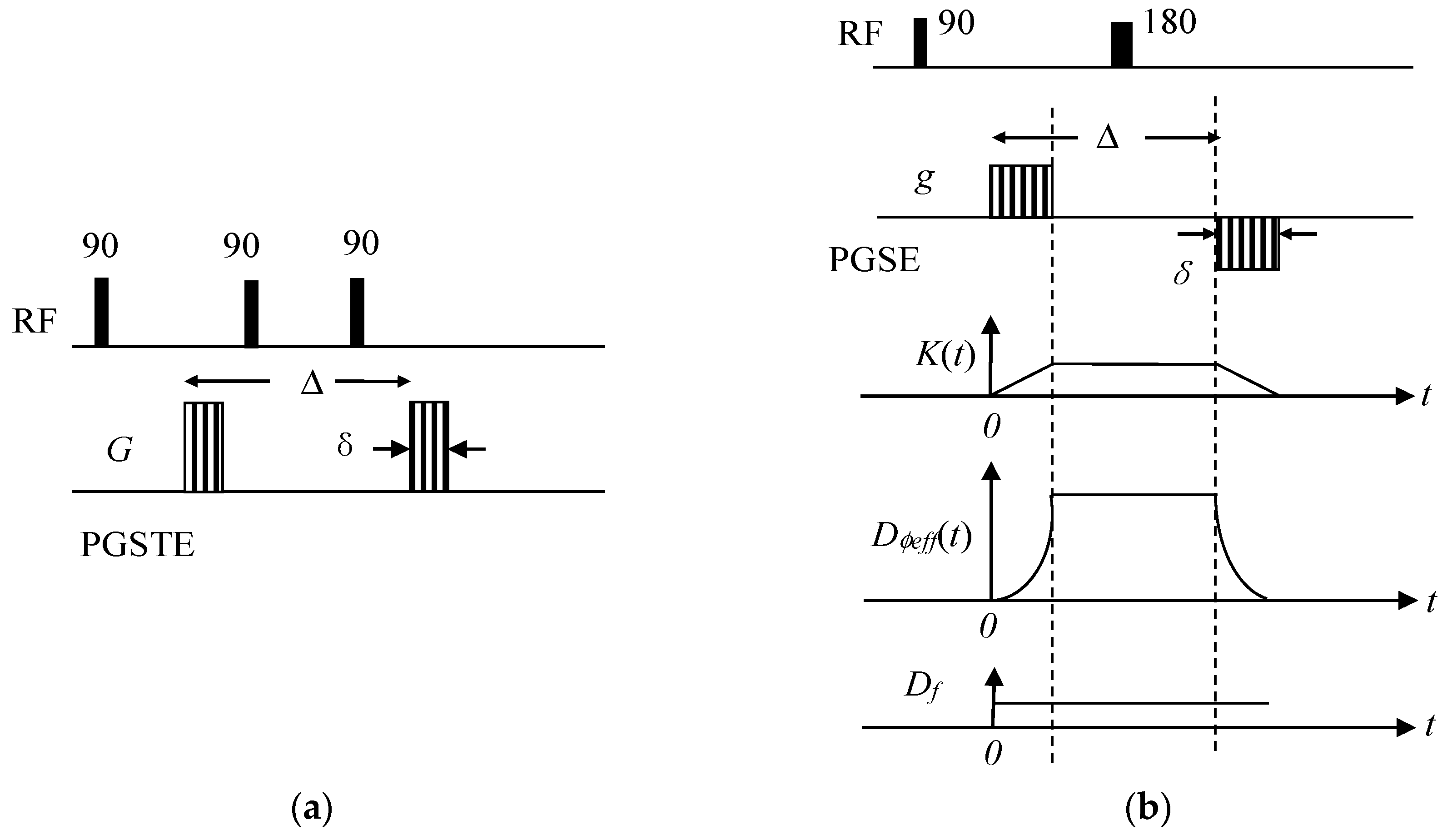
Second, the PFG signal attenuation for general anomalous diffusion can be obtained. The same equation as Equation (17) and its solution have been obtained by the modified Bloch equation method in [30]. According to [30], Equations (12) or (17) can be written equivalently as

$$S(t)={\displaystyle \sum _{k=0}^{m-1}{S}^{(k)}(0^{+})\frac{t^k}{k!}+J^{\alpha }\left(a(t)S(t)\right)},m-1<\alpha <m$$

(20)

where

$$a(t)=-K^{\beta }(t)D_f=\{\begin{array}{c}-{\left(\gamma gt\right)}^{\beta }{D}_f,0<t\le \delta \\ -{\left(\gamma g\delta \right)}^{\beta }{D}_f,\delta <t\le \Delta \\ -{\left(\gamma g\right)}^{\beta }{(\Delta +\delta -t)}^{\beta }{D}_f,\Delta <t\le \Delta +\delta .\end{array}$$

(21)

Based on the Adomian decomposition method [35,36,37,38,39], the solution of Equation (20) is [30,31]

$$S(t)={\displaystyle \sum _{n=0}^{\infty }{S}_n(t)},$$

(22a)

where

$$S_0(t)={\displaystyle \sum _{k=0}^{m-1}{S}^{(k)}(0^{+})\frac{t^k}{k!}},m-1<\alpha <m$$

(22b)

and

$$\begin{array}{ll}{S}_n(t)& =J^{\alpha }\left(a(t)S_{n-1}(t)\right)\\ & =-{\displaystyle \underset{0}{\overset{t}{\int }}\frac{{(t-\tau )}^{\alpha -1}}{\Gamma (\alpha )}{D}_f{K}^{\beta }(\tau )S_{n-1}(\tau )d\tau }\\ & =-{\displaystyle \underset{0}{\overset{t}{\int }}\frac{D_f{K}^{\beta }(\tau )S_{n-1}(\tau )d{(t-\tau )}^{\alpha }}{\alpha \Gamma (\alpha )}}.\end{array}$$

(22c)

In PGSE or PGSTE experiments, the time t can be separated into three periods: $0<t\le \delta$, $\delta <t\le \Delta$, and $\Delta <t\le \Delta +\delta$. If the initial condition, $S^{(1)}(0^{+})=0$, is used [31,32,33,34] for free diffusion in a homogeneous sample, we can get the following:

(a) 

PFG signal attenuation under short gradient pulse (SGP) approximation: $\delta$ is short enough and the diffusion inside each gradient pulse can be neglected. We get

$$S(\Delta )={\displaystyle \sum _{n=0}^{\infty }{S}_n(\Delta )}=E_{\alpha ,1}\left(-D_f{K}_{SGP}{}^{\beta }{\Delta }^{\alpha }\right),K_{SGP}=\gamma g\delta ,$$

(23)

where $S_0(\Delta )=1$, and $S_n(\Delta )=\frac{{\left(-D_f{K}_{SGP}{}^{\beta }{\Delta }^{\alpha }\right)}^n}{\Gamma (1+n\alpha )}$. Equation (23) replicates the SGP approximation result obtained in references [18,26,27].

(b) 

Single pulse attenuation: This is an ideal situation—the first gradient pulse is regular, but the second gradient pulse is infinitely narrow and has the purpose of counteracting the first gradient pulse. We get

$$\begin{array}{ll}S(t)& ={\displaystyle \sum _{n=0}^{\infty }{S}_n(t)}=1+{\displaystyle \sum _{n=1}^{\infty }{\left(-D_f{\left(\gamma g\right)}^{\beta }{t}^{\alpha +\beta }\right)}^n{\displaystyle \prod _{k=1}^n\frac{\Gamma (1+(k-1)\alpha +n\beta )}{\Gamma (1+k(\alpha +\beta ))}}}\\ & =E_{\alpha ,1+\beta /\alpha ,\beta /\alpha }\left(-D_f{\left(\gamma g\right)}^{\beta }{t}^{\alpha +\beta }\right),\end{array}$$

(24)

where $S_0(t)=1$, $S_n(t)={\left(-D_f{\left(\gamma g\right)}^{\beta }{t}^{\alpha +\beta }\right)}^n{\displaystyle \prod _{k=1}^n\frac{\Gamma (1+(k-1)\alpha +n\beta )}{\Gamma (1+k(\alpha +\beta ))}},$ and $E_{\alpha ,\eta ,\gamma }(x)={\displaystyle \sum _{n=0}^{\infty }{c}_n{x}^n},c_0=1,c_n={\displaystyle \prod _{k=0}^{n-1}\frac{\Gamma ((k\eta +\gamma )\alpha +1)}{\Gamma ((k\eta +\gamma +1)\alpha +1)}}$ is a Mittag-Leffler-type function [43]. Equation (24) is consistent with the results obtained by the modified Bloch equation proposed in [25].

(c) 

General PFG signal attenuation: The PGSE or PGSTE experiment includes three periods: $0<t_1\le \delta$, $\delta <t_2\le \Delta$, and $\Delta <t_3\le \Delta +\delta$. The integration in Equation (22c) during these three periods is tedious, but can be calculated with computer assistance. Nevertheless, we can get the first and second terms of Equation (22a) as the following:

$$S_0(t)=1$$

(25a)

$$\begin{array}{l}{S}_1(t)=J^{\alpha }\left(a(t)S_0(t)\right)=-{\displaystyle \underset{0}{\overset{t}{\int }}\frac{{(t-\tau )}^{\alpha -1}}{\Gamma (\alpha )}{D}_f{K}^{\beta }(\tau )d\tau }=-\frac{D_f{\left(\gamma g\right)}^{\beta }}{\Gamma (1+\alpha )}\times \\ \{\begin{array}{l}\alpha t^{\alpha +\beta }B(\beta +1,\alpha ),0<t\le \delta \\ \alpha t^{\alpha +\beta }\left[B(\beta +1,\alpha )-B(\frac{\delta }{t};\beta +1,\alpha )\right]-{\delta }^{\beta }{(t-\delta )}^{\alpha },\delta <t\le \Delta \\ \left\{\alpha t^{\alpha +\beta }\left[B(\beta +1,\alpha )-B(\frac{\delta }{t};\beta +1,\alpha )\right]-{\delta }^{\beta }\left[{(t-\delta )}^{\alpha }-{(t-\Delta )}^{\alpha }\right]\right\}-,\Delta <t\le \Delta +\delta \\ {\displaystyle {\int }_{\Delta }^t\alpha {(t-\tau )}^{\alpha -1}{(\Delta +\delta -t)}^{\beta }d\tau }\end{array}\end{array}$$

(25b)

where B(x,y) and B(a;x,y) are the Beta function and incomplete Beta function, respectively. When $t=\Delta +\delta$, Equation (25b) gives

$$\begin{array}{l}{S}_1(\Delta +\delta )=J^{\alpha }\left(a(t)S_0(t)\right)\\ =-{\displaystyle \underset{0}{\overset{\Delta +\delta }{\int }}\frac{{(\Delta +\delta -\tau )}^{\alpha -1}}{\Gamma (\alpha )}{D}_f{K}^{\beta }(\tau )d\tau }\\ =-\frac{D_f{\left(\gamma g\right)}^{\beta }}{\Gamma (1+\alpha )}\left\{\alpha {(\Delta +\delta )}^{\alpha +\beta }\left[B(\beta +1,\alpha )-B(\frac{\delta }{\Delta +\delta };\beta +1,\alpha )\right]+{\delta }^{\beta }\left({\Delta }^{\alpha }-{\delta }^{\alpha }\right)+\frac{\alpha {\delta }^{\alpha +\beta }}{\alpha +\beta }\right\}.\end{array}$$

(26)

Equation (26) agrees with the signal attenuation expression $S(t)=E_{\alpha ,1}\left(-{\displaystyle {\int }_0^t{D}_f{K}^{\beta }(t^{\prime })d{t^{\prime }}^{\alpha }}\right)$ obtained by the instantaneous signal attenuation method [26]. At small signal attenuation, $S(t)=E_{\alpha ,1}\left(-{\displaystyle {\int }_0^t{D}_f{K}^{\beta }(t^{\prime })d{t^{\prime }}^{\alpha }}\right)$ can be approximately expanded as

$$\begin{array}{l}S(t)=E_{\alpha ,1}\left(-{\displaystyle {\int }_0^t{D}_f{K}^{\beta }(t^{\prime })d{t^{\prime }}^{\alpha }}\right)\\ \approx 1-\frac{D_f{\left(\gamma g\right)}^{\beta }}{\Gamma (1+\alpha )}\left\{\alpha {(\Delta +\delta )}^{\alpha +\beta }\left[B(\alpha ,\beta +1)-B(\frac{\Delta }{\Delta +\delta };\alpha ,\beta +1)\right]+{\delta }^{\beta }\left({\Delta }^{\alpha }-{\delta }^{\alpha }\right)+\frac{\alpha {\delta }^{\alpha +\beta }}{\alpha +\beta }\right\}.\end{array}$$

(27)

Equation (27) is the same as that given by the combination of Equations (25a) and (26) (note that $B(x,y)=B(y,x)$ and $B(a;x,y)=B(1-a;y,x)$); however, at large signal attenuation, $E_{\alpha ,1}\left(-{\displaystyle {\int }_0^t{D}_f{K}^{\beta }(t^{\prime })d{t^{\prime }}^{\alpha }}\right)$ may deviate from the combination of Equations (25a) and (26) as the higher-order terms in the expansion cannot be omitted. This agreement can be explained by the following: in typical PGSE or PGSTE experiments, both the gradient intensity and pulse length of the dephasing pulse and the rephrasing pulse are identical, $\left|g_1\right|=\left|g_2\right|$ and ${\delta }_1={\delta }_2$; thus, $K(\Delta +\delta -\tau )=K(\tau )$, which results in

$$\begin{array}{l}-{\displaystyle \underset{0}{\overset{\Delta +\delta }{\int }}\frac{{(\Delta +\delta -\tau )}^{\alpha -1}}{\Gamma (\alpha )}{D}_f{K}^{\beta }(\tau )d\tau }\stackrel{{\tau }^{\prime }=\Delta +\delta -\tau }{\to }=-{\displaystyle \underset{0}{\overset{\Delta +\delta }{\int }}\frac{{{\tau }^{\prime }}^{\alpha -1}}{\Gamma (\alpha )}{D}_f{K}^{\beta }(\Delta +\delta -{\tau }^{\prime })d{\tau }^{\prime }}\\ \stackrel{K(\Delta +\delta -{\tau }^{\prime })=K({\tau }^{\prime })}{\to }-{\displaystyle \underset{0}{\overset{\Delta +\delta }{\int }}\frac{{{\tau }^{\prime }}^{\alpha -1}}{\Gamma (\alpha )}{D}_f{K}^{\beta }({\tau }^{\prime })d{\tau }^{\prime }}.\end{array}$$

(28)

When $0<\alpha \le 2,\beta =2$, the general anomalous diffusion reduces to time-fractional diffusion and Equation (25b) can be further calculated as

$$\begin{array}{l}{S}_1(\Delta +\delta )=-\frac{D_f{\left(\gamma g\right)}^2}{\Gamma (1+\alpha )}\times \\ \left\{\frac{\alpha {\delta }^{\alpha +2}}{\alpha +2}+{\delta }^2\left({\Delta }^{\alpha }-{\delta }^{\alpha }\right)+\frac{2}{(\alpha +1)(\alpha +2)}\left[{\left(\Delta +\delta \right)}^{2+\alpha }-{\Delta }^{2+\alpha }\right]-\frac{2}{\alpha +1}{\Delta }^{1+\alpha }\delta -{\Delta }^{\alpha }{\delta }^2\right\}.\end{array}$$

(29)

When $\alpha =1,0<\beta \le 2$, the general anomalous diffusion reduces to space-fractional diffusion. Equation (22) reduces to $S(t)=\exp \left(-{\displaystyle {\int }_0^t{D}_f{K}^{\beta }(t^{\prime })d{t}^{\prime }}\right)$, which is the same as that obtained by [18,26,30,31].

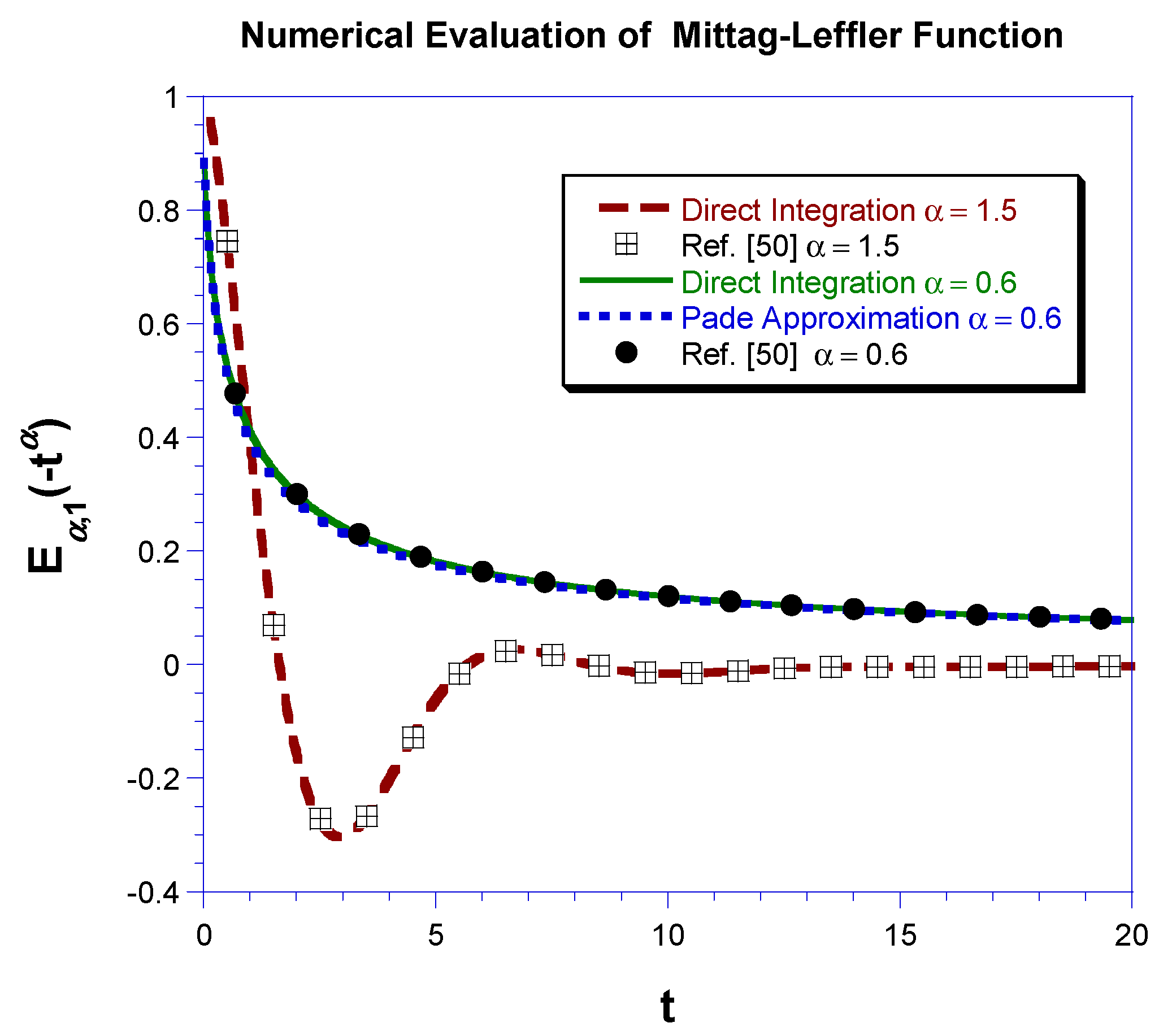
2.4. Numerical Evaluation of Mittag-Leffler Function-Based PFG Signal Attenuation by the Direct Integration Method

Although the Adomian decomposition method can be used to numerically evaluate the PFG signal attenuation, its calculation speed is slow and it could cause overflow at large signal attenuation. References [30,31,44] proposed an alternative method: a direct integration method that can give the same numerical results, but with a much faster speed and without overflow. From Equation (20), if we set ${\displaystyle \sum _{k=0}^{m-1}{S}^{(k)}(0^{+})\frac{t^k}{k!}}=1$, we have [44]

$$S(t)=1-{\displaystyle \underset{0}{\overset{t}{\int }}\frac{{(t-\tau )}^{\alpha -1}}{\Gamma (\alpha )}G(\tau )S(\tau )d\tau },$$

(30)

where $G(t)=K^{\beta }(t)D_f$. If we denote $E_{\alpha ,1,G(t)}(-t)=S(t)$, Equation (30) can be further written as [44]

$$E_{\alpha ,1,G(t)}(-t)=1-{\displaystyle \underset{0}{\overset{t}{\int }}\frac{{(t-\tau )}^{\alpha -1}}{\Gamma (\alpha )}G(\tau )E_{\alpha ,1,G(t)}(-\tau )d\tau }.$$

(31a)

When $G(t)=1$, $E_{\alpha ,1,G(t)}(-t)=E_{\alpha ,1}(-t^{\alpha })$, which is a Mittag-Leffler function (MLF); when $G(t)=c,c>0$, $E_{\alpha ,1,G(t)}(-t)=E_{\alpha ,1}(-c{t}^{\alpha })$. Hence, we have [44]

$$E_{\alpha ,1}(-t^{\alpha })=1-{\displaystyle \underset{0}{\overset{t}{\int }}\frac{{(t-\tau )}^{\alpha -1}}{\Gamma (\alpha )}{E}_{\alpha ,1}(-{\tau }^{\alpha })d\tau },$$

(31b)

$$E_{\alpha ,1}(-c{t}^{\alpha })=1-{\displaystyle \underset{0}{\overset{t}{\int }}\frac{{(t-\tau )}^{\alpha -1}}{\Gamma (\alpha )}c{E}_{\alpha ,1}(-c{\tau }^{\alpha })d\tau }.$$

(31c)

Equation (30) can be rewritten in a discrete form as [44]

$$S(t_j)=1-{\displaystyle \sum _{k=1}^{j}a(t_k)S(t_{k-1})\left[{(t_j-t_{k-1})}^{\alpha }-{(t_j-t_k)}^{\alpha }\right]}/\Gamma (1+\alpha ),$$

(32)

where $t_j={\displaystyle \sum _{k=1}^j\Delta t_k}$. Based on Equation (32), the PFG signal attenuations $S(t_1)$, $S(t_2)$,…, $S(t_n)$ can be calculated step by step starting from $S(t_1)$ through to $S(t_n)$. Similarly, the Mittag-Leffler-type function and its derivative can be numerically evaluated by [44]

$$E_{\alpha ,1,G(t)}(-t_j)=1-{\displaystyle \sum _{k=1}^{j}G(t_k)E_{\alpha ,1,G(t)}(-t_{k-1})\left[{(t_j-t_{k-1})}^{\alpha }-{(t_j-t_k)}^{\alpha }\right]}/\Gamma (1+\alpha ),$$

(33)

$$E_{\alpha ,1,G(t)}^{\prime }(-t_j)=\frac{E_{\alpha ,1,G(t)}(-t_j)-E_{\alpha ,1,G(t)}(-t_{j-1})}{\Delta t_j}.$$

(34)

This method is simple, and there is no overflow issue in the calculation.

3. Continuous-Time Random Walk (CTRW) in a Lattice Model

Random walk simulation is a powerful numerical method that employs a stochastic jump process to model normal and anomalous diffusion in physics, chemistry, biology, and many other disciplines. It can be used to simulate the PFG signal attenuation in mathematically tractable or intractable systems. In this paper, the continuous-time random walk (CTRW) simulation method developed in [26] is used to verify the theoretical results; it is based on two models: the CTRW model [45] and the Lattice model [46,47]. In the simulation, a sequence of independent random waiting time and jump length combinations ($\Delta t_1$, $\Delta {\xi }_1$), ($\Delta t_2$, $\Delta {\xi }_2$), ($\Delta t_3$, $\Delta {\xi }_3$),…, ($\Delta t_n$, $\Delta {\xi }_n$) is produced by the computer program. The individual waiting time $\Delta t$ and jump length $\Delta \xi$ are given according to [26] by the following expressions:

$$\Delta t=-{\eta }_t\log U{\left(\frac{\sin (\alpha \pi )}{\tan (\alpha \pi V)}-\cos (\alpha \pi )\right)}^{\frac{1}{\alpha }}$$

(35)

and

$$\Delta \xi ={\eta }_z{\left(\frac{-\log U\cos (\mathsf{\Phi })}{\cos ((1-\beta )\mathsf{\Phi })}\right)}^{1-\frac{1}{\beta }}\frac{\sin (\beta \mathsf{\Phi })}{\cos (\mathsf{\Phi })}$$

(36)

where ${\eta }_t$ and ${\eta }_z$ are scale constants, $\mathsf{\Phi }=\pi (V-1/2)$, and $U,V\in (0,1)$ are two independent random numbers. The CTRW simulation based on the above waiting time and jump length satisfies the time–space fractional diffusion equation under the diffusive limit, providing a simple way to simulate anomalous diffusion in various research areas, such as physics and economics [45].

Although continuous waiting time and jump length are used in the simulation, the accumulating spin phase associated with the diffusion path is recorded in a discrete manner. Such a discrete phase recording manner is convenient and reasonable. The simulation can be viewed as a numerical PFG experiment, whose observables such as phase can be observed in a discrete time selected by an experiment observer; the observing or recording manner will not affect the fundamental numerical experiment process, namely the production of the continuous random walk sequence ($\Delta t_1$, $\Delta {\xi }_1$), ($\Delta t_2$, $\Delta {\xi }_2$), ($\Delta t_3$, $\Delta {\xi }_3$) ,…, ($\Delta t_n$, $\Delta {\xi }_n$). The spin phase was recorded by the lattice model developed in [46,47], which has been applied to simulate PFG diffusion in polymer systems [48]. The spin phase in the simulation is

$$\varphi (t_{j^{\prime }}^{\prime })={\displaystyle \sum _{j=1}^l\gamma g(t_j)\xi (t_j)\Delta t_j+\gamma g(t_{j^{\prime }}^{\prime })\xi (t_{l+1})(t_{j^{\prime }}^{\prime }-t_l)},t_l\le t_{j^{\prime }}^{\prime }\le t_{l+1}$$

(37)

where $t_l={\displaystyle \sum _{j=1}^l\Delta t_j}$, $\xi (t_l)={\displaystyle \sum _{j=1}^l\Delta {\xi }_j},$ and $t_{j^{\prime }}^{\prime }$ is the discrete record time, which takes place between the lth and (l + 1)th steps of the random walk. The second term $\gamma g(t_{j^{\prime }}^{\prime })\xi (t_{l+1})(t_{j^{\prime }}^{\prime }-t_l)$ on the right-hand side of Equation (37) corresponds to the partial phase evolution of the (l + 1)th jump step that needs to be recorded at the time $t_{j^{\prime }}^{\prime }$. The PFG signal attenuation in the simulation can be obtained by averaging over all the walkers in the simulation [26,47,48]:

$$S(t)=\langle \cos \left[{\varphi }_i(t)\right]\rangle =\frac{1}{N_{walks}}{\displaystyle \sum _{i=1}^{N_{walks}}\cos \left[{\varphi }_i(t)\right]},$$

(38)

where $N_{walks}$ is the total number of walks. The total number of walks used in each simulation is 1,000,000.

Because the CTRW model proposed in [25] is only for subdiffusion, the simulation here is limited to the subdiffusion. Please refer to references [26,30,45,46,47,48] for more detailed information.

4. Results and Discussion

This paper uses two different methods to describe PFG anomalous diffusion: the EPSDE method [18] and the method of observing the signal intensity at the origin. The major results in this paper are summarized in

Table 1. Comparison of pulsed-field gradient (PFG) anomalous diffusion results by the effective phase-shift diffusion method, the observing the signal intensity at the origin method and other methods.

Virtual Phase-Space Diffusion	Real-Space Spin Diffusion
Effective phase-shift diffusion equation [18]	Observing the signal intensity at the origin
Diffusion equations:
${}_t{D}_{*}^{\alpha }P\left(\varphi ,t\right)=K^{\beta }(t)D_f\frac{{\partial }^{\beta }}{\partial {\left|\varphi \right|}^{\beta }}P\left(\varphi ,t\right)$ [18]	${}_t{D}_{*}^{\alpha }{M}_{xy}\left(z,t\right)=D_f\frac{{\partial }^{\beta }}{\partial {\left|z\right|}^{\beta }}{M}_{xy}\left(z,t\right)$ [32]
Solving methods:
Fourier transform	Substitute $M_{xy}\left(z,t\right)=S(t)\exp (-iK(t)\cdot z)$ into equation
PFG signal attenuation equation*:
${}_t{D}_{*}^{\alpha }S\left(t\right)=-D_f{K}^{\beta }(t)S\left(t\right)$,
or equivalently $S(t)={\displaystyle \sum _{k=0}^{m-1}{S}^{(k)}(0^{+})\frac{t^k}{k!}+J^{\alpha }\left(a(t)S(t)\right)},m-1<\alpha <m$
PFG signal attenuation expression by the Adomian decomposition method [30,31]*:
$S(t)={\displaystyle \sum _{n=0}^{\infty }{S}_n(t)},$
where $S_0(t)={\displaystyle \sum _{k=0}^{m-1}{S}^{(k)}(0^{+})\frac{t^k}{k!}},m-1<\alpha <m$, and $S_n(t)=-{\displaystyle \underset{0}{\overset{t}{\int }}\frac{{(t-\tau )}^{\alpha -1}{D}_f{K}^{\beta }(\tau )S_{n-1}(\tau )d\tau }{\Gamma (\alpha )}}$
Under short gradient pulse (SGP) approximation: $S(\Delta )=E_{\alpha ,1}\left(-D_f{K}_{SGP}{}^{\beta }{\Delta }^{\alpha }\right),K_{SGP}=\gamma g\delta$
At small attenuation:	$S(t)\approx E_{\alpha ,1}\left(-{\displaystyle {\int }_0^t{D}_f{K}^{\beta }(t^{\prime })d{t^{\prime }}^{\alpha }}\right)$
Other methods:
(1) $S(t)=E_{\alpha ,1+\beta /\alpha ,\beta /\alpha }\left(-{\gamma }^{\beta }{t}^{\alpha +\beta }{{\displaystyle \underset{g}{\int }\left|g\cdot y\right|}}^{\beta }m(dy)\right)$ [25]
(2) $E_{\alpha ,1}\left[-i\gamma g\tau {\left(t/\tau \right)}^{\alpha }\right]\exp \left[-B{\left(t/\tau \right)}^{\alpha }\right],B=\frac{2\Gamma (2-\alpha )D_f{\gamma }^2{g}^2{\tau }^3}{3{\alpha }^2\Gamma (2-\alpha )}$ [17]
(3) $S(t)\approx E_{\alpha ,1}\left(-{\displaystyle {\int }_0^t{D}_f{K}^{\beta }(t^{\prime })d{t^{\prime }}^{\alpha }}\right)$ [26]
(4) $S(\Delta )=E_{\alpha ,1}\left(-D_f{K}_{SGP}{}^{\beta }{\Delta }^{\alpha }\right),K_{SGP}=\gamma g\delta$ [18,26,27]

* The PFG signal attenuation equation and expression obtained in this paper are the same as that obtained by the integral modified Bloch equation method [30].

. The EPSDE method [18] uses an effective phase diffusion process to describe the phase evolution, while observing the signal intensity at the origin only monitors the real-space signal amplitude change at the origin where the phase of the magnetization remains constant. Each of these two approaches has its unique advantages. The EPSDE method can directly obtain the phase distribution, which greatly simplifies PFG diffusion analysis [18]; in contrast, the traditional methods often need to get the real-space spin particle probability distribution first, which is then used to obtain the phase distribution. The ultra-simple method of observing the signal intensity at the origin obtains the signal attenuation equation by substituting the magnetization $M_{xy}\left(z,t\right)=S(t)\exp (-iK(t)\cdot z)$ directly into the diffusion equation and using the phase property $\exp (-iK(t)\cdot z)=1$ and $i\gamma gz=0$ at the origin. These two approaches view the spin evolution process from two different spaces—the real space and the phase space—providing a clear picture of spin dynamics in PFG diffusion experiments.

These two methods agree with each other. They get the same PFG signal attenuation Equation (11) or (16), which can be solved by the Adomian decomposition method. The solution gives PFG signal attenuation expressions (21a)–(21c), which include the FGPW effect. Understanding the FGPW effect is important as clinical MRI applications often use a long gradient pulse. Additionally, using long gradient pulses allows researchers to monitor slower diffusion in polymer or biological systems where the molecules or ions often diffuse slowly. The consistent results from two different methods help us better understand the FGPW effect.

Additionally, the two methods agree with other methods. First, the PFG signal attenuation Equation (17) obtained here is the same as that obtained by the integral modified Bloch equation method [30,31]. Second, the results agree with the CTRW simulation as shown in Figure 2. In Figure 2a, the fractional diffusion constant $D_f$ = 6.6 × 10⁻¹¹ m^β/s^α was obtained from fitting the curve of mean square displacement versus t by equation $\langle {\left|z\right|}^{\beta }\rangle =2D_f{t}^{\alpha }/\Gamma (1+\alpha )$. Figure 2b shows the PFG signal attenuation of anomalous diffusion obtained by Equations (22a)–(22c) based on the Adomian decomposition method, Equation (32) based on the direct integration method, and the CTRW simulation. Other parameters used in Figure 2 are $\alpha =0.5,\beta =2$, g = 0.1 T/m, $\Delta -\delta$ equaling 0 ms, 20 ms. Interested readers can refer to [30] for additional comparisons between the theoretical prediction and the CTRW simulation. Third, the PFG signal attenuation expressions (22a)–(22c) are also consistent with those obtained by various approximation methods such as the non-Gaussian phase distribution (nGPD) method [27] and the instantaneous signal attenuation method [26]. The same SGP approximation results, Equation (23), can be obtained by all these five different methods: the EPSDE method [18], the instantaneous signal attenuation method [26], the nGPD method [27], the method to observe the signal intensity at the origin, and the modified Bloch equation method [30]. Moreover, Equation (27), $S(t)\approx E_{\alpha ,1}\left(-{\displaystyle {\int }_0^t{D}_f{K}^{\beta }(t^{\prime })d{t^{\prime }}^{\alpha }}\right)$, can be approximately obtained in this paper; this agrees with the result obtained from the instantaneous signal attenuation method [26].

The numerical evaluation of PFG signal attenuation by Equation (20) or (30) can be conveniently performed by the direct integration method. Figure 2b shows that the results of the direct integration method agree with those obtained from the Adomian decomposition method. Compared to the Adomian decomposition method, the computing speed of the direct integration method improves by orders of magnitudes. The speed improvement is because in the direct integration method, each $S(t_j)$ in Equation (32) is only a single time integration, while in the Adomian decomposition method, $S(t_j)={\displaystyle \sum _{n=0}^{\infty }{S}_n(t_j)}$ is a superposition of many terms of time integration. Additionally, from Equations (33) and (34), the direct integration method can be used to calculate Mittag-Leffler-type functions and their derivatives. Figure 3 shows that the MLF calculated from the direct integration method agrees with that calculated by other methods in [49,50]. The Pade approximation method in [50] is only for subdiffusion. Because the direct integration method does not cause overflow, it can be a useful method for calculating Mittag-Leffler-type functions. The Fortran code for MLF calculation by the direct integration method can be obtained from the following link: https://github.com/GLin2017/Mittag-Leffler-function-calculated-by-Direct-Integration. Matlab code for calculating the MLF function by other methods to a desired accuracy can be found at www.mathworks.com/matlabcentral/fileexchange/8738-mittag-leffer-function, 2005. This direct integration method will be a great help to the application of current theoretical results to PFG anomalous diffusion in NMR and MRI.

In the current results, only PFG anomalous diffusion of single quantum coherence is considered. The results here can be easily extended to handle PFG anomalous diffusion of intramolecular MQC [27,40]. As the gradient field-induced phase evolution of an n-order intramolecular MQC is n times faster than the corresponding single quantum coherence, the PFG signal attenuation of intramolecular MQC is the same as that of single quantum coherence with an effective gradient intensity ng [42]. Therefore, for intramolecular MQC in PGSE or PGSTE experiments, the PFG signal attenuation equation is

$$S(t)={\displaystyle \sum _{k=0}^{m-1}{S}^{(k)}(0^{+})\frac{t^k}{k!}+J^{\alpha }\left(a_{MQC}(t)S(t)\right)},m-1<\alpha <m,$$

(39)

where

$$a_{MQC}(t)=-K_{MQC}{}^{\beta }(t)D_f=\{\begin{array}{c}-n^{\beta }{\left(\gamma gt\right)}^{\beta }{D}_f,0<t\le \delta \\ -n^{\beta }{\left(\gamma g\delta \right)}^{\beta }{D}_f,\delta <t\le \Delta \\ -n^{\beta }{\left(\gamma g\right)}^{\beta }{(\Delta +\delta -t)}^{\beta }{D}_f,\Delta <t\le \Delta +\delta .\end{array}$$

(40)

From Equation (40), it is obvious that the $a_{MQC}(t)$ in the MQC equals $n^{\beta }a(t)$.

This paper only considers the spin self-diffusion that can be described by the time–space fractional diffusion equation based on the fractional derivative. In general, the two methods used in this paper can be applied to other types of anomalous diffusions such as that described by the time–space diffusion equation based on the fractal derivative [51], etc. Additionally, only the symmetric anomalous diffusion in homogeneous spin systems is studied here. In real applications, the anomalous diffusion can take place in complicated systems such as inhomogeneous systems, restricted geometries [28], anisotropic systems [44], nonsymmetric systems, etc. Additionally, the gradient field may be nonlinear [52]. The current methods may face challenges in these complicated situations, which reminds us that much effort is required for the study of PFG anomalous diffusion.

References

1. Wyss, W. The fractional diffusion equation. J. Math. Phys. 1986, 27, 2782–2785. [Google Scholar] [CrossRef]
2. Metzler, R.; Klafter, J. The random walk’s guide to anomalous diffusion: A fractional dynamics approach. Phys. Rep. 2000, 339, 1–77. [Google Scholar] [CrossRef]
3. Sokolov, I.M. Models of anomalous diffusion in crowded environments. Soft Matter 2012, 8, 9043–9052. [Google Scholar] [CrossRef]
4. Povstenko, Y. Linear Fractional Diffusion-Wave Equation for Scientists and Engineers; Birkhäuser: New York, NY, USA, 2015. [Google Scholar]
5. Köpf, M.; Corinth, C.; Haferkamp, O.; Nonnenmacher, T.F. Anomalous diffusion of water in biological tissues. Biophys. J. 1996, 70, 2950–2958. [Google Scholar] [CrossRef]
6. Saichev, A.I.; Zaslavsky, G.M. Fractional kinetic equations: Solutions and applications. Chaos 1997, 7, 753–764. [Google Scholar] [CrossRef] [PubMed]
7. Lindsey, C.P.; Patterson, G.D. Detailed comparison of the Williams–Watts and Cole-Davidson functions. J. Chem. Phys. 1980, 73, 3348–3357. [Google Scholar] [CrossRef]
8. Kaplan, J.I.; Garroway, A.N. Homogeneous and inhomogeneous distributions of correlation times. Lineshapes for chemical exchange. J. Magn. Reson. 1982, 49, 464–475. [Google Scholar] [CrossRef]
9. Hahn, E.L. Spin echoes. Phys. Rev. 1950, 80, 580–594. [Google Scholar] [CrossRef]
10. Torrey, H.C. Bloch Equations with Diffusion Terms. Phys. Rev. 1956, 104, 563–565. [Google Scholar] [CrossRef]
11. McCall, D.W.; Douglass, D.C.; Anderson, E.W. Self-diffusion studies by means of nuclear magnetic resonance spin-echo techniques. Ber. Bunsenges. Phys. Chem. 1963, 67, 336–340. [Google Scholar] [CrossRef]
12. Stejskal, E.O.; Tanner, J.E. Spin diffusion measurements: Spin echoes in the presence of a time-dependent field gradient. J. Chem. Phys. 1965, 42, 288–292. [Google Scholar] [CrossRef]
13. Price, W.S. Pulsed-field gradient nuclear magnetic resonance as a tool for studying translational diffusion: Part 1. Basic theory. Concepts Magn. Reson. 1997, 9, 299–336. [Google Scholar] [CrossRef]
14. Price, W.S. NMR Studies of Translational Motion: Principles and Applications; Cambridge University Press: Cambridge, UK, 2009. [Google Scholar]
15. Callaghan, P. Translational Dynamics and Magnetic Resonance: Principles of Pulsed Gradient Spin Echo NMR; Oxford University Press: Oxford, UK, 2011. [Google Scholar]
16. McRobbie, D.W.; Moore, E.A.; Graves, M.J.; Prince, M.R. MRI from Picture to Proton, 2nd ed.; Cambridge University Press: Cambridge, UK, 2007; p. 338. [Google Scholar]
17. Magin, R.L.; Abdullah, O.; Baleanu, D.; Zhou, X.J. Anomalous diffusion expressed through fractional order differential operators in the Bloch–Torrey equation. J. Magn. Reson. 2008, 190, 255–270. [Google Scholar] [CrossRef] [PubMed]
18. Lin, G. An effective phase shift diffusion equation method for analysis of PFG normal and fractional diffusions. J. Magn. Reson. 2015, 259, 232–240. [Google Scholar] [CrossRef] [PubMed]
19. Kärger, J.; Pfeifer, H.; Vojta, G. Time correlation during anomalous diffusion in fractal systems and signal attenuation in NMR field-gradient spectroscopy. Phys. Rev. A 1988, 37, 4514–4517. [Google Scholar] [CrossRef]
20. Kimmich, R. NMR: Tomography, Diffusometry, Relaxometry; Springer: Heidelberg, Germany, 1997. [Google Scholar]
21. Fatkullin, N.; Kimmich, R. Theory of field-gradient NMR diffusometry of polymer segment displacements in the tube-reptation model. Phys. Rev. E 1995, 52, 3273–3276. [Google Scholar] [CrossRef]
22. Bennett, K.M.; Schmainda, K.M.; Bennett, R.T.; Rowe, D.B.; Lu, H.; Hyde, J.S. Characterization of continuously distributed cortical water diffusion rates with a stretched-exponential model. Magn. Reson. Med. 2003, 50, 727–734. [Google Scholar] [CrossRef] [PubMed]
23. Bennett, K.M.; Hyde, J.S.; Schmainda, K.M. Water diffusion heterogeneity index in the human brain is insensitive to the orientation of applied magnetic field gradients. Magn. Reson. Med. 2006, 56, 235–239. [Google Scholar] [CrossRef] [PubMed]
24. Klafter, J.; Sokolov, I.M. First Step in Random Walks. From Tools to Applications; Oxford University Press: New York, NY, USA, 2011. [Google Scholar]
25. Hanyga, A.; Seredyńska, M. Anisotropy in high-resolution diffusion-weighted MRI and anomalous diffusion. J. Magn. Reson. 2012, 220, 85–93. [Google Scholar] [CrossRef] [PubMed]
26. Lin, G. Instantaneous signal attenuation method for analysis of PFG fractional diffusions. J. Magn. Reson. 2016, 269, 36–49. [Google Scholar] [CrossRef] [PubMed]
27. Lin, G. Analyzing signal attenuation in PFG anomalous diffusion via a non-gaussian phase distribution approximation approach by fractional derivatives. J. Chem. Phys. 2016, 145, 194202. [Google Scholar] [CrossRef] [PubMed]
28. Lin, G.; Zheng, S.; Liao, X. Signal attenuation of PFG restricted anomalous diffusions in plate, sphere, and cylinder. J. Magn. Reson. 2016, 272, 25–36. [Google Scholar] [CrossRef] [PubMed]
29. Damion, R.A.; Packer, K.J. Predictions for pulsed-field-gradient NMR experiments of diffusion in fractal spaces. Proc. Math. Phys. Eng. Sci. 1997, 453, 205–211. [Google Scholar] [CrossRef]
30. Lin, G. The exact PFG signal attenuation expression based on a fractional integral modified-Bloch equation. arXiv, 2017; arXiv:1706.02026. [Google Scholar]
31. Lin, G. Fractional differential and fractional integral modified-Bloch equations for PFG anomalous diffusion and their general solutions. arXiv, 2017; arXiv:1702.07116. [Google Scholar]
32. Mainardi, F.; Luchko, Y.; Pagnini, G. The fundamental solution of the space-time-fractional diffusion equation. Fract. Calc. Appl. Anal. 2001, 4, 153–192. [Google Scholar]
33. Gorenflo, R.; Mainardi, F. Fractional Diffusion Processes: Probability Distributions and Continuous Time Random Walk. In Processes with Long-Range Correlations. Theory and Applications; Rangarajan, G., Ding, M., Eds.; Lecture Notes in Physics, No. 621; Springer: Berlin, Germany, 2003; pp. 148–166. [Google Scholar]
34. Balescu, R. V-Langevin equations, continuous time random walks and fractional diffusion. Chaos Solitons Fract. 2007, 34, 62–80. [Google Scholar] [CrossRef]
35. Mittal, R.C.; Nigam, R. Solution of fractional integro-differential equations by Adomian decomposition method. Int. J. Appl. Math. Mech. 2008, 4, 87–94. [Google Scholar]
36. Adomian, G. Solving Frontier Problems of Physics: The Decomposition Method; Kluwer Academic: Dordrecht, The Netherlands, 1994. [Google Scholar]
37. Adomian, G.; Rach, R. Inversion of nonlinear stochastic operators. J. Math. Anal. Appl. 1983, 91, 39–46. [Google Scholar] [CrossRef]
38. Adomian, G.; Rach, R. On the solution of algebraic equations by the decomposition method. J. Math. Anal. Appl. 1985, 105, 141–166. [Google Scholar] [CrossRef]
39. Duan, J.-S.; Rach, R.; Baleanu, D.; Wazwaz, A.-M. A review of the Adomian decomposition method and its applications to fractional differential equations. Commun. Fract. Calc. 2012, 3, 73–99. [Google Scholar]
40. Grinberg, F.; Farrher, E.; Ciobanu, L.; Geffroy, F.; Le Bihan, D.; Shah, N.J. Non-Gaussian diffusion imaging for enhanced contrast of brain tissue affected by ischemic stroke. PLoS ONE 2014, 9, e89225. [Google Scholar] [CrossRef] [PubMed]
41. Zax, D.; Pines, A. Study of anisotropic diffusion of oriented molecules by multiple quantum spin echoes. J. Chem. Phys. 1983, 78, 6333–6334. [Google Scholar] [CrossRef]
42. Karlicek, R.F., Jr.; Lowe, I.J. A modified pulsed gradient technique for measuring diffusion in the presence of large background gradients. J. Magn. Reson. 1980, 37, 75–91. [Google Scholar] [CrossRef]
43. Kilbas, A.A.; Saigo, M. Solutions of integral equation of Abel–Volterra type. Differ. Integral Equ. 1995, 8, 993–1011. [Google Scholar]
44. Lin, G. General PFG signal attenuation expressions for anisotropic anomalous diffusion by modified-Bloch equations. Physica A 2018. [Google Scholar] [CrossRef]
45. Germano, G.; Politi, M.; Scalas, E.; Schilling, R.L. Stochastic calculus for uncoupled continuous-time random walks. Phys. Rev. E 2009, 79, 066102. [Google Scholar] [CrossRef] [PubMed]
46. Cicerone, M.T.; Wagner, P.A.; Ediger, M.D. Translational diffusion on heterogeneous lattices: A model for dynamics in glass forming materials. J. Phys. Chem. B 1997, 101, 8727–8734. [Google Scholar] [CrossRef]
47. Lin, G.; Zhang, J.; Cao, H.; Jones, A.A. A lattice model for the simulation of diffusion in heterogeneous polymer systems. Simulation of apparent diffusion constants as determined by pulse-field-gradient nuclear magnetic resonance. J. Phys. Chem. B 2003, 107, 6179–6186. [Google Scholar] [CrossRef]
48. Lin, G.; Aucoin, D.; Giotto, M.; Canfield, A.; Wen, W.; Jones, A.A. Lattice model simulation of penetrant diffusion along hexagonally packed rods in a barrier matrix as determined by pulsed-field-gradient nuclear magnetic resonance. Macromolecules 2007, 40, 1521–1528. [Google Scholar] [CrossRef]
49. Gorenflo, R.; Loutchko, J.; Luchko, Y. Computation of the Mittag-Leffler function Eα,β (z) and its derivative. Fract. Calc. Appl. Anal. 2002, 5, 491–518. [Google Scholar]
50. Zeng, C.; Chen, Y. Global Pade approximations of the generalized Mittag-Leffler function and its inverse. Fract. Calc. Appl. Anal. 2015, 18, 1492–1506. [Google Scholar] [CrossRef]
51. Chen, W.; Sun, H.; Zhang, X.; Korošak, D. Anomalous diffusion modeling by fractal and fractional derivatives. Comput. Math. Appl. 2010, 59, 1754–1758. [Google Scholar] [CrossRef]
52. Le Doussal, P.; Sen, P.N. Decay of nuclear magnetization by diffusion in a parabolic magnetic field: An exactly solvable model. Phys. Rev. B 1992, 46, 3465–3485. [Google Scholar] [CrossRef]
Figure 1. (a) Pulsed gradient stimulated echo (PGSTE) pulse sequences; (b) pulsed gradient spin echo (PGSE) pulse sequence. The gradient pulse width is δ , and the diffusion delay is Δ . The time-dependent behavior of wavenumber K ( t ) , diffusion constant D f , and the effective phase diffusion constant D ϕ e f f ( t ) = K β ( t ) D f are also demonstrated below the PGSE pulse sequence.
Mathematics 06 00017 g001
Figure 2. Comparison of the PFG signal attenuation from theoretical predictions with continuous-time random walk (CTRW) simulation: (a) mean square displacement from CTRW simulation; (b) PFG signal attenuation from different methods: the Adomian decomposition method with Equations (22a)–(22c), the direct integration method with Equation (32), and the CTRW simulation. The parameters used are α = 0.5 ,   β = 2 , D f = 6.6 × 10⁻¹¹ mβ/sα, and g = 0.1 T/m.
Mathematics 06 00017 g002
Figure 3. Comparing the Mittag-Leffler function (MLF) calculated by different methods: Equation (33) from the direct integration method, the Pade approximation method [50], and the method used in [49].
Mathematics 06 00017 g003