Critical Domain Problem for the Reaction–Telegraph Equation Model of Population Dynamics

Department of Mathematics, University of Leicester, University Road, Leicester LE1 7RH, UK
*
Author to whom correspondence should be addressed.
Mathematics 2018, 6(4), 59; https://doi.org/10.3390/math6040059
Submission received: 28 February 2018
/
Revised: 5 April 2018
/
Accepted: 13 April 2018
/
Published: 17 April 2018
(This article belongs to the Special Issue Progress in Mathematical Ecology)
Abstract
:A telegraph equation is believed to be an appropriate model of population dynamics as it accounts for the directional persistence of individual animal movement. Being motivated by the problem of habitat fragmentation, which is known to be a major threat to biodiversity that causes species extinction worldwide, we consider the reaction–telegraph equation (i.e., telegraph equation combined with the population growth) on a bounded domain with the goal to establish the conditions of species survival. We first show analytically that, in the case of linear growth, the expression for the domain’s critical size coincides with the critical size of the corresponding reaction–diffusion model. We then consider two biologically relevant cases of nonlinear growth, i.e., the logistic growth and the growth with a strong Allee effect. Using extensive numerical simulations, we show that in both cases the critical domain size of the reaction–telegraph equation is larger than the critical domain size of the reaction–diffusion equation. Finally, we discuss possible modifications of the model in order to enhance the positivity of its solutions.
1. Introduction
Habitat fragmentation due to the climate change and anthropogenic activities is regarded as a major threat to biodiversity worldwide [1]. Understanding the factors affecting species survival in small and fragmented habitats is therefore a problem of high practical importance [2,3,4]. Although being essentially an ecological problem, it can hardly be studied in full by only traditional ecological methods and tools. Replicated ecological experiments under controlled conditions required for an exhaustive empirical study are often impossible for a variety of reasons, e.g., due to high costs, potential damage to the environment, and irreproducibility of the weather conditions and initial species distribution, to name just a few.
Mathematical modelling has long been recognized as an efficient research tool in theoretical ecology that can be used as a supplement and sometimes even a substitute to a field experiment [5,6]. Mathematical models along with computer simulations create a virtual laboratory where hypotheses can be tested and different scenarios can be followed under safe working conditions and at relatively low costs. In particular, the problem of population persistence in small habitats, often referred to as the problem of critical domain, has been studied almost exhaustively in terms of reaction–diffusion models [7,8,9,10,11].
The choice of an adequate model, however, is a subtle issue. Whilst reaction–diffusion models have been used extensively in mathematical ecology for several decades [8,12,13,14,15] helping to make a number of important insights and inferences, they have their limits and their relevance may sometimes become questionable. One point of their criticism is that diffusion (Brownian motion) as a baseline animal movement pattern is not entirely realistic as the diffusively moving ‘animal’ can change its movement direction with a high frequency (i.e., with any two consequent turns infinitely close in time) and choose the new direction uniformly distributed over the circle. However, this is at odds with many observations as well as with common sense [16]: since the body of animals of all species has the front end and the rear end, they are more likely to choose the new movement direction (following re-orientation) close to the movement direction at the preceding moment. The corresponding movement pattern is known as the correlated random walk (CRW) [17] and the corresponding microscopic stochastic process as the telegraph process [18], and their mean-field counterpart is known as a telegraph equation [19,20,21,22,23]:
where is the population density at location x and time t, D is the diffusion coefficient, and is a characteristic time of the microscopic movement that quantifies directional persistence in individual animal movement. The precise meaning of parameter can be slightly different depending on the details of the microscopic model; for instance, in the telegraph movement process, it is the time over which the animal moves without changing its movement direction [18,19,20]. Brownian motion thus corresponds to the limit when Equation (1) turns into the diffusion equation.
Equation (1) describes the evolution of the population density because of animal movement. It does not take into account the contribution of births and deaths. Interestingly, in order to include them into the model, it is not enough to add the ‘reaction’ term (i.e., the population growth rate)—say, —into the right-hand side of Equation (1) (as is done in the case of diffusive animal movement [14]). An accurate account for birth and death events also modifies the factor in front of the first order derivative on the left-hand side [20,23]. The corresponding model is known as the reaction–telegraph equation:
Here and below, the prime denotes the ordinary derivative of a function with regard to its argument.
In this paper, we consider the properties of the reaction–telegraph equation in a bounded domain. In doing this, we are motivated by the ecological problem of habitat fragmentation and its effect on species survival. Our main goal is therefore to understand what the conditions are of species survival (i.e., when does not tend to zero uniformly over the domain in the large-time limit), how they may differ from the predictions of the corresponding reaction–diffusion model, and how they may depend on the type of density dependence in the population growth, e.g., the existence of the Allee effect.
2. Non-Conservative Property of the Telegraph Equation
In order to demonstrate that the telegraph equation has properties significantly different from the diffusion equation, we begin with a simple example. Consider Equation (1) in a bounded domain with the Neumann-type boundary conditions at the domain boundaries:
Integrating Equation (1) over space and taking Equation (3) into account, we readily obtain the equation for the total population size:
where . Assuming for simplicity that , the generic solution of Equation (4) is so that, obviously, for . Therefore, the population goes extinct in the large time limit regardless of its initial population size and regardless of the domain size. Note that, in the corresponding diffusion model, boundary condition (3) correspond to impenetrable boundaries and the total mass is conserved, , so that species extinction is impossible. This drastic difference between the predictions of the diffusion equation and telegraph equation is explained by the observation that, for the telegraph movement process, the flux is described differently from diffusion [23]; the flux is not proportional to the gradient of the population density (as given by the Fick law). Therefore, the boundary conditions as given by Equation (3) that make the boundary impenetrable in case the diffusion process does not block the population flux in the case of the telegraph movement process.
In the context of the habitat fragmentation problem, which is the main focus of this paper, the domain is open rather than closed. As we will show in the next section, the difference between diffusion and the telegraph movement process becomes somewhat less pronounced when the boundary conditions are of the Dirichlet-type and when the population reproduction is taken into account.
3. Telegraph Equation with Linear Growth
Once population multiplication is taken into account, telegraph equation becomes the reaction–telegraph equation; see Equation (2). In case the per capita growth rate of the population can be regarded as density independent, i.e., , Equation (2) takes the following form:
where is a coefficient. The linear growth in Equation (5) assumes that the individuals of the given species (u) do not interact; collective behaviours such as competition or cooperation are neglected. Although it is clearly not true in a general case, if the population density u is sufficiently small (e.g., because of the initial conditions), the linear growth may provide a reasonable approximation to the true (nonlinear) growth rate; see [14] and also Section 2 in [24].
For the convenience of notation, we define new coefficients and . Equation (5) then becomes
We consider Equation (6) in a bounded domain of length L, i.e., . The environment outside of the domain is assumed to be unfavorable for the given species, in fact very harsh, so that an animal that leaves the domain will die very soon without any chance of coming back. This is described by the following Dirichlet-type boundary conditions:
Equation (6) is further complemented by the initial conditions:
where and are certain functions, and .
An analytical solution of the boundary problem given by Equations (6)–(8) can be found the method of variable separation [25,26,27], which we briefly revisit below. We look for a solution using the following anzatz:
where X and T are certain functions to be determined. Having substituted it into Equation (6), we obtain:
where is a certain constant (since the left-hand side of Equation (10) is a function of time t and the middle part is a function of x). From Equation (10), we obtain:
It is readily seen that Equation (11) does not have non-trivial solutions for to satisfy boundary conditions given by Equation (7), i.e., For , the solution for Equation (11) is as follows:
where coefficients A and B are to be found. From , we obtain , and from we obtain (assuming ) that . The latter leads to the following expression for :
Obviously, solution corresponding to a given is
Correspondingly, the equation for is
with the characteristic polynomial
The roots of Equation (17) are
The properties of the solution essentially depend on the sign of the expression under the square root, i.e., on the following quantity:
Since , , we observe that, if
then for any n. In this case,
and the solution of Equation (12) is
The product gives a partial solution of Equation (6). Since Equation (6) is linear, a linear combination of solutions is also a solution. Therefore, the general solution of Equation (6) allowing for the boundary conditions given by Equation (7) is:
where coefficients and are found from the initial conditions given by Equation (8); see Appendix A for details of calculations.
Obviously, regardless the choice of the initial population distribution , the solution given by Equation (23) describes a population decay eventually leading, in the large-time limit, to population extinction. This is in agreement with intuitive expectations: since , the condition given by Equation (20) means that the domain is ‘too small’ to support sustainable population dynamics for the given growth rate.
The situation changes if the size L of the domain is sufficiently large (or the growth rate is sufficiently large), i.e., the condition given by Equation (20) does not hold. The solution of Equation (16) then always contains oscillatory (trigonometric) and non-oscillatory (exponential) terms. A general study of the properties of the solution in this case is complicated and will be considered in detail elsewhere [28]. For the purposes of this paper, it is sufficient to consider the situation where only and for . In this case, the time-dependent part of the first term in Equation (23) changes to
where
Let, respectively, correspond to plus and correspond to minus on the right-hand side of Equation (25). Then, for any parameter values (as long as ) but can change its sign, so that
Whilst corresponds to an exponential decay similar to that predicted by the solution given by Equation (23), in case , the first term in the solution of the problem in Equations (6)–(8) grows exponentially. Therefore, the properties of the solution change when the following critical relation between the parameters takes place:
Interestingly, the expression of Equation (28) for the critical domain size for the population dynamics described by the reaction–telegraph equation coincides with the critical domain size obtained for the linear reaction–diffusion equation, e.g., see Section 3.1 in [24]. Note that the critical size does not depend on the choice of the initial conditions.
The above result is further confirmed by numerical simulations. Figure 1 shows the critical domain size of the reaction–telegraph equation obtained for the initial conditions as in Equation (8) with and . To perform the simulations, the telegraph equation is solved by finite differences using an implicit method (for details, see Appendix B). Simulations were performed for a broad range of values for parameters , and . It is readily seen that the simulation results are in a perfect agreement with the analytical result of Equation (28). Although hardly surprising as such, this agreement between the numerical and analytical results indicates high robustness of our numerical method that produces accurate results even in the case where and differ by two orders of magnitude (see green squares in Figure 1).
Note that, in case the size of the domain is overcritical, i.e., (or ), the solution given by Equation (23) of the problem (where is given by Equation (24)) predicts an unbounded growth. This is an artefact of the linear population growth. In real population dynamics, as soon as the population density is large enough, nonlinear feedback (e.g., competition) would slow down the growth and eventually stabilize the dynamics. Understanding the effects of such feedback requires a more realistic model where the corresponding term in the reaction–telegraph equation is a nonlinear function of u. The critical domain problem for the nonlinear model is considered in the next section.
4. Telegraph Equation with Nonlinear Growth
In a more realistic case, the growth rate F is a nonlinear function of the population density u. In this case, the reaction–telegraph equation has the following form:
See Section 1 for details.
Our goal here is, on the one hand, to apply the reaction–telegraph equation to determine the critical population size, and, on the other hand, to establish whether the reaction–telegraph equation and the reaction–diffusion equation have the same critical size and, if their critical size is different, to reveal how large the difference can be. In case of a nonlinear growth rate, the method of separation of variables cannot be used to analytically determine the critical size. Therefore, in order to address the above matters, computer simulations have been employed. In simulations, we use the same Dirichlet-type boundary condition as above (see Equation (7)). The initial conditions are used as in Equation (8), where we now consider where parameter K is the carrying capacity (see below). This initial condition can be interpreted ecologically that, prior to the habitat fragmentation, the population was in a spatially uniform steady state. Note that, whilst the meaning of is straightforward (i.e., the initial distribution of the population density), the meaning of is not obvious at all. Therefore, in order to avoid the ambiguity of interpretation, we set .
We consider two different types of the population growth. One of them is given by the logistic growth:
Below, we assume without any loss of generality as K plays the role of a scaling parameter for the population density. In terms of the notations and introduced in Section 3, we observe that and .
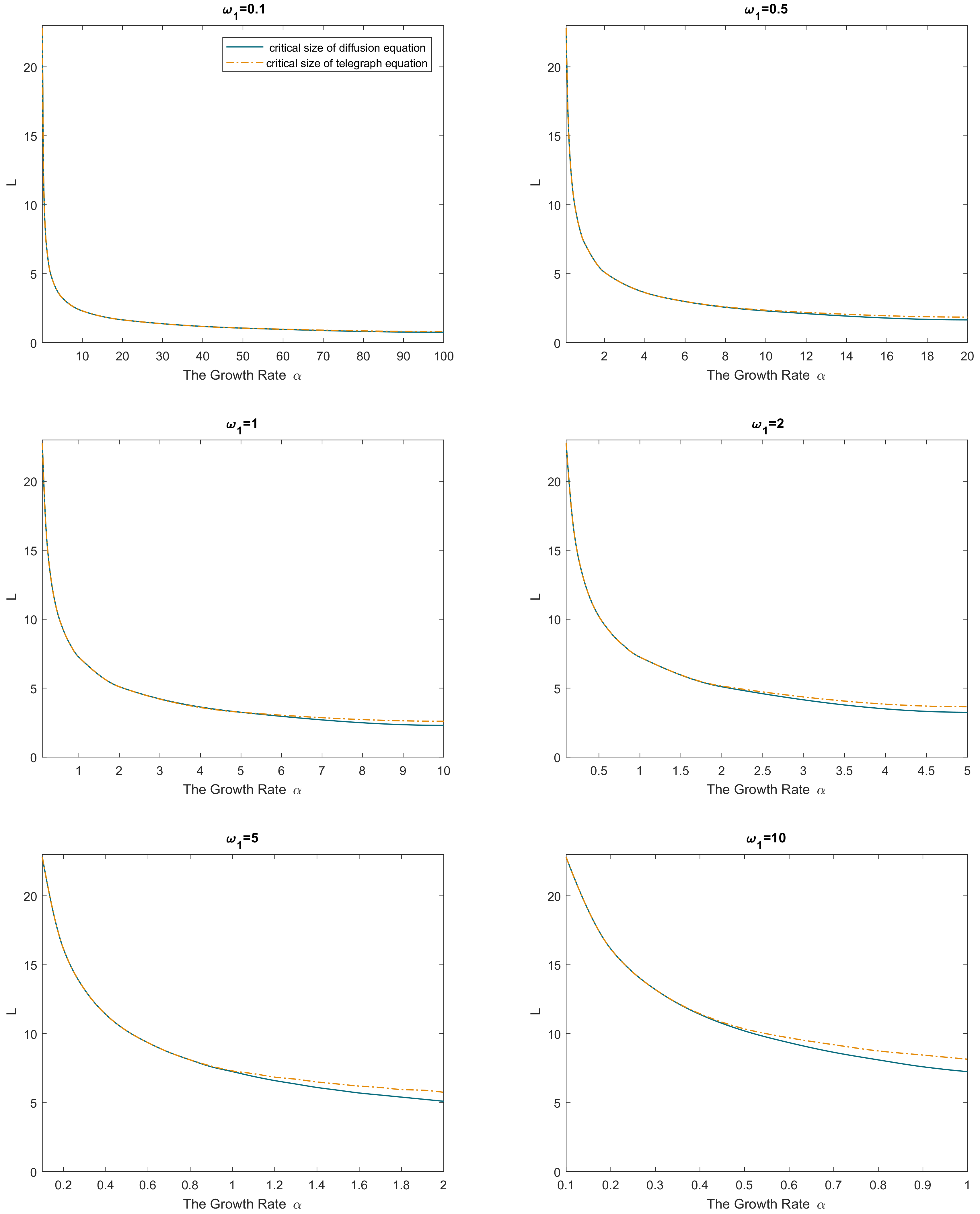
Simulations were performed for different values of varying it in a broad range. For any given set of parameters and , Equation (29) was solved numerically by finite differences (using the implicit method, see Appendix B) in domains of different size L. By distinguishing between the simulation runs resulting in species extinction and those resulting in species persistence, the critical value of the domain size was established. The results are shown in Figure 2. In any panel of the figure, parameter values from below the curve(s) correspond to species extinction in the large-time limit (the domain is not large enough to support sustainable population dynamics), and parameter values from above the curve(s) correspond to species survival. It is readily seen that, for a small value of the critical domain size of the nonlinear reaction–telegraph equation nearly coincides with the critical domain size of the reaction–diffusion equation. This is perhaps not surprising as, intuitively, Equation (29) with may be expected to approximate the diffusion equation. However, the difference between the two models become significant when either is sufficiently large or is sufficiently small. The diffusion equation and the telegraph equation then have a clearly different critical size. Since is a decreasing function of , the largest difference between the models is reached for larger values of .
We therefore observe that, in all cases, the critical domain size of the reaction–telegraph equation appears to be larger than the critical size of the reaction–diffusion equation. In ecological terms, it indicates that survival in small domains is more problematic for species where animals consistently employ the movement pattern with a preferred movement direction (such as the CRW or the telegraph process).
We also consider the population growth with the strong Allee effect:
where is a parameter, . Correspondingly, we observe that now and . Simulation results are shown in Figure 3. Similarly to the above, we observe that the difference between the two models is small if but may become significant if is not small, and the difference tends to be larger for larger values of . As well as above, the critical size of the reaction–telegraph equation is always larger than the critical size of the reaction–diffusion equation.
5. Empirical Model: Telegraph Equation with a Cutoff
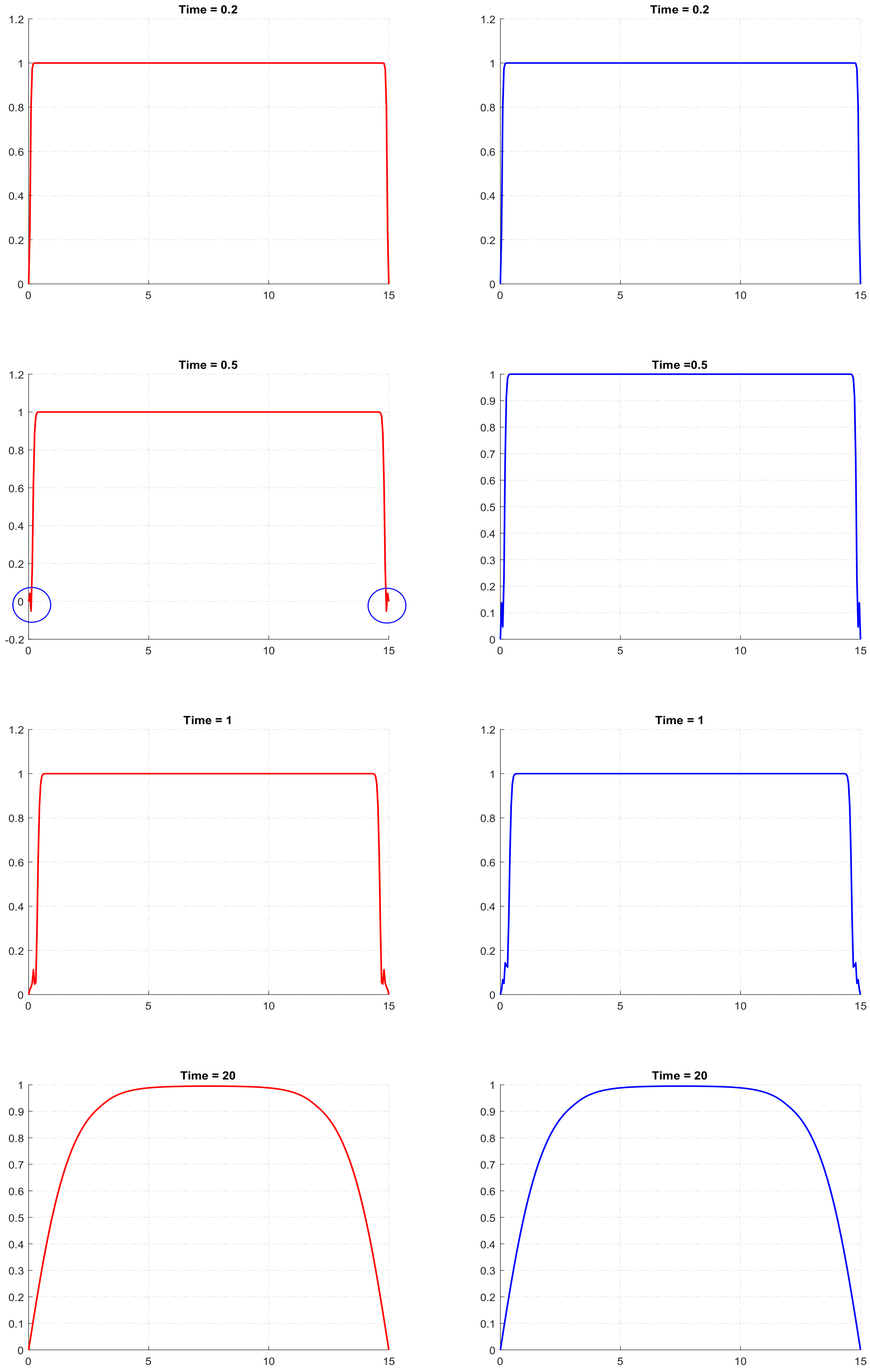
One property of the telegraph equation that can make its application to real-world population dynamics somewhat questionable is that it is not positively defined [29]. It means that, for a certain combination of parameters and for certain initial conditions, its solution can become negative, at least in some areas of the domain and for some intervals of time. In our simulations of the reaction–telegraph equation, we also observed this property. Although it does not seem to be a frequent phenomenon, it may indeed happen for some parameter values. By way of example, the left column in Figure 4 shows the solutions of the reaction–telegraph equation with the logistic growth, where u becomes negative at some locations close to the domain boundary. After being negative for a short time (several time steps in the finite-difference procedure), the solution becomes positive again. We mention here that this negativity of the solution is not a numerical artefact, as essentially the same behaviour is observed for smaller values of the mesh steps.
Questions arise here as to what may be the reason for the non-positivity and whether the model can possibly be amended to avoid this unrealistic behaviour. We mention here that the corresponding microscopic model that considers movement of individual ‘particles’ (e.g., animals) is positively defined [20]. The non-positivity of the solution is therefore an artefact of its mean-field counterpart rather than a genuine property of the movement–reproduction dynamics as such.
One empirical way to keep the solution nonnegative is to introduce a cutoff into the finite-difference method: as soon as , we set . Since we have observed in our simulations that, if the solution becomes negative, it only attains small values, one can expect that the perturbation introduced to the solution by the cutoff is likely to remain small. In order to look into this issue, for the same set of parameter values and initial conditions, we performed simulations with and without cutoff. We obtained that solution of the reaction–telegraph equation was robust to the cutoff procedure and eventually produced almost the same distribution of the population density. The left column in Figure 4 shows the solution without cutoff and the right column shows the solution after a cutoff was implemented at . There is no any visual distinction between the corresponding panels in the left and the right columns of the figure. Similar results are obtained in the case of the strong Allee effect; we do not show them here for sake of brevity.
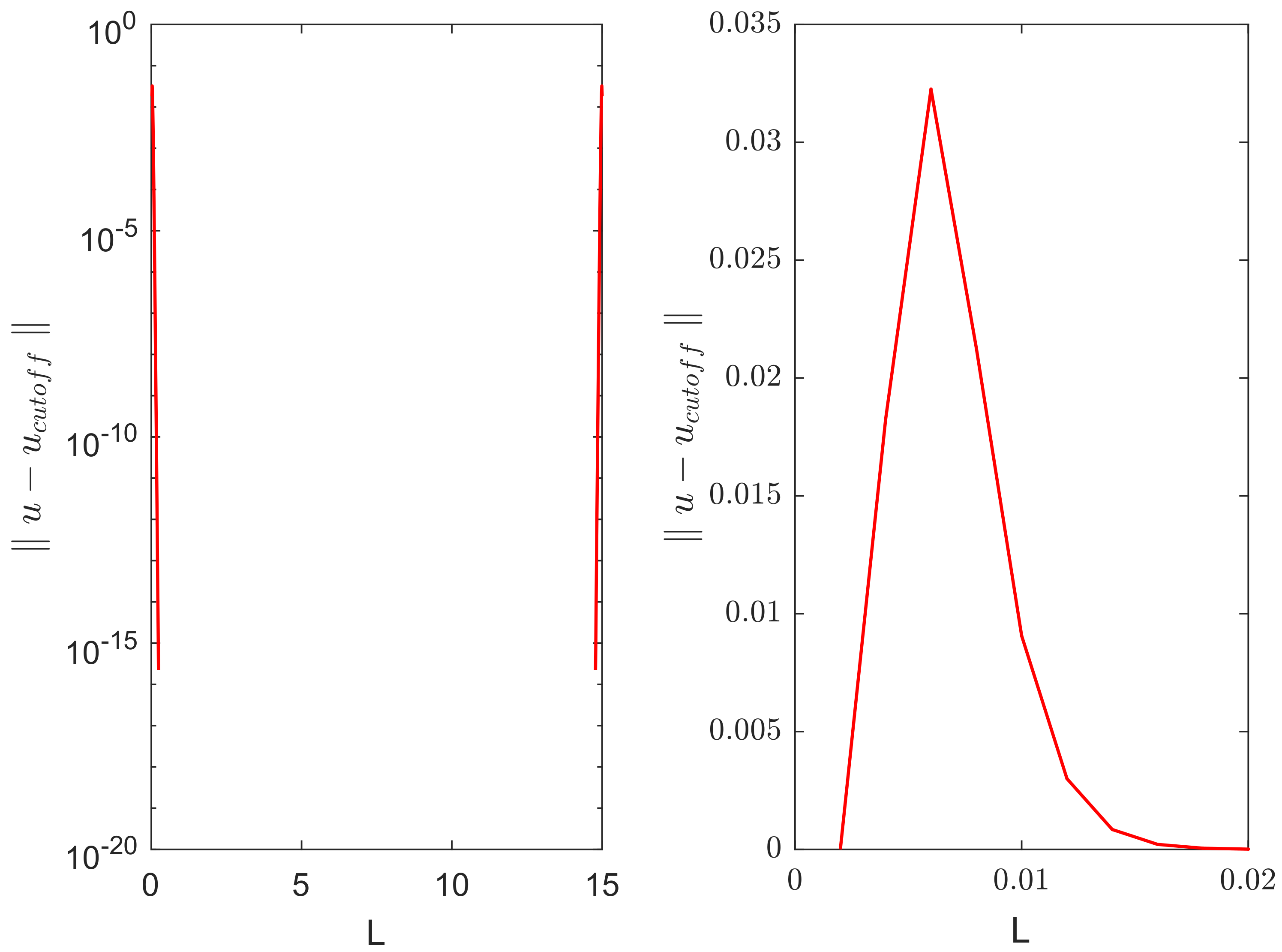
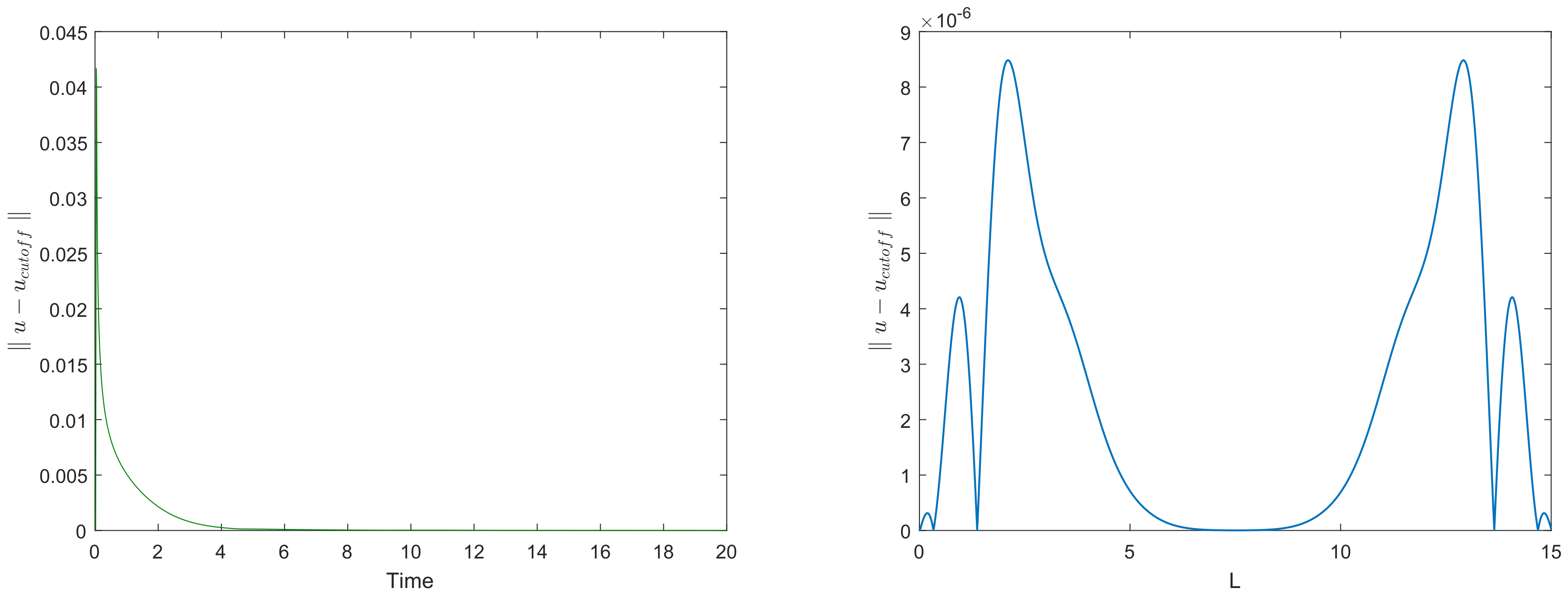
In order to make a more quantitative insight into the evolution of the perturbation introduced by the cutoff, we calculated the ‘error’—the difference between the solutions with and without cutoff—as a function of time and space. Figure 5 shows the distribution of error over the domain at time (i.e., immediately after the cutoff was done), as corresponds to the second row in Figure 4. The error is non-zero only in small areas close to the domain boundaries where the solution became negative. Figure 6 left shows how the maximum error over the domain (i.e., the maximum of functions shown in Figure 5) evolves with time. It is readily seen that the maximum error promptly decays with time, eventually reaching very small values. Figure 6 right shows the distribution of error over space at time , i.e., as corresponds to the bottom row in Figure 4.
6. Discussion and Conclusions
For several decades, the main mathematical framework for modelling animal movement and dispersal was based on the simple isotropic random walk model (SRW) which is unbiased in the sense that, at any moment, the walker can move in any possible direction [13]. This means that the movement direction taken at any given time is independent (uncorrelated) of the movement direction at the preceding moment. The CRW is an extension of the SRW that accounts for the persistence in the walker’s direction of movement [17,19,20,23,30]. Indeed, in most real-world systems, the walker is more likely to move in a direction similar to the previous one. This is known as persistence and it can be combined with a fixed speed of movement in the random walk process, resulting in the telegraph or velocity-jump processes [19,31,32,33]. Our baseline model (1), i.e., the 1D telegraph equation is the mean-field counterpart for the simplest one-dimensional CRW; it includes SRW (the diffusive movement) as the limiting case when the persistence vanishes, i.e., for .
Being thus a model presumably more adequate than the reaction–diffusion equation, questions arise as to what the properties of the reaction–telegraph equation can be in a relevant ecological context and how different they may be from those of the corresponding reaction–diffusion equation. In this paper, we addressed these questions in the context of habitat fragmentation and species survival in small domains. Having considered the critical domain problem for the reaction–telegraph equation, we arrive at the following conclusions:
- In the case of a linear reaction term (i.e., linear population growth), we found that the critical domain size for the reaction–telegraph equation coincides with that of the corresponding reaction–diffusion equation. This seems to be a surprising result as intuitively the more directional animal movement described by the reaction–telegraph equation should result in a larger critical size.
- In the case of a nonlinear growth (either logistic or with a strong Allee effect), we found that the critical size of the reaction–telegraph equation is indeed somewhat larger than that of the corresponding reaction–diffusion equation. Thus, the difference between the two models arise as a result of a subtle interplay between the movement pattern and the nonlinearity of the population growth.
Our study has potentially important implications for ecology and nature conservation, in particular by means of providing better understanding of the effect that biologically meaningful factors (such as the animal movement pattern and the type of the growth rate) may have on the minimum domain size required to prevent extinctions. However, since the reaction–telegraph equation is widely used in various branches of science and engineering, our findings are likely to have broader range of applications. Traditionally, the telegraph equation was used to describe the voltage and current that can be found on electrical transmission line. In particular, the telegraphic equation was studied by Lord Kelvin in relation to the signals that propagate across the transatlantic cable. The telegraph equation has also been used to model various problems in wave propagation and signal analysis more generally [34,35], random walk theory [31], transport in heterogeneous porous media [32] and pulse transmission through a nerve axon [36,37]. It also has applications in other fields, in particular, it has been used to model transport processes in physical, biological, social, and ecological systems [34,38,39,40,41,42,43]. Understanding the problem of critical size in those wide-ranging specific contexts is likely to result in exciting new research.
Acknowledgments
An illuminating discussion of the problem with Paulo F. C. Tilles is acknowledged and appreciated.
Author Contributions
Sergei Petrovskii designed the research. Sergei Petrovskii and Weam Alharbi performed the linear analysis. Weam Alharbi wrote the numerical code and performed simulations. Sergei Petrovskii and Weam Alharbi wrote the manuscript.
Conflicts of Interest
The authors declare no conflicts of interest.
Appendix A. Calculation of the Coefficients in the Fourier Series
Setting in Equation (23) and using the initial condition results in the requirement that
Recognizing that this is just a Fourier Sine Series for the function , the constants must be the coefficients of that Sine Series; therefore:
In order to make use of the second initial condition, we have to differentiate Equation (23) with respect to time:
where is defined by Equation (19). For , from the above equation, we obtain:
This is a Fourier Sine Series for with coefficients as
Therefore,
Appendix B. Numerical Scheme
The implicit scheme at the point for solving Equation (6) is:
where and .
In case growth rate is linear, at each time step, Equation (A6) (where and N is the number of nodes in the spatial grid) is a linear algebraic system and hence is straightforward to solve (e.g., using Thomas algorithm). In case is nonlinear, it can be linearized, e.g., it can be interpolated using the first two term of the Taylor expansion:
where is found analytically. Note that, in Equation (A7), we have made use of the fact that, for a smooth function, its left-hand side derivative coincides with its right-hand side derivative, so that .
The simulation results presented in the main text were obtained for and .
References
- Fahrig, L. Effects of habitat fragmentation on biodiversity. Annu. Rev. Ecol. Evol. Syst. 2003, 34, 487–515. [Google Scholar] [CrossRef]
- Ewers, R.M.; Didham, R.K. Confounding factors in the detection of species responses to habitat fragmentation. Biol. Rev. 2006, 81, 117–142. [Google Scholar] [CrossRef] [PubMed]
- Fischer, J.; Lindenmayer, D.B. Landscape modification and habitat fragmentation: A synthesis. Glob. Ecol. Biogeogr. 2007, 16, 265–280. [Google Scholar] [CrossRef]
- Kirk, R.V.; Lewis, M.A. Edge permeability and population persistence in isolated habitat patches. Nat. Resour. Model. 1999, 12, 37–64. [Google Scholar] [CrossRef]
- Mangel, M. The Theoretical Biologist’s Toolbox: Quantitative Methods for Ecology and Evolutionary Biology; Cambridge University Press: Cambridge, UK, 2006. [Google Scholar]
- Maynard Smith, J. Models in Ecology; Cambridge University Press: Cambridge, UK, 1974. [Google Scholar]
- Kierstead, H.; Slobodkin, L.B. The size of water masses containing plankton blooms. J. Mar. Res. 1953, 12, 141–147. [Google Scholar]
- Lewis, M.A.; Kareiva, P. Allee dynamics and the spread of invading organisms. Theor. Popul. Biol. 1993, 43, 141–158. [Google Scholar] [CrossRef]
- Petrovskii, S.V. Plankton front waves accelerated by marine turbulence. J. Mar. Syst. 1999, 21, 179–188. [Google Scholar] [CrossRef]
- Petrovskii, S.V.; Shigesada, N. Some exact solutions of a generalized Fisher equation related to the problem of biological invasion. Math. Biosci. 2001, 172, 73–94. [Google Scholar] [CrossRef]
- Alharbi, W.G.; Petrovskii, S.V. The impact of fragmented habitat’s size and shape on populations with Allee effect. Math. Modell. Nat. Phenom. 2016, 11, 5–15. [Google Scholar] [CrossRef]
- Fisher, R.A. The wave of advance of advantageous genes. Ann. Eugen. 1937, 7, 355–369. [Google Scholar] [CrossRef]
- Skellam, J.G. Random dispersal in theoretical populations. Biometrika 1951, 38, 196–218. [Google Scholar] [CrossRef] [PubMed]
- Murray, J.D. Mathematical Biology; Springer: Berlin, Germany, 1989. [Google Scholar]
- Malchow, H.; Petrovskii, S.V.; Venturino, E. Spatiotemporal Patterns in Ecology and Epidemiology: Theory, Models, and Simulation; CRC Press: Boca Raton, FL, USA, 2008. [Google Scholar]
- Pyke, G.H. Understanding movements of organisms: It’s time to abandon the Levy foraging hypothesis. Methods Ecol. Evol. 2015, 6, 1–16. [Google Scholar] [CrossRef]
- Kareiva, P.M.; Shigesada, N. Analyzing insect movement as a correlated random walk. Oecologia 1983, 56, 234–238. [Google Scholar] [CrossRef] [PubMed]
- Kac, M. A stochastic model related to the telegrapher equation. Rocky Mt. J. Math. 1974, 4, 497–509. [Google Scholar] [CrossRef]
- Goldstein, S. On diffusion by discontinuous movements and on the telegraph equation. Quart. J. Mech. Appl. Math. 1951, 4, 129–156. [Google Scholar] [CrossRef]
- Holmes, E.E. Are diffusion models too simple? A comparison with telegraph models of invasion. Am. Nat. 1993, 142, 779–795. [Google Scholar] [CrossRef] [PubMed]
- Mainardi, F. Signal velocity for transient waves in linear dissipative media. Wave Motion 1983, 5, 33–41. [Google Scholar] [CrossRef]
- Di Crescenzo, A.; Martinucci, B.; Zacks, S. Telegraph process with elastic boundary at the origin. Methodol. Comput. Appl. Probabil. 2018, 20, 333–352. [Google Scholar] [CrossRef]
- Mendez, V.; Fedotov, S.; Horsthemke, W. Reaction–Transport Systems: Mesoscopic Foundations, Fronts, and Spatial Instabilities; Springer: Berlin, Germany, 2010. [Google Scholar]
- Lewis, M.A.; Petrovskii, S.V.; Potts, J. The Mathematics Behind Biological Invasions. Interdisciplinary Applied Mathematics; Springer: Berlin, Germany, 2016; Volume 44. [Google Scholar]
- Renardy, M.; Rogers, R.C. An Introduction to Partial Differential Equations; Springer: New York, NY, USA, 2006. [Google Scholar]
- Farlow, S.J. Partial Differential Equations for Scientists and Engineers; Dover: New York, NY, USA, 1993. [Google Scholar]
- Miller, W. The technique of variable separation for partial differential equations. In Nonlinear Phenomena; Wolf, K.B., Ed.; Springer: Berlin, Germany, 1983; pp. 184–208. [Google Scholar]
- Tilles, P.F.C.; Petrovskii, S.V. On the consistency of the reaction–telegraph process in finite domains. J. Math. Biol. 2018. in preperation. [Google Scholar]
- Hillen, T. Existence theory for correlated random walks on bounded domains. Canad. Appl. Math. Q. 2010, 18, 1–40. [Google Scholar]
- Turchin, P. Quantitative Analysis of Movement; Sinauer: Sunderland, UK, 1998. [Google Scholar]
- Banasiak, J.; Mika, J.R. Singularly perturbed telegraph equations with applications in the random walk theory. Int. J. Stoch. Anal. 1998, 11, 9–28. [Google Scholar] [CrossRef]
- Berkowitz, B.; Kosakowski, G.; Margolin, G.; Scher, H. Application of continuous time random walk theory to tracer test measurements in fractured and heterogeneous porous media. Groundwater 2001, 39, 593–604. [Google Scholar] [CrossRef]
- Van Gorder, R.A.; Vajravelu, K. Analytical and numerical solutions of the density dependent Nagumo telegraph equation. Nonlinear Anal. 2010, 11, 3923–3929. [Google Scholar] [CrossRef]
- Roussy, G.; Pearce, J.A. Foundations and Industrial Applications of Microwaves and Radio Frequency Fields; John Wiley & Sons: Chichester, UK, 1995. [Google Scholar]
- Jordan, P.M.; Puri, A. Digital signal propagation in dispersive media. J. Appl. Phys. 1999, 85, 1273–1282. [Google Scholar] [CrossRef]
- FitzHugh, R. Impulses and physiological states in theoretical models of nerve membrane. Biophys. J. 1961, 1, 445–466. [Google Scholar] [CrossRef]
- Nagumo, J.; Arimoto, S.; Yoshizawa, S. An active pulse transmission line simulating nerve axon. Proc. IRE 1962, 50, 2061–2070. [Google Scholar] [CrossRef]
- Ahmed, E.; Hassanb, S.Z. On diffusion in some biological and economic systems. Z. Naturforsch. A 2000, 55, 669–672. [Google Scholar] [CrossRef]
- Ahmed, E.; Abdusalam, H.A.; Fahmy, E.S. On telegraph reaction diffusion and coupled map lattice in some biological systems. Int. J. Modern Phys. C 2001, 12, 717–726. [Google Scholar] [CrossRef]
- Giusti, A. Dispersion relations for the time-fractional Cattaneo-Maxwell heat equation. J. Math. Phys. 2018, 59, 013506. [Google Scholar] [CrossRef]
- Harris, P.A.; Garra, R. Nonlinear heat conduction equations with memory: Physical meaning and analytical results. J. Math. Phys. 2017, 58, 063501. [Google Scholar] [CrossRef]
- Mohebbi, A.; Dehghan, M. High order compact solution of the one-space-dimensional linear hyperbolic equation. Numer. Methods Part. Differ. Equ. 2008, 24, 1222–1235. [Google Scholar] [CrossRef]
- Sobolev, S.L. On hyperbolic heat-mass transfer equation. Int. J. Heat Mass Transfer 2018, 122, 629–630. [Google Scholar] [CrossRef]
Figure 1.
Critical domain size of the reaction–telegraph equation obtained numerically at various values of linear growth rate and various values of and as shown by different symbols and different colors. The solid blue curve corresponds to Equation (28). For parameters from below the curve, the population goes to extinction; for parameters from above the curve, the population exhibits unbounded growth.
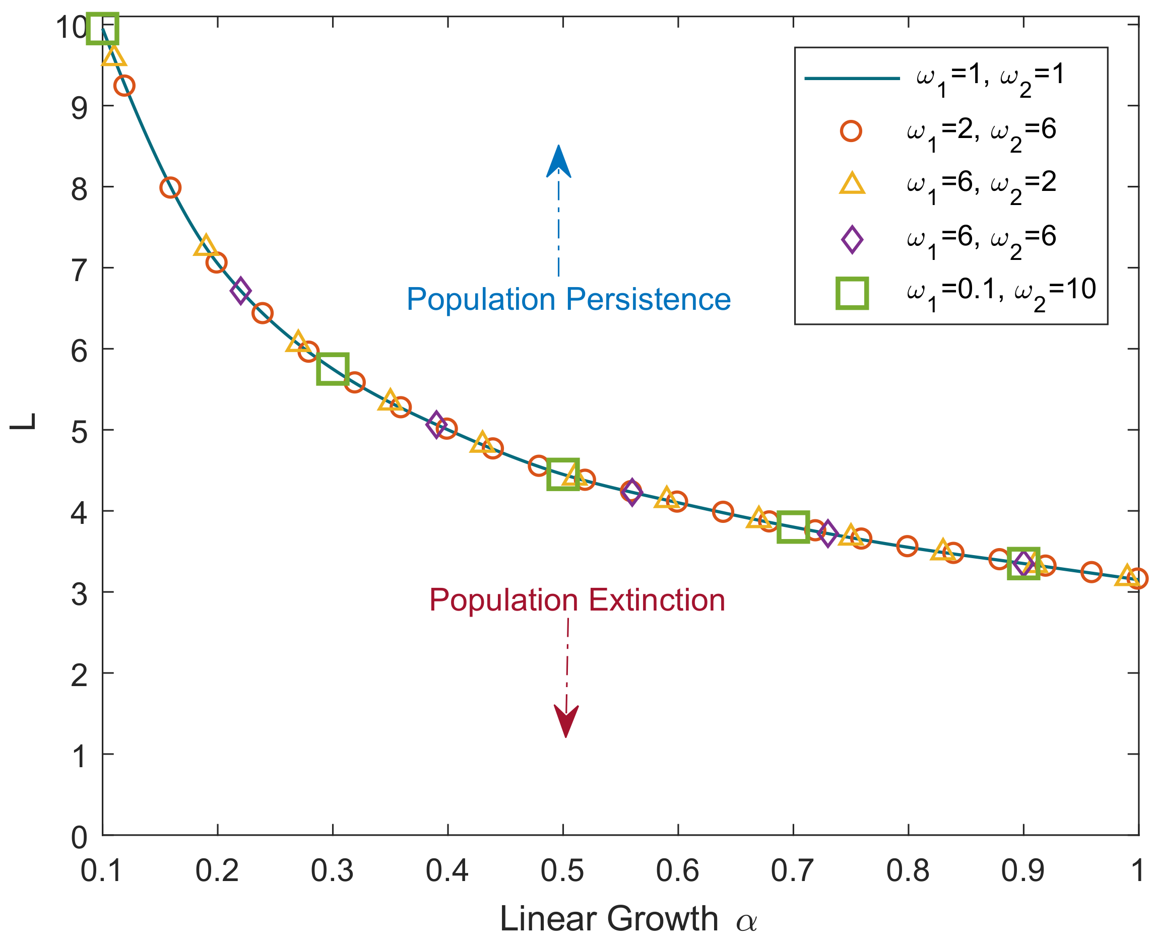
Figure 2.
Dependence of the critical domain size on parameter a α in case the population growth is logistic (see Equation (30)). The dashed black curve shows the results obtained for the reaction–telegraph Equation (29), and the solid red curve shows the results obtained for the corresponding reaction–diffusion equation, i.e., Equation (29) with ω1 = 0. Other parameters are K = 1, D = 1.
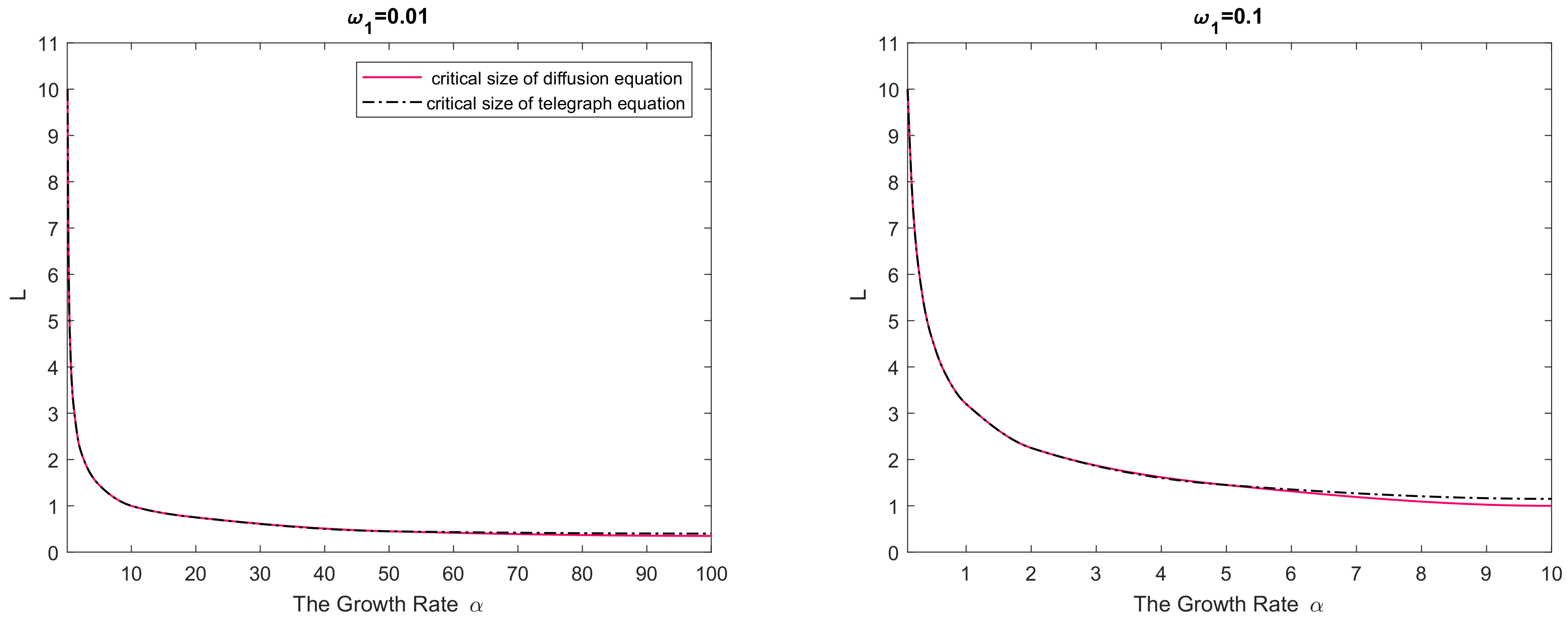
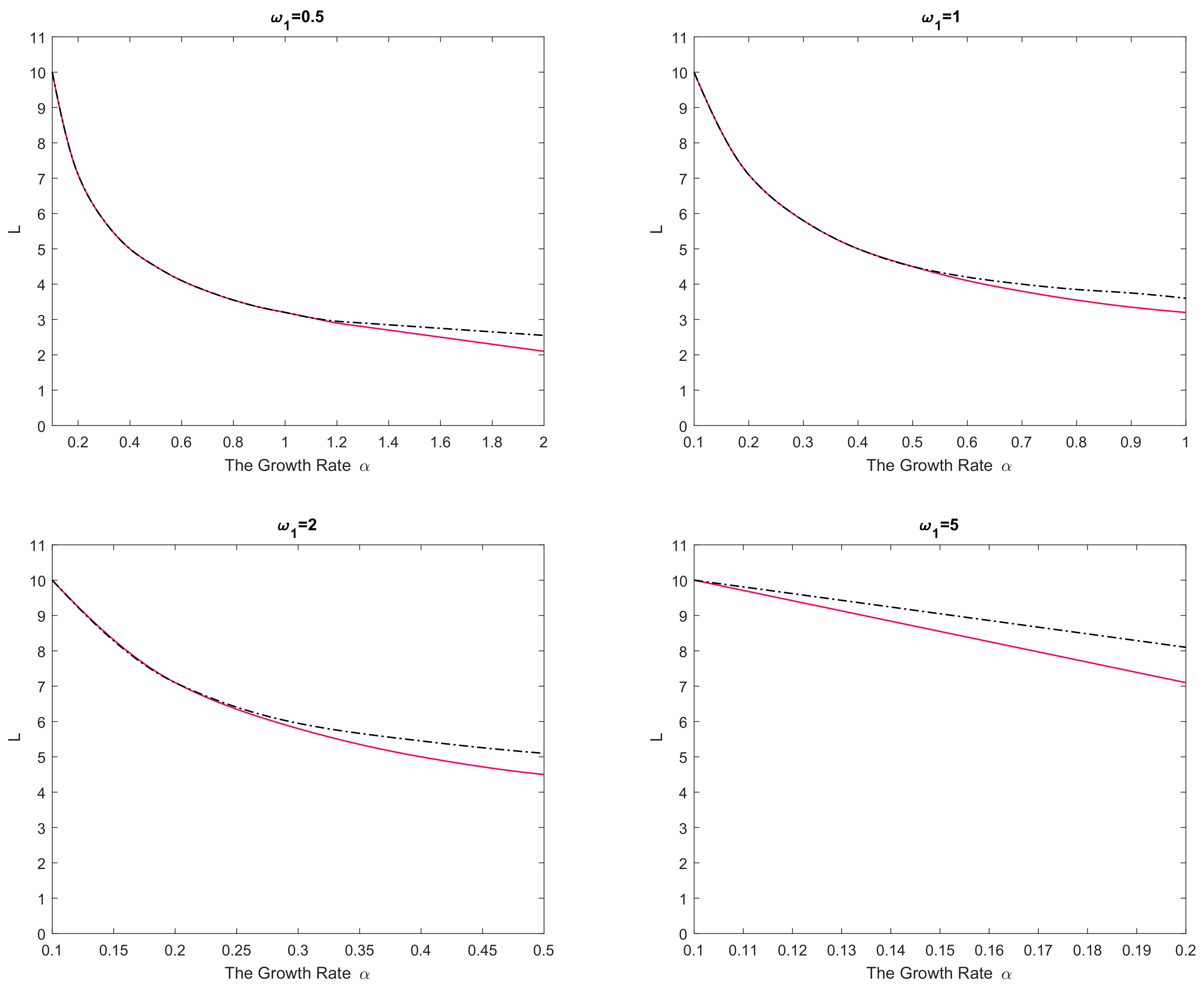
Figure 3.
Dependence of the critical domain size on parameter in case the population growth is subject to the strong Allee effect (see Equation (31)). The dashed orange curve shows the results for the reaction–telegraph Equation (29), and the solid blue curve shows the results obtained for the corresponding reaction–diffusion equation, i.e., Equation (29) with . Other parameters are , , .

Figure 4.
Solution of the reaction–telegraph equation with the logistic growth without cutoff (left, red curves) and with the cutoff of negative values (right, blue curves). Parameters are and . The circles mark the location of the areas where the solution becomes negative.
Figure 4.
Solution of the reaction–telegraph equation with the logistic growth without cutoff (left, red curves) and with the cutoff of negative values (right, blue curves). Parameters are and . The circles mark the location of the areas where the solution becomes negative.

Figure 5.
Distribution of the error over space at , i.e., immediately after the cutoff was implemented. (left) distribution over the whole domain ; (right) a magnified view of the part of the domain close to the left-hand side boundary.
Figure 5.
Distribution of the error over space at , i.e., immediately after the cutoff was implemented. (left) distribution over the whole domain ; (right) a magnified view of the part of the domain close to the left-hand side boundary.

Figure 6.
(left) maximum error as a function of time; (right) distribution of error over the domain at .
Figure 6.
(left) maximum error as a function of time; (right) distribution of error over the domain at .
© 2018 by the authors. Licensee MDPI, Basel, Switzerland. This article is an open access article distributed under the terms and conditions of the Creative Commons Attribution (CC BY) license (http://creativecommons.org/licenses/by/4.0/).
Share and Cite
MDPI and ACS Style
Alharbi, W.; Petrovskii, S. Critical Domain Problem for the Reaction–Telegraph Equation Model of Population Dynamics. Mathematics 2018, 6, 59. https://doi.org/10.3390/math6040059
AMA Style
Alharbi W, Petrovskii S. Critical Domain Problem for the Reaction–Telegraph Equation Model of Population Dynamics. Mathematics. 2018; 6(4):59. https://doi.org/10.3390/math6040059
Chicago/Turabian StyleAlharbi, Weam, and Sergei Petrovskii. 2018. "Critical Domain Problem for the Reaction–Telegraph Equation Model of Population Dynamics" Mathematics 6, no. 4: 59. https://doi.org/10.3390/math6040059
Note that from the first issue of 2016, this journal uses article numbers instead of page numbers. See further details here.