The Modified Beta Gompertz Distribution: Theory and Applications

Abstract

In this paper, we introduce a new continuous probability distribution with five parameters called the modified beta Gompertz distribution. It is derived from the modified beta generator proposed by Nadarajah, Teimouri and Shih (2014) and the Gompertz distribution. By investigating its mathematical and practical aspects, we prove that it is quite flexible and can be used effectively in modeling a wide variety of real phenomena. Among others, we provide useful expansions of crucial functions, quantile function, moments, incomplete moments, moment generating function, entropies and order statistics. We explore the estimation of the model parameters by the obtained maximum likelihood method. We also present a simulation study testing the validity of maximum likelihood estimators. Finally, we illustrate the flexibility of the distribution by the consideration of two real datasets.

1. Introduction

The Gompertz distribution is a continuous probability distribution introduced by Gompertz [1]. The literature about the use of the Gompertz distribution in applied areas is enormous. A nice review can be found in [2], and the references therein. From a mathematical point of view, the cumulative probability density function (cdf) of the Gompertz distribution with parameters $\lambda >0$ and $\alpha >0$ is given by

$$G(x)=1-e^{-\frac{\lambda }{\alpha }(e^{\alpha x}-1)},x>0.$$

The related probability density function (pdf) is given by

$$g(x)=\lambda e^{\alpha x}{e}^{-\frac{\lambda }{\alpha }(e^{\alpha x}-1)},x>0.$$

It can be viewed as a generalization of the exponential distribution (obtained with $\alpha \to 0$) and thus an alternative to the gamma or Weibull distribution. A feature of the Gompertz distribution is that $g(x)$ is unimodal and has positive skewness, whereas the related hazard rate function (hrf) given by $h(x)=g(x)/(1-G(x))$ is increasing. To increase the flexibility of the Gompertz distribution, further extensions have been proposed. A natural one is the generalized Gompertz distribution introduced by El-Gohary et al. [3]. By introducing an exponent parameter $a>0$, the related cdf is given by

$$F(x)={\left(1-e^{-\frac{\lambda }{\alpha }(e^{\alpha x}-1)}\right)}^a,x>0.$$

The related applications show that a plays an important role in term of model flexibility. This idea was then extended by Jafari et al. [4] who used the so-called beta generator introduced by Eugene et al. [5]. The related cdf is given by

$$\begin{array}{cc}\hfill F(x)& =\frac{1}{B(a,b)}{\int }_0^{1-e^{-\frac{\lambda }{\alpha }(e^{\alpha x}-1)}}{t}^{a-1}{(1-t)}^{b-1}dt\hfill \\ & =I_{1-e^{-\frac{\lambda }{\alpha }(e^{\alpha x}-1)}}(a,b),x>0.\hfill \end{array}$$

(1)

where $a,b>0$, $B(a,b)={\int }_0^1{t}^{a-1}{(1-t)}^{b-1}dt$ and $I_x(a,b)=(1/B(a,b)){\int }_0^x{t}^{a-1}{(1-t)}^{b-1}dt$, $x\in [0,1]$. This distribution has been recently extended by Benkhelifa [6] with a five-parameter distribution. It is based on the beta generator and the generalized Gompertz distribution.

Motivated by the emergence of complex data from many applied areas, other extended Gompertz distributions have been proposed in the literature. See for instance, El-Damcese et al. [7] who considered the Odd Generalized Exponential generator introduced by Tahir et al. [8]; Roozegar et al. [9] who used the McDonald generator introduced by Alexander et al. [10]; Refs. [11,12] who applied the transmuted generator introduced by Shaw and Buckley [13]; Chukwu and Ogunde [14] and Lima et al. [15] who used the Kumaraswamy generator; and Benkhelifa [16] and Yaghoobzadeh [17] who considered the Marshall–Olkin generator introduced by Marshall and Olkin [18]; and Shadrokh and Yaghoobzadeh [19] who considered the Beta-G and Geometric generators.

In this paper, we present and study a distribution with five parameters extending the Gompertz distribution. It is based on the modified beta generator developed by Nadarajah et al. [20] (which can also be viewed as a modification of the beta Marshall–Olkin generator developed by Alizadeh et al. [21]). The advantage of this generator is to nicely combine the advantages of the beta generator of Eugene et al. [5] and the Marshall–Olkin generator of Marshall and Olkin [18]. To the best of our knowledge, its application to the Gompertz distribution has never been considered before. We provide a comprehensive description of its general mathematical properties (expansions of the cdf and pdf, quantile function, various kinds of moments, moment generating function, entropies and order statistics). The estimation of the model parameters by maximum likelihood is then discussed. Finally, we explore applications to real datasets that illustrate the usefulness of the proposed model.

The structure of the paper is as follows. Section 2 describes the considered modified beta Gompertz distribution. Some mathematical properties are investigated in Section 3. Section 4 provides the necessary to the estimation of the unknown parameters with the maximum likelihood method. A simulation study is presented, which tests validity of the obtained maximum likelihood estimators. Applications to two real datasets are also given.

2. The Modified Beta Gompertz Distribution

Let $c>0$, $G(x)$ be a cdf and $g(x)$ be a related pdf. The modified beta generator introduced by Nadarajah et al. [20] is characterized by the cdf given by

$$\begin{array}{c}\hfill F(x)=I_{\frac{cG(x)}{1-(1-c)G(x)}}(a,b),\end{array}$$

(2)

By differentiation of $F(x)$, a pdf is given by

$$\begin{array}{c}\hfill f(x)=\frac{c^{a}g(x){\left[G(x)\right]}^{a-1}{\left[1-G(x)\right]}^{b-1}}{B(a,b){\left[1-(1-c)G(x)\right]}^{a+b}},x\in \mathbb{R}.\end{array}$$

(3)

The hrf is given by

$$h(x)=\frac{c^{a}g(x){\left[G(x)\right]}^{a-1}{\left[1-G(x)\right]}^{b-1}}{B(a,b){\left[1-(1-c)G(x)\right]}^{a+b}\left(1-I_{\frac{cG(x)}{1-(1-c)G(x)}}(a,b)\right)},x\in \mathbb{R}.$$

Let us now present our main distribution of interest. Using the cdf $G(x)$ of the Gompertz distribution with parameters $\lambda >0$ and $\alpha >0$ as baseline, the cdf given by Equation (2) becomes

$$\begin{array}{c}\hfill F(x)=I_{\frac{c\left(1-e^{-\frac{\lambda }{\alpha }(e^{\alpha x}-1)}\right)}{1-(1-c)\left(1-e^{-\frac{\lambda }{\alpha }(e^{\alpha x}-1)}\right)}}(a,b),x>0.\end{array}$$

(4)

The related distribution is called the modified beta Gompertz distribution (MBGz distribution), also denoted by MBGz($\lambda ,\alpha ,a,b,c$). The related pdf in Equation (3) is given by

$$\begin{array}{c}\hfill f(x)=\frac{c^a\lambda e^{\alpha x}{e}^{-\frac{\lambda b}{\alpha }(e^{\alpha x}-1)}{\left(1-e^{-\frac{\lambda }{\alpha }(e^{\alpha x}-1)}\right)}^{a-1}}{B(a,b){\left[1-(1-c)\left(1-e^{-\frac{\lambda }{\alpha }(e^{\alpha x}-1)}\right)\right]}^{a+b}},x>0.\end{array}$$

(5)

The hrf is given by

$$\begin{array}{c}h(x)=\hfill \\ \frac{c^a\lambda e^{\alpha x}{e}^{-\frac{\lambda b}{\alpha }(e^{\alpha x}-1)}{\left(1-e^{-\frac{\lambda }{\alpha }(e^{\alpha x}-1)}\right)}^{a-1}}{B(a,b){\left[1-(1-c)\left(1-e^{-\frac{\lambda }{\alpha }(e^{\alpha x}-1)}\right)\right]}^{a+b}\left[1-I_{\frac{c\left(1-e^{-\frac{\lambda }{\alpha }(e^{\alpha x}-1)}\right)}{1-(1-c)\left(1-e^{-\frac{\lambda }{\alpha }(e^{\alpha x}-1)}\right)}}(a,b)\right]},\hfill \\ x>0.\hfill \end{array}$$

(6)

Figure 1 shows the plots for $f(x)$ and $h(x)$ for selected parameter values $\lambda ,\alpha ,a,b,c$. We observe that these functions can take various curvature forms depending on the parameter values, showing the increasing of the flexibility of the former Gompertz distribution.

Figure 1. Some plots of the pdf $f(x)$ (a); and some plots for the hrf $h(x)$ (b).

A strong point of the MBGz distribution is to contain different useful distributions in the literature. The most popular of them are listed below.

• When $c=1/(1-\theta )$ with $\theta \in (0,1)$ ($\theta$ is a proportion parameter), we obtain the beta Gompertz geometric distribution introduced by Shadrokh and Yaghoobzadeh [19], i.e., with cdf

  $$F(x)=I_{\frac{1-e^{-\frac{\lambda }{\alpha }(e^{\alpha x}-1)}}{1-\theta e^{-\frac{\lambda }{\alpha }(e^{\alpha x}-1)}}}(a,b),x>0.$$
  However, this distribution excludes the case $c\in (0,1)$, which is of importance since it contains well-known flexible distributions, as developed below. Moreover, the importance of small values for c can also be determinant in the applications (see Section 4).
• When $c=1$, we get the beta Gompertz distribution with four parameters introduced by Jafari et al. [4], i.e., with cdf

  $$F(x)=I_{1-e^{-\frac{\lambda }{\alpha }(e^{\alpha x}-1)}}(a,b),x>0.$$
• When $c=b=1$, we get the generalized Gompertz distribution studied by El-Gohary et al. [3], i.e., with cdf

  $$F(x)={\left(1-e^{-\frac{\lambda }{\alpha }(e^{\alpha x}-1)}\right)}^a,x>0.$$
• When $a=b=1$ and $c=\frac{1}{\theta }$ with $\theta >1$, we get the a particular case of the Marshall–Olkin extended generalized Gompertz distribution introduced by Benkhelifa [16], i.e., with cdf

  $$F(x)=\frac{1-e^{-\frac{\lambda }{\alpha }(e^{\alpha x}-1)}}{\theta +(1-\theta )\left(1-e^{-\frac{\lambda }{\alpha }(e^{\alpha x}-1)}\right)},x>0.$$
• When $a=b=c=1$, we get the Gompertz distribution introduced by Gompertz [1], i.e., with cdf

  $$F(x)=1-e^{-\frac{\lambda }{\alpha }(e^{\alpha x}-1)},x>0.$$
• When $c=1$ and $\alpha \to 0$, we get beta exponential distribution studied by Nadarajah and Kotz [22], i.e., with cdf

  $$F(x)=I_{1-e^{-\lambda x}}(a,b),x>0.$$
• When $b=c=1$ and $\alpha \to 0$, we get the generalized exponential distribution studied by Gupta and Kundu [23], i.e., with cdf

  $$F(x)={\left(1-e^{-\lambda x}\right)}^a,x>0.$$
• When $a=b=c=1$ and $\alpha \to 0$ we get the exponential distribution, i.e., with cdf

  $$F(x)=1-e^{-\lambda x},x>0.$$

3. Some Mathematical Properties

3.1. On the Shapes of the pdf

The shapes of $f(x)$ given by Equation (5) can be described analytically. As usual, the critical points $x_{\ast }$ of the pdf $f(x)$ satisfies $\frac{\partial }{\partial x}ln(f(x_{\ast }))=0$, with

$$\begin{array}{c}\frac{\partial }{\partial x}ln(f(x))=\alpha -b\lambda e^{\alpha x}+(a-1)\frac{\lambda e^{\alpha x}{e}^{-\frac{\lambda }{\alpha }(e^{\alpha x}-1)}}{1-e^{-\frac{\lambda }{\alpha }(e^{\alpha x}-1)}}+(a+b)(1-c)\frac{\lambda e^{\alpha x}{e}^{-\frac{\lambda }{\alpha }(e^{\alpha x}-1)}}{c+(1-c)e^{-\frac{\lambda }{\alpha }(e^{\alpha x}-1)}}.\hfill \end{array}$$

The point $x_{\ast }$ is a local maximum if $\frac{{\partial }^2}{\partial x^2}ln(f(x_{\ast }))<0$, a local minimum if $\frac{{\partial }^2}{\partial x^2}ln(f(x_{\ast }))>0$ and a point of inflection if $\frac{{\partial }^2}{\partial x^2}ln(f(x_{\ast }))=0$.

Let us now study the asymptotic properties of $f(x)$. We have

$$f(x)\sim \frac{c^a}{B(a,b)}{\lambda }^a{x}^{a-1},x\to 0.$$

Thus, for $a\in (0,1)$, we have ${lim}_{x\to 0}f(x)=+\infty$; for $a=1$, we have ${lim}_{x\to 0}f(x)=bc\lambda$; and, for $a>1$, we have ${lim}_{x\to 0}f(x)=0$. We have

$$f(x)\sim \frac{1}{c^{b}B(a,b)}\lambda e^{\alpha x}{e}^{\frac{\lambda b}{\alpha }}{e}^{-\frac{\lambda b}{\alpha }{e}^{\alpha x}},x\to +\infty .$$

Thus, ${lim}_{x\to +\infty }f(x)=0$ in all cases. Figure 1a illustrates these points for selected parameters.

3.2. On the Shapes of the hrf

Similar to the pdf, the critical points $x_{\ast }$ of the hrf $h(x)$ given by Equation (6) satisfy $\frac{\partial }{\partial x}ln(h(x_{\ast }))=0$, with

$$\begin{array}{c}\frac{\partial }{\partial x}ln(h(x))=\alpha -b\lambda e^{\alpha x}+(a-1)\frac{\lambda e^{\alpha x}{e}^{-\frac{\lambda }{\alpha }(e^{\alpha x}-1)}}{1-e^{-\frac{\lambda }{\alpha }(e^{\alpha x}-1)}}+(a+b)(1-c)\frac{\lambda e^{\alpha x}{e}^{-\frac{\lambda }{\alpha }(e^{\alpha x}-1)}}{c+(1-c)e^{-\frac{\lambda }{\alpha }(e^{\alpha x}-1)}}\hfill \\ +\frac{c^a\lambda e^{\alpha x}{e}^{-\frac{\lambda b}{\alpha }(e^{\alpha x}-1)}{\left(1-e^{-\frac{\lambda }{\alpha }(e^{\alpha x}-1)}\right)}^{a-1}}{B(a,b){\left[1-(1-c)\left(1-e^{-\frac{\lambda }{\alpha }(e^{\alpha x}-1)}\right)\right]}^{a+b}\left[1-I_{\frac{c\left(1-e^{-\frac{\lambda }{\alpha }(e^{\alpha x}-1)}\right)}{1-(1-c)\left(1-e^{-\frac{\lambda }{\alpha }(e^{\alpha x}-1)}\right)}}(a,b)\right]}.\hfill \end{array}$$

Again, the point $x_{\ast }$ is a local maximum if $\frac{{\partial }^2}{\partial x^2}ln(h(x_{\ast }))<0$, a local minimum if $\frac{{\partial }^2}{\partial x^2}ln(h(x_{\ast }))>0$ and a point of inflection if $\frac{{\partial }^2}{\partial x^2}ln(h(x_{\ast }))=0$.

We also have

$$h(x)\sim \frac{c^a}{B(a,b)}{\lambda }^a{x}^{a-1},x\to 0.$$

Thus, for $a\in (0,1)$, we have ${lim}_{x\to 0}h(x)=+\infty$; for $a=1$, we have ${lim}_{x\to 0}h(x)=bc\lambda$; and, for $a>1$, we have ${lim}_{x\to 0}h(x)=0$. We have

$$h(x)\sim b\lambda e^{\alpha x},x\to +\infty .$$

Thus, ${lim}_{x\to +\infty }h(x)=+\infty$ in all cases. Figure 1b illustrates these points for selected parameters.

3.3. Linear Representation

Let us determine useful linear representations for $F(x)$ given by Equation (4) and $f(x)$ given by Equation (5). First, let us suppose that $c\in (0,1)$. It follows from the generalized binomial formula, i.e., ${\displaystyle {(1+z)}^{\gamma }=\sum _{k=0}^{+\infty }\left(\genfrac{}{}{0pt}{}{\gamma }{k}\right)z^k}$ for $\left|z\right|<1$ and $\gamma \in \mathbb{R}$, with ${\displaystyle \left(\genfrac{}{}{0pt}{}{\gamma }{k}\right)=\frac{\gamma (\gamma -1)\dots (\gamma -k+1)}{k!}}$, that

$$\begin{array}{cc}\hfill F(x)& =\frac{1}{B(a,b)}{\int }_0^{\frac{cG(x)}{1-(1-c)G(x)}}{t}^{a-1}{(1-t)}^{b-1}dt\hfill \\ & =\frac{1}{B(a,b)}\sum _{k=0}^{+\infty }\left(\genfrac{}{}{0pt}{}{b-1}{k}\right){(-1)}^k{\int }_0^{\frac{cG(x)}{1-(1-c)G(x)}}{t}^{a+k-1}dt\hfill \\ & =\frac{1}{B(a,b)}\sum _{k=0}^{+\infty }\left(\genfrac{}{}{0pt}{}{b-1}{k}\right)\frac{{(-1)}^k}{a+k}{\left[\frac{cG(x)}{1-(1-c)G(x)}\right]}^{a+k}.\hfill \end{array}$$

On the other hand, using again the generalized binomial formula, we obtain

$$\begin{array}{cc}\hfill {\left[\frac{cG(x)}{1-(1-c)G(x)}\right]}^{a+k}& =c^{a+k}\sum _{\ell =0}^{+\infty }\left(\genfrac{}{}{0pt}{}{-(a+k)}{\ell }\right){(-1)}^{\ell }{(1-c)}^{\ell }{[G(x)]}^{\ell +a+k}.\hfill \end{array}$$

(7)

In a similar manner, we have

$$\begin{array}{c}\hfill {[G(x)]}^{\ell +a+k}={\left[1-e^{-\frac{\lambda }{\alpha }(e^{\alpha x}-1)}\right]}^{\ell +a+k}=\sum _{m=0}^{+\infty }\left(\genfrac{}{}{0pt}{}{\ell +a+k}{m}\right){(-1)}^m(1-H_m(x)),\end{array}$$

where $H_m(x)=1-e^{-\frac{m\lambda }{\alpha }(e^{\alpha x}-1)}$ is the cdf of a Gompertz distribution with parameters $m\lambda$ and $\alpha$. Combining these equalities, we obtain the following series expansion:

$$\begin{array}{c}\hfill F(x)=\sum _{m=0}^{+\infty }{v}_m(1-H_m(x)),\end{array}$$

(8)

where

$$v_m=\frac{{(-1)}^m}{B(a,b)}\sum _{k=0}^{+\infty }\sum _{\ell =0}^{+\infty }\left(\genfrac{}{}{0pt}{}{\ell +a+k}{m}\right)\left(\genfrac{}{}{0pt}{}{-(a+k)}{\ell }\right)\left(\genfrac{}{}{0pt}{}{b-1}{k}\right)c^{a+k}{(-1)}^{k+\ell }{(1-c)}^{\ell }\frac{1}{a+k}.$$

By derivation of $F(x)$, $f(x)$ can be expressed as

$$\begin{array}{c}\hfill f(x)=\sum _{m=0}^{+\infty }{w}_m{h}_m(x),\end{array}$$

(9)

where $w_m=-v_m$ and $h_m(x)$ is the pdf of a Gompertz distribution with parameters $m\lambda$ and $\alpha$.

For the case $c>1$, we must do some transformation for Equation (7) to apply the generalized binomial formula. We can write

$$\begin{array}{cc}\hfill {\left[\frac{cG(x)}{1-(1-c)G(x)}\right]}^{a+k}& ={\left[\frac{G(x)}{1-(1-\frac{1}{c})(1-G(x))}\right]}^{a+k}\hfill \\ & ={[G(x)]}^{a+k}\sum _{\ell =0}^{+\infty }\left(\genfrac{}{}{0pt}{}{-(a+k)}{\ell }\right){(-1)}^{\ell }{(c-1)}^{\ell }{c}^{-\ell }{[1-G(x)]}^{\ell }\hfill \\ & =\sum _{\ell =0}^{+\infty }\sum _{q=0}^{\ell }\left(\genfrac{}{}{0pt}{}{-(a+k)}{\ell }\right)\left(\genfrac{}{}{0pt}{}{\ell }{q}\right){(-1)}^{\ell +q}{(c-1)}^{\ell }{c}^{-\ell }{[G(x)]}^{q+a+k}.\hfill \end{array}$$

On the other hand, we have

$$\begin{array}{cc}\hfill {[G(x)]}^{q+a+k}& =\sum _{m=0}^{+\infty }\left(\genfrac{}{}{0pt}{}{q+a+k}{m}\right){(-1)}^m(1-H_m(x)).\hfill \end{array}$$

Therefore, we can write $F(x)$ as Equation (8) with

$$\begin{array}{c}{v}_m^{\ast }=\hfill \\ \frac{{(-1)}^m}{B(a,b)}\sum _{k=0}^{+\infty }\sum _{\ell =0}^{+\infty }\sum _{q=0}^{\ell }\left(\genfrac{}{}{0pt}{}{-(a+k)}{\ell }\right)\left(\genfrac{}{}{0pt}{}{\ell }{q}\right)\left(\genfrac{}{}{0pt}{}{q+a+k}{m}\right)\left(\genfrac{}{}{0pt}{}{b-1}{k}\right){(-1)}^{\ell +q+k}{(c-1)}^{\ell }{c}^{-\ell }\frac{1}{a+k},\hfill \end{array}$$

and $f(x)$ as Equation (9) with $w_m=-v_m^{\ast }$ (and still $h_m(x)$ is the pdf of a Gompertz distribution with parameters $m\lambda$ and $\alpha$). For the sake of simplicity, we refer to the form in Equation (9) far all series representation of $f(x)$, whether $c\in (0,1)$ or $c>1$.

Hereafter, we denote by X a random variable having the cdf $F(x)$ given by Equation (4) (and the pdf $f(x)$ given by Equation (5)) and by $Y_m$ a random variable following the Gompertz distribution with parameters $m\lambda$ and $\alpha$, i.e., having the cdf $H_m(x)$ (and the pdf $h_m(x)$).

3.4. Quantile Function

The quantile function of X is given by

$$Q(u)=\frac{1}{\alpha }ln\left(1-\frac{\alpha }{\lambda }ln\left(1-\frac{I_u^{-1}(a,b)}{c+(1-c)I_u^{-1}(a,b)}\right)\right),u\in (0,1),$$

where $I_u^{-1}(a,b)$ denotes the inverse of $I_u(a,b)$. It satisfies $F(Q(u))=Q(F(u))=u$. Using [20], one can show that

$$Q(u)\sim \frac{1}{\lambda c}{a}^{\frac{1}{a}}B{(a,b)}^{\frac{1}{a}}{u}^{\frac{1}{a}},u\to 0.$$

From $Q(u)$, we can simulate the MBGz distribution. Indeed, let U be a random variable following the uniform distribution over $(0,1)$. Then, the random variable $X=Q(U)$ follows the MBGz distribution.

The median of X is given by $M=Q(1/2)$. We can also use $Q(u)$ to define skewness measures. Let us just introduce the Bowley skewness based on quartiles and the Moors kurtosis respectively defined by

$$B=\frac{Q(3/4)+Q(1/4)-2Q(1/2)}{Q(3/4)-Q(1/4)},M_o=\frac{Q(7/8)-Q(5/8)+Q(3/8)-Q(1/8)}{Q(6/8)-Q(2/8)}.$$

Contrary to ${\gamma }_1$ and ${\gamma }_2$, these quantities have the advantage to be always defined. We refer to [24,25].

3.5. Moments

Let r be a positive integer. The rth ordinary moment of X is defined by ${\mu }_r^{\prime }=\mathbb{E}\left(X^r\right)={\int }_{-\infty }^{+\infty }{x}^{r}f(x)dx$. Using the linear representation given by Equation (9), we can express ${\mu }_r^{\prime }$ as

$${\mu }_r^{\prime }=\sum _{m=0}^{+\infty }{w}_m{\int }_{-\infty }^{+\infty }{x}^r{h}_m(x)dx=\sum _{m=0}^{+\infty }{w}_m\mathbb{E}(Y_m^r).$$

By doing the change of variables $u=e^{\alpha x}$, we obtain

$$\mathbb{E}(Y_m^r)=\frac{m\lambda }{{\alpha }^{r+1}}{e}^{\frac{m\lambda }{\alpha }}{\int }_1^{+\infty }{(lnu)}^r{e}^{-\frac{m\lambda }{\alpha }u}du.$$

This integral has connections with the so-called generalized integro-exponential function. Further developments can be found in [26,27]. Therefore, we have

$${\mu }_r^{\prime }=\sum _{m=0}^{+\infty }{w}_m\frac{m\lambda }{{\alpha }^{r+1}}{e}^{\frac{m\lambda }{\alpha }}{\int }_1^{+\infty }{(lnu)}^r{e}^{-\frac{m\lambda }{\alpha }u}du.$$

Obviously, the mean of X is given by $\mathbb{E}(X)={\mu }_1^{\prime }$ and the variance of X is given by $\mathbb{V}(X)={\mu }_2^{\prime }-{({\mu }_1^{\prime })}^2$.

3.6. Skewness

The rth central moment of X is given by ${\mu }_r=\mathbb{E}\left[{(X-{\mu }_1^{\prime })}^r\right]$. It follows from the binomial formula that

$${\mu }_r=\sum _{k=0}^r\left(\genfrac{}{}{0pt}{}{r}{k}\right){(-1)}^k{({\mu }_1^{\prime })}^k{\mu }_{r-k}^{\prime }.$$

On the other side, the rth cumulants of X can be obtained via the equation:

$${\kappa }_r={\mu }_r^{\prime }-\sum _{k=1}^{r-1}\left(\genfrac{}{}{0pt}{}{r-1}{k-1}\right){\kappa }_k{\mu }_{r-k}^{\prime },$$

with ${\kappa }_1={\mu }_1^{\prime }$. The skewness of X is given by ${\gamma }_1={\kappa }_3/{\kappa }_2^{3/2}$ and the kurtosis of X is given by ${\gamma }_2={\kappa }_4/{\kappa }_2^2$. One can also introduce the MacGillivray skewness given by

$$\rho (u)=\frac{Q(1-u)+Q(u)-2Q(1/2)}{Q(1-u)-Q(u)},u\in (0,1).$$

It illustrates the effects of the parameters a, b, $\alpha$ and $\lambda$ on the skewness. Further details can be found in [28].

3.7. Moment Generating Function

The moment generating function of X is given by $M_X(t)=\mathbb{E}\left(e^{tX}\right)={\int }_{-\infty }^{+\infty }{e}^{tx}f(x)dx$. Using Equation (9), we have

$$M_X(t)=\sum _{m=0}^{+\infty }{w}_m{\int }_{-\infty }^{+\infty }{e}^{tx}{h}_m(x)dx=\sum _{m=0}^{+\infty }{w}_m{M}_{Y_m}(t),$$

where $M_{Y_m}(t)=\mathbb{E}(e^{t{Y}_m})$, the moment generating function of $Y_m$. Doing successively the change of variables $u=e^{\alpha x}$ and the change of variable $v=\frac{m\lambda }{\alpha }u$, we obtain

$$\begin{array}{cc}\hfill M_{Y_m}(t)& =\frac{m\lambda }{\alpha }{e}^{\frac{m\lambda }{\alpha }}{\int }_1^{+\infty }{u}^{\frac{t}{\alpha }}{e}^{-\frac{m\lambda }{\alpha }u}du=e^{\frac{m\lambda }{\alpha }}{\left(\frac{\alpha }{m\lambda }\right)}^{\frac{t}{\alpha }}{\int }_{\frac{m\lambda }{\alpha }}^{+\infty }{v}^{\frac{t}{\alpha }}{e}^{-v}dv\hfill \\ & =e^{\frac{m\lambda }{\alpha }}{\left(\frac{\alpha }{m\lambda }\right)}^{\frac{t}{\alpha }}\mathsf{\Gamma }\left(\frac{t}{\alpha }+1,\frac{m\lambda }{\alpha }\right),\hfill \end{array}$$

where $\mathsf{\Gamma }(d,x)$ denotes the complementary incomplete gamma function defined by $\mathsf{\Gamma }(d,x)={\int }_x^{+\infty }{t}^{d-1}{e}^{-t}dt$. Therefore, we can write

$$M_X(t)=\sum _{m=0}^{+\infty }{w}_m{e}^{\frac{m\lambda }{\alpha }}{\left(\frac{\alpha }{m\lambda }\right)}^{\frac{t}{\alpha }}\mathsf{\Gamma }\left(\frac{t}{\alpha }+1,\frac{m\lambda }{\alpha }\right).$$

Alternatively, using the moments of X, one can write

$$M_X(t)=\sum _{r=0}^{+\infty }\frac{t^r}{r!}{\mu }_r^{\prime }=\sum _{r=0}^{+\infty }\sum _{m=0}^{+\infty }\frac{t^r}{r!}{w}_m\frac{m\lambda }{{\alpha }^{r+1}}{e}^{\frac{m\lambda }{\alpha }}{\int }_1^{+\infty }{(lnu)}^r{e}^{-\frac{m\lambda }{\alpha }u}du.$$

3.8. Incomplete Moments and Mean Deviations

The rth incomplete moment of X is defined by $m_r(t)=\mathbb{E}\left(X^r{1}_{\{X\le t\}}\right)={\int }_{-\infty }^t{x}^{r}f(x)dx$. Using Equation (9), we can express $m_r(t)$ as

$$m_r(t)=\sum _{m=0}^{+\infty }{w}_m{\int }_{-\infty }^t{x}^r{h}_m(x)dx.$$

Doing successively the change of variables $u=e^{\alpha x}$, we obtain

$$\begin{array}{c}\hfill {\int }_{-\infty }^t{x}^r{h}_m(x)dx=\frac{m\lambda }{{\alpha }^{r+1}}{e}^{\frac{m\lambda }{\alpha }}{\int }_1^{e^{\alpha t}}{(lnu)}^r{e}^{-\frac{m\lambda }{\alpha }u}du.\end{array}$$

The mean deviation of X about the mean is given by

$${\delta }_1=\mathbb{E}(|X-{\mu }_1^{\prime }|)=2{\mu }_1^{\prime }F({\mu }_1^{\prime })-2m_1({\mu }_1^{\prime }),$$

where $m_1(t)$ denote the first incomplete moment. The mean deviation of X about the median $M=Q(1/2)$ is given by

$${\delta }_2=\mathbb{E}(|X-M|)={\mu }_1^{\prime }-2m_1(M).$$

3.9. Entropies

Let us now investigate different kinds of entropies. For the sake of simplicity in exposition, we suppose that $c\in (0,1)$ (the case $c>1$ can be considered in a similar way). The Rényi entropy of X is defined by

$${\mathcal{I}}_{\gamma }(X)=\frac{1}{1-\gamma }ln\left[{\int }_{-\infty }^{+\infty }{\left[f(x)\right]}^{\gamma }dx\right],$$

with $\gamma >0$ and $\gamma \ne 1$. It follows from (3) that

$${\left[f(x)\right]}^{\gamma }=\frac{c^{a\gamma }{[g(x)]}^{\gamma }{\left[G(x)\right]}^{\gamma (a-1)}{\left[1-G(x)\right]}^{\gamma (b-1)}}{B{(a,b)}^{\gamma }{\left[1-(1-c)G(x)\right]}^{\gamma (a+b)}}.$$

The generalized binomial formula implies that

$$\begin{array}{cc}\hfill \frac{{\left[G(x)\right]}^{\gamma (a-1)}}{{\left[1-(1-c)G(x)\right]}^{\gamma (a+b)}}& =\sum _{k=0}^{+\infty }\left(\genfrac{}{}{0pt}{}{-\gamma (a+b)}{k}\right){(-1)}^k{(1-c)}^k{[G(x)]}^{k+\gamma (a-1)}.\hfill \end{array}$$

Similarly, we have

$$\begin{array}{c}\hfill {[G(x)]}^{k+\gamma (a-1)}=\sum _{\ell =0}^{+\infty }\left(\genfrac{}{}{0pt}{}{k+\gamma (a-1)}{\ell }\right){(-1)}^{\ell }{[1-G(x)]}^{\ell }.\end{array}$$

Therefore,

$$\begin{array}{c}{\left[f(x)\right]}^{\gamma }=\hfill \\ \frac{c^{a\gamma }}{B{(a,b)}^{\gamma }}\sum _{k=0}^{+\infty }\sum _{\ell =0}^{+\infty }\left(\genfrac{}{}{0pt}{}{-\gamma (a+b)}{k}\right)\left(\genfrac{}{}{0pt}{}{k+\gamma (a-1)}{\ell }\right){(-1)}^{k+\ell }{(1-c)}^k{[1-G(x)]}^{\ell +\gamma (b-1)}{[g(x)]}^{\gamma }.\hfill \end{array}$$

By doing the change of variable $u=e^{\alpha x}$ and the change of variable $v=(\ell +\gamma b)\frac{\lambda }{\alpha }u$, we get

$$\begin{array}{cc}\hfill {\int }_{-\infty }^{+\infty }{[1-G(x)]}^{\ell +\gamma (b-1)}{[g(x)]}^{\gamma }dx& ={\int }_0^{+\infty }{e}^{-(\ell +\gamma b)\frac{\lambda }{\alpha }(e^{\alpha x}-1)}{\lambda }^{\gamma }{e}^{\alpha \gamma x}dx\hfill \\ & ={\lambda }^{\gamma }\frac{1}{\alpha }{e}^{(\ell +\gamma b)\frac{\lambda }{\alpha }}{\int }_1^{+\infty }{u}^{\gamma -1}{e}^{-(\ell +\gamma b)\frac{\lambda }{\alpha }u}du\hfill \\ & =\frac{{\alpha }^{\gamma -1}}{{(\ell +\gamma b)}^{\gamma }}{e}^{(\ell +\gamma b)\frac{\lambda }{\alpha }}{\int }_{(\ell +\gamma b)\frac{\lambda }{\alpha }}^{+\infty }{v}^{\gamma -1}{e}^{-v}dv\hfill \\ & =\frac{{\alpha }^{\gamma -1}}{{(\ell +\gamma b)}^{\gamma }}{e}^{(\ell +\gamma b)\frac{\lambda }{\alpha }}\mathsf{\Gamma }\left(\gamma ,(\ell +\gamma b)\frac{\lambda }{\alpha }\right).\hfill \end{array}$$

By putting the above equalities together, we have

$$\begin{array}{c}{\mathcal{I}}_{\gamma }(X)=\hfill \\ \frac{1}{1-\gamma }[\alpha \gamma ln(c)-\gamma ln(B(a,b))+(\gamma -1)ln(\alpha )+\frac{\gamma b\lambda }{\alpha }\hfill \\ +ln\left[\sum _{k=0}^{+\infty }\sum _{\ell =0}^{+\infty }\left(\genfrac{}{}{0pt}{}{-\gamma (a+b)}{k}\right)\left(\genfrac{}{}{0pt}{}{k+\gamma (a-1)}{\ell }\right){(-1)}^{k+\ell }{(1-c)}^k\frac{e^{\ell \frac{\lambda }{\alpha }}}{{(\ell +\gamma b)}^{\gamma }}\mathsf{\Gamma }\left(\gamma ,(\ell +\gamma b)\frac{\lambda }{\alpha }\right)\right]].\hfill \end{array}$$

The Shannon entropy of X is defined by $S(X)=\mathbb{E}(-ln[f(X)])$. It can be obtained by the formula $S(X)={lim}_{\gamma \to 1^{+}}{\mathcal{I}}_{\gamma }(X)$.

The $\gamma$-entropy is defined by

$$H_{\gamma }(X)=\frac{1}{\gamma -1}ln\left[1-{\int }_{-\infty }^{+\infty }{\left[f(x)\right]}^{\gamma }dx\right].$$

Using the expansion above, we obtain

$$\begin{array}{c}{H}_{\gamma }(X)=\frac{1}{\gamma -1}ln[1-\frac{c^{a\gamma }{\alpha }^{\gamma -1}{e}^{\gamma b\frac{\lambda }{\alpha }}}{B{(a,b)}^{\gamma }}\times \hfill \\ \sum _{k=0}^{+\infty }\sum _{\ell =0}^{+\infty }\left(\genfrac{}{}{0pt}{}{-\gamma (a+b)}{k}\right)\left(\genfrac{}{}{0pt}{}{k+\gamma (a-1)}{\ell }\right){(-1)}^{k+\ell }{(1-c)}^k\frac{e^{\ell \frac{\lambda }{\alpha }}}{{(\ell +\gamma b)}^{\gamma }}\mathsf{\Gamma }\left(\gamma ,(\ell +\gamma b)\frac{\lambda }{\alpha }\right)].\hfill \end{array}$$

3.10. Order Statistics

Let $X_1,\dots ,X_n$ be the random sample from X and $X_{i:n}$ be the ith order statistic. Then, the pdf of $X_{i:n}$ is given by

$$\begin{array}{cc}\hfill f_{i:n}(x)& =\frac{n!}{(i-1)!(n-i)!}f(x){[F(x)]}^{i-1}{\left[1-F(x)\right]}^{n-i}\hfill \\ & =\frac{n!}{(i-1)!(n-i)!}\sum _{j=0}^{n-i}\left(\genfrac{}{}{0pt}{}{n-i}{j}\right){(-1)}^{j}f(x){[F(x)]}^{j+i-1}.\hfill \end{array}$$

It follows from Equations (8) and (9) that

$$f_{i:n}(x)=\frac{n!}{(i-1)!(n-i)!}\sum _{j=0}^{n-i}\left(\genfrac{}{}{0pt}{}{n-i}{j}\right){(-1)}^j\sum _{m=0}^{+\infty }{w}_m{h}_m(x){\left[\sum _{k=0}^{+\infty }{v}_k(1-H_k(x))\right]}^{j+i-1}.$$

Using a result from [29], power series raised to a positive power as follows

$$\begin{array}{c}\hfill {\left(\sum _{k=0}^{+\infty }{a}_k{x}^k\right)}^n=\sum _{k=0}^{+\infty }{d}_{n,k}{x}^k,\end{array}$$

where the coefficients ${(d_{n,k})}_{k\in \mathbb{N}}$ are determined from the recurrence equation: $d_{n,0}=a_0^n$ and, for any $m\ge 1$, $d_{n,m}=(1/(m{a}_0)){\displaystyle \sum _{k=1}^m(k(n+1)-m)a_k{d}_{n,m-k}}$. Therefore, noticing that $1-H_k(x)={\left(e^{-\frac{\lambda }{\alpha }(e^{\alpha x}-1)}\right)}^k$, we have

$${\left[\sum _{k=0}^{+\infty }{v}_k(1-H_k(x))\right]}^{j+i-1}=\sum _{k=0}^{+\infty }{d}_{j+i-1,k}(1-H_k(x)),$$

where $d_{j+i-1,0}=v_0^{j+i-1}$ and, for any $m\ge 1$, $d_{j+i-1,m}=\frac{1}{m{v}_0}{\displaystyle \sum _{k=1}^m(k(j+i)-m)v_k{d}_{j+i-1,m-k}}$. By combining the equalities above, we obtain

$$f_{i:n}(x)=\frac{n!}{(i-1)!(n-i)!}\sum _{j=0}^{n-i}\left(\genfrac{}{}{0pt}{}{n-i}{j}\right){(-1)}^j\sum _{m=0}^{+\infty }\sum _{k=0}^{+\infty }{w}_m{d}_{j+i-1,k}{h}_m(x)(1-H_k(x)).$$

Finally, one can observe that $h_m(x)(1-H_k(x))=m\lambda e^{\alpha x}{e}^{-\frac{(m+k)\lambda }{\alpha }(e^{\alpha x}-1)}=\frac{m}{m+k}{u}_{m+k}(x)$, where $u_{m+k}(x)$ denotes the pdf of the Gompertz distribution with parameters $(m+k)\lambda$ and $\alpha$. Thus, the pdf of ith order statistic of the MBGz distribution can be expressed as a linear combination of Gompertz pdfs, i.e.,

$$f_{i:n}(x)=\frac{n!}{(i-1)!(n-i)!}\sum _{j=0}^{n-i}\left(\genfrac{}{}{0pt}{}{n-i}{j}\right){(-1)}^j\sum _{m=0}^{+\infty }\sum _{k=0}^{+\infty }{w}_m{d}_{j+i-1,k}\frac{m}{m+k}{u}_{m+k}(x).$$

Let r be a positive integer. Then, the rth ordinary moment of $X_{i:n}$ can be expressed as

$$\begin{array}{c}\mathbb{E}(X_{i:n}^r)={\int }_{-\infty }^{+\infty }{x}^r{f}_{i:n}(x)dx\hfill \\ =\frac{n!}{(i-1)!(n-i)!}\sum _{j=0}^{n-i}\left(\genfrac{}{}{0pt}{}{n-i}{j}\right){(-1)}^j\sum _{m=0}^{+\infty }\sum _{k=0}^{+\infty }{w}_m{d}_{j+i-1,k}\frac{m\lambda }{{\alpha }^{r+1}}{e}^{\frac{(m+k)\lambda }{\alpha }}{\int }_1^{+\infty }{(lnu)}^r{e}^{-\frac{(m+k)\lambda }{\alpha }u}du.\hfill \end{array}$$

4. Statistical Inference

4.1. Maximum Likelihood Estimation

We now investigate the estimation of the parameters of the MBGz distribution. Let $x_1,\dots ,x_n$ be n observed values from the MBGz distribution and $\xi =(\lambda ,\alpha ,a,b,c)$ be the vector of unknown parameters. The log likelihood function is given by

$$\begin{array}{cc}\hfill \ell (\xi )& =anln(c)+nln(\lambda )+\alpha \sum _{i=1}^n{x}_i-\frac{\lambda b}{\alpha }\sum _{i=1}^n(e^{\alpha x_i}-1)+(a-1)\sum _{i=1}^{n}ln\left(1-e^{-\frac{\lambda }{\alpha }(e^{\alpha x_i}-1)}\right)\hfill \\ & -nln(B(a,b))-(a+b)\sum _{i=1}^{n}ln\left[1-(1-c)\left(1-e^{-\frac{\lambda }{\alpha }(e^{\alpha x_i}-1)}\right)\right].\hfill \end{array}$$

The maximum likelihood estimators of the parameters are obtained by maximizing the log likelihood function. They can be determined by solving the non-linear equations: $\frac{\partial }{\partial \lambda }\ell (\xi )=0$, $\frac{\partial }{\partial \alpha }\ell (\xi )=0$, $\frac{\partial }{\partial a}\ell (\xi )=0$, $\frac{\partial }{\partial b}\ell (\xi )=0$, $\frac{\partial }{\partial c}\ell (\xi )=0$ with

$$\begin{array}{cc}\hfill \frac{\partial \ell (\xi )}{\partial \lambda }& =\frac{n}{\lambda }-\frac{b}{\alpha }\sum _{i=1}^n(e^{\alpha x_i}-1)+(a-1)\sum _{i=1}^n\frac{\frac{1}{\alpha }(e^{\alpha x_i}-1)e^{-\frac{\lambda }{\alpha }(e^{\alpha x_i}-1)}}{1-e^{-\frac{\lambda }{\alpha }(e^{\alpha x_i}-1)}}\hfill \\ & +(a+b)\sum _{i=1}^n\frac{(1-c)\frac{1}{\alpha }(e^{\alpha x_i}-1)e^{-\frac{\lambda }{\alpha }(e^{\alpha x_i}-1)}}{1-(1-c)\left(1-e^{-\frac{\lambda }{\alpha }(e^{\alpha x_i}-1)}\right)},\hfill \end{array}$$

$$\begin{array}{cc}\hfill \frac{\partial \ell (\xi )}{\partial \alpha }& =\sum _{i=1}^n{x}_i-\frac{\lambda b}{\alpha }\sum _{i=1}^n\left[x_i{e}^{\alpha x_i}-\frac{1}{\alpha }(e^{\alpha x_i}-1)\right]\hfill \\ & +(a-1)\sum _{i=1}^n\frac{\frac{\lambda }{\alpha }{e}^{-\frac{\lambda }{\alpha }(e^{\alpha x_i}-1)}\left[x_i{e}^{\alpha x_i}-\frac{1}{\alpha }(e^{\alpha x_i}-1)\right]}{1-e^{-\frac{\lambda }{\alpha }(e^{\alpha x_i}-1)}}\hfill \\ & +(a+b)\sum _{i=1}^n\frac{(1-c)e^{-\frac{\lambda }{\alpha }(e^{\alpha x_i}-1)}\left[x_i{e}^{\alpha x_i}-\frac{1}{\alpha }(e^{\alpha x_i}-1)\right]}{1-(1-c)\left(1-e^{-\frac{\lambda }{\alpha }(e^{\alpha x_i}-1)}\right)},\hfill \end{array}$$

by setting $B^{(1,0)}(a,b)=\frac{\partial }{\partial a}B(a,b)$ and $B^{(0,1)}(a,b)=\frac{\partial }{\partial b}B(a,b)$ (one can remark that $B^{(1,0)}(a,b)=\psi (a)-\psi (a+b)$ and $B^{(0,1)}(a,b)=\psi (b)-\psi (a+b)$, where $\psi (x)$ denotes the so called digamma function),

$$\begin{array}{cc}\hfill \frac{\partial \ell (\xi )}{\partial a}& =nlnc+\sum _{i=1}^{n}ln\left(1-e^{-\frac{\lambda }{\alpha }(e^{\alpha x_i}-1)}\right)-n\frac{B^{(1,0)}(a,b)}{B(a,b)}\hfill \\ & -\sum _{i=1}^{n}ln\left[1-(1-c)\left(1-e^{-\frac{\lambda }{\alpha }(e^{\alpha x_i}-1)}\right)\right],\hfill \end{array}$$

$$\begin{array}{c}\hfill \frac{\partial \ell (\xi )}{\partial b}=-\frac{\lambda }{\alpha }\sum _{i=1}^n(e^{\alpha x_i}-1)-n\frac{B^{(0,1)}(a,b)}{B(a,b)}-\sum _{i=1}^{n}ln\left[1-(1-c)\left(1-e^{-\frac{\lambda }{\alpha }(e^{\alpha x_i}-1)}\right)\right]\end{array}$$

and

$$\begin{array}{c}\hfill \frac{\partial \ell (\xi )}{\partial c}=\frac{an}{c}-(a+b)\sum _{i=1}^n\frac{1-e^{-\frac{\lambda }{\alpha }(e^{\alpha x_i}-1)}}{1+(1-c)\left(1-e^{-\frac{\lambda }{\alpha }(e^{\alpha x_i}-1)}\right)}.\end{array}$$

We can solve the above non-linear equations simultaneously. A mathematical package can be used to get the maximum likelihood estimators of the unknown parameters. In addition, all the second-order derivatives exist. As usual, the asymptotic normality of the maximum likelihood estimators can be used to construct informative objects (approximate confidence intervals, confidence regions, and testing hypotheses of $\lambda ,\alpha ,a,b,c$, etc.).

4.2. Simulation

From a theoretical point of view, the performances of the different estimates (MLEs) for the MBGz distribution are difficult to compare. We therefore propose a simulation study that uses their mean square errors (MSEs) for different sample sizes as benchmarks. The software package Mathematica (version 9) was used. Different sample sizes were considered through the experiments at size $n=50$, 100 and 150. The experiment was repeated 3000 times. In each experiment, the estimates of the parameters were obtained by maximum likelihood methods of estimation. The means and MSEs for the different estimators can be found in Table 1. We observed that MSEs are decreasing with increasing n.

Table 1. The MLEs and MSEs of MBGz distribution.

n	Parameters	Initial	MLE	MSE	Initial	MLE	MSE
50	a	3.0	3.0024	0.5057	2.5	2.6424	0.1737
	b	1.5	1.6409	0.1499	1.5	1.5219	0.0400
	c	0.5	0.4941	0.0008	0.5	0.5050	0.0004
	$\alpha$	0.5	0.5422	0.0198	0.5	0.5291	0.0116
	$\lambda$	0.5	0.5241	0.0387	0.5	0.5235	0.0122
100	a	3.0	3.0778	0.2458	2.5	2.5060	0.0754
	b	1.5	1.6083	0.0779	1.5	1.5373	0.0291
	c	0.5	0.4986	0.0003	0.5	0.4991	0.0003
	$\alpha$	0.5	0.5572	0.0147	0.5	0.5123	0.0029
	$\lambda$	0.5	0.4926	0.0126	0.5	0.5035	0.0070
150	a	3.0	2.9041	0.1015	2.5	2.5125	0.0284
	b	1.5	1.6159	0.0485	1.5	1.5232	0.0088
	c	0.5	0.4940	0.0002	0.5	0.5002	0.0001
	$\alpha$	0.5	0.5477	0.0094	0.5	0.5137	0.0015
	$\lambda$	0.5	0.4694	0.0072	0.5	0.4968	0.0015
50	a	1.5	1.4706	0.0325	1.5	1.5435	0.0641
	b	1.8	1.7764	0.0639	1.8	1.7838	0.0955
	c	0.5	0.5054	0.0013	1.5	1.5285	0.0203
	$\alpha$	0.5	0.4833	0.0029	0.5	0.4895	0.0008
	$\lambda$	0.5	0.5488	0.0160	0.5	0.5364	0.0118
100	a	1.5	1.5138	0.0201	1.5	1.5194	0.0224
	b	1.8	1.8177	0.0380	1.8	1.8309	0.0451
	c	0.5	0.5004	0.0007	1.5	1.5010	0.0047
	$\alpha$	0.5	0.5007	0.0023	0.5	0.5011	0.0005
	$\lambda$	0.5	0.5106	0.0059	0.5	0.5036	0.0028
150	a	1.5	1.5313	0.0102	1.5	1.4690	0.0094
	b	1.8	1.8152	0.0194	1.8	1.8396	0.0258
	c	0.5	0.5055	0.0003	1.5	1.4864	0.0017
	$\alpha$	0.5	0.5173	0.0022	0.5	0.5007	0.0004
	$\lambda$	0.5	0.5044	0.0034	0.5	0.4943	0.0009

4.3. Applications

This section provides an application to show how the MBGz distribution can be applied in practice. We compared MBGz to Exponentaited Generalized Weibull–Gompertz distribution (EGWGz) by El-Bassiouny et al. [30] and other well known distributions in literature, Kumaraswamy–Gompertz (Kw-Gz), beta Gompertz (BGz) and Gompertz (Gz) models. The MLEs are computed using Quasi-Newton Code for Bound Constrained Optimization and the log-likelihood function evaluated. The goodness-of-fit measures, Anderson–Darling (A*), Cramer–von Mises (W*), Akaike Information Criterion (AIC), Bayesian Information Criterion (BIC), and log-likelihood $(\widehat{\ell })$ values are computed. As usual, the lower are the values of these criteria, the better is the fit. In addition, the value for the Kolmogorov–Smirnov (KS) statistic and its p-value are reported. The required computations are carried out in the R software (version 3).

4.3.1. Dataset 1

The first dataset was given in [31]. It represents the time to failure of turbocharger of a certain type of engine. The dataset is as follows: 0.0312, 0.314, 0.479, 0.552, 0.700, 0.803, 0.861, 0.865, 0.944, 0.958, 0.966, 0.977, 1.006, 1.021, 1.027, 1.055, 1.063, 1.098, 1.140, 1.179, 1.224, 1.240, 1.253, 1.270, 1.272, 1.274, 1.301, 1.301, 1.359, 1.382, 1.382, 1.426, 1.434, 1.435, 1.478, 1.490, 1.511, 1.514, 1.535, 1.554, 1.566, 1.570, 1.586, 1.629, 1.633, 1.642, 1.648, 1.684, 1.697, 1.726, 1.770, 1.773, 1.800, 1.809, 1.818, 1.821, 1.848, 1.880, 1.954, 2.012, 2.067, 2.084, 2.090, 2.096, 2.128, 2.233, 2.433, 2.585, 2.585.

4.3.2. Dataset 2

The second dataset was considered in [32]. It corresponds to a single fiber with 20 and 101 mm of gauge length, respectively. The dataset is as follows: 1.6, 2.0, 2.6, 3.0, 3.5, 3.9, 4.5, 4.6, 4.8, 5.0, 5.1, 5.3, 5.4, 5.6, 5.8, 6.0, 6.0, 6.1, 6.3, 6.5, 6.5, 6.7, 7.0, 7.1, 7.3, 7.3, 7.3, 7.7, 7.7, 7.8, 7.9, 8.0, 8.1, 8.3, 8.4, 8.4, 8.5, 8.7, 8.8, 9.0.

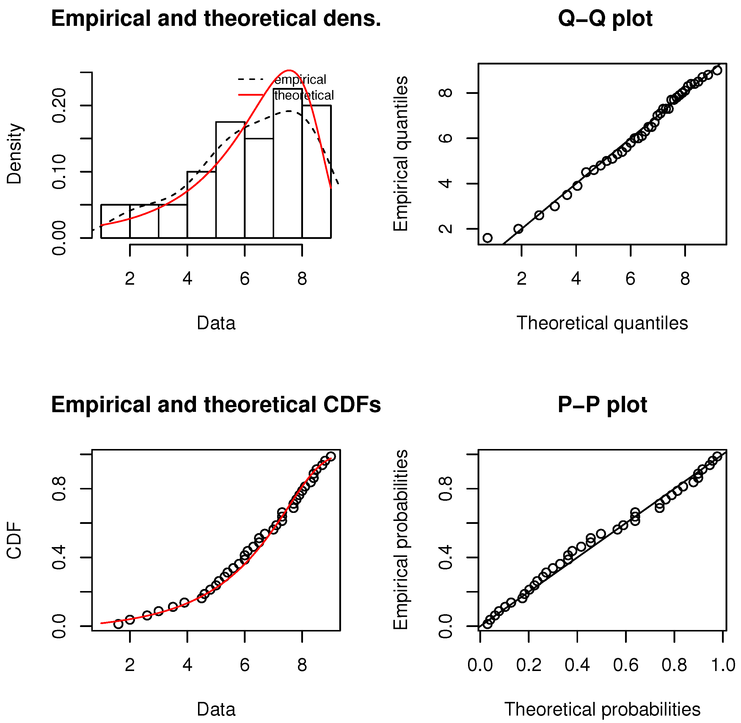
Table 2 and Table 3 present the maximum likelihood estimates, with the corresponding standard errors in parentheses, of the unknown parameters ($\lambda ,\alpha ,a,b,c$) of the MBGz distribution for Datasets 1 and 2, respectively. Table 4 and Table 5 show the statistics AIC, BIC, W*, A*, KS, and p-Value values for all the considered models. We then see that the proposed MBGz model fits the considered data better than the other models. Thus, the proposed MBGz model provides an interesting alternative to other existing models for modeling positive real data. To complete this fact, PP, QQ, epdf and ecdf plots of the MBGz distribution are given in Figure 2 and Figure 3 for Datasets 1 and 2, respectively.

Table 2. MLEs (standard errors in parentheses) for Dataset 1.

Distribution			Estimates
MBGz ($\lambda ,\alpha ,a,b,c$)	0.0085	2.5537	1.0737	1.3153	5.0687
	(0.0067)	(0.5727)	(0.3197)	(0.8933)	(3.3003)
EGWGz ($\lambda ,a,b,c,\beta$)	3.2078	2.4598	0.0203	1.8974	0.5460
	(1.2099)	(0.6498)	(0.0531)	(1.8193)	(0.2430)
KwGz ($a,b,c,d,\theta$)	0.1861	1.4948	1.4909	0.9811
	(0.3130)	(0.5076)	(0.4735)	(2.4368)
BGz ($a,b,\theta ,v$)	0.3144	1.5591	1.4798	0.4966
	(0.4283)	(0.3658)	(0.4543)	(0.8692)
Gz ($\lambda ,\alpha$)	0.0841	1.8811
	(0.0268)	(0.2043)

Table 3. MLEs (standard errors in parentheses) for Dataset 2.

Distribution			Estimates
MBGz ($\lambda ,\alpha ,a,b,c$)	0.0098	0.5270	0.8768	4.5635	0.1561
	(0.0116)	(0.1599)	(0.3893)	(0.8862)	(0.2442)
EGWGz ($\lambda ,a,b,c,\beta$)	0.0101	0.6077	0.1078	1.6929	0.6613
	(0.0141)	(0.1506)	(0.3427)	(1.2539)	(0.3379)
KwGz ($a,b,\theta ,v$)	0.0133	0.2923	2.0164	13.7085
	(0.0120)	(0.1641)	(0.7880)	(7.0208)
BGz ($a,b,c,d,\theta$)	0.0125	0.1856	3.7622	2.0116
	(0.0100)	(0.1601)	(2.5635)	(3.3802)
Gz ($\lambda ,\alpha$)	0.0074)	(0.6243)
	(0.0035)	(0.0748)

Table 4. The AIC, BIC, W*, A*, KS, and p-Value values for Dataset 1.

Dist	$\widehat{\ell }$	AIC	BIC	W*	A*	KS	p-Value
MBGz	50.0387	110.0776	118.2481	0.0328	0.2745	0.0539	0.9889
EGWGz	52.6888	115.3776	126.5482	0.0706	0.5341	0.0785	0.7885
KwGz	51.2042	110.4084	119.3448	0.0529	0.4125	0.0640	0.9396
BGz	51.1518	110.3026	119.2399	0.0518	0.4057	0.0627	0.9484
Gz	53.9686	111.9374	122.4056	0.0819	0.5921	0.0810	0.7547

Table 5. The AIC, BIC, W*, A*, KS, and p-Value values for Dataset 2.

Dist	$\widehat{\ell }$	AIC	BIC	W*	A*	KS	p-Value
MBGz	78.2184	168.1770	176.0214	0.0222	0.1840	0.0707	0.9888
EGWGz	79.3744	168.5489	178.5933	0.0479	0.2922	0.0821	0.9623
KwGz	80.7197	169.4395	176.1950	0.0430	0.3326	0.0966	0.8489
BGz	82.9924	173.9849	180.7404	0.0922	0.6736	0.1080	0.7389
Gz	80.9566	168.9234	177.2911	0.0359	0.2335	0.0903	0.8299

Figure 2. PP, QQ, epdf and ecdf plots of the MBGz distribution for Dataset 1.

Figure 3. PP, QQ, epdf and ecdf plots of the MBGz distribution for Dataset 2.

References

- Gompertz, B. On the nature of the function expressive of the law of human mortality and on the new mode of determining the value of life contingencies. Philos. Trans. R. Soc. A 1825, 115, 513–580. [Google Scholar] [CrossRef]
- Tjørve, K.M.C.; Tjørve, E. The use of Gompertz models in growth analyses, and new Gompertz-model approach: An addition to the Unified-Richards family. PLoS ONE 2017, 12. [Google Scholar] [CrossRef]
- El-Gohary, A.; Alshamrani, A.; Al-Otaibi, A. The generalized Gompertz distribution. Appl. Math. Model. 2013, 37, 13–24. [Google Scholar] [CrossRef]
- Jafari, A.A.; Tahmasebi, S.; Alizadeh, M. The beta-Gompertz distribution. Revista Colombiana de Estadistica 2014, 37, 141–158. [Google Scholar] [CrossRef]
- Eugene, N.; Lee, C.; Famoye, F. Beta-normal distribution and its applications. Comm. Statist. Theory Methods 2002, 31, 497–512. [Google Scholar] [CrossRef]
- Benkhelifa, L. The beta generalized Gompertz distribution. Appl. Math. Model. 2017, 52, 341–357. [Google Scholar] [CrossRef]
- El-Damcese, M.A.; Mustafa, A.; El-Desouky, B.S.; Mustafa, M.E. Generalized Exponential Gompertz Distribution. Appl. Math. 2015, 6, 2340–2353. [Google Scholar] [CrossRef]
- Tahir, M.H.; Cordeiro, G.M.; Alizadeh, M.; Mansoor, M.; Zubair, M.; Hamedani, G.G. The Odd Generalized Exponential Family of Distributions with Applications. J. Stat. Distrib. Appl. 2015, 2, 1–28. [Google Scholar] [CrossRef]
- Roozegar, R.; Tahmasebi, S.; Jafari, A.A. The McDonald Gompertz distribution: Properties and applications. Commun. Stat. Simul. Comput. 2017, 46, 3341–3355. [Google Scholar] [CrossRef]
- Alexander, C.; Cordeiro, G.M.; Ortega, E.M.M.; Sarabia, J.M. Generalized beta-generated distributions. Comput. Stat. Data Anal. 2012, 56, 1880–1897. [Google Scholar] [CrossRef]
- Khan, M.S.; King, R.; Hudson, I.L. Transmuted Generalized Gompertz distribution with application. J. Stat. Theory Appl. 2017, 16, 65–80. [Google Scholar] [CrossRef]
- Moniem, A.I.B.; Seham, M. Transmuted Gompertz Distribution. Comput. Appl. Math. 2015, 1, 88–96. [Google Scholar]
- Shaw, W.; Buckley, I. The Alchemy of Probability Distributions: Beyond Gram-Charlier Expansions and a Skewkurtotic-Normal Distribution from a Rank Transmutation Map; Research Report; King’s College: London, UK, 2007. [Google Scholar]
- Chukwu, A.U.; Ogunde, A.A. On kumaraswamy gompertz makeham distribution. Am. J. Math. Stat. 2016, 6, 122–127. [Google Scholar]
- Lima, F.P.; Sanchez, J.D.; da Silva, R.C.; Cordeiro, G.M. The Kumaraswamy Gompertz distribution. J. Data Sci. 2015, 13, 241–260. [Google Scholar]
- Benkhelifa, L. Marshall-Olkin extended generalized Gompertz distribution. J. Data Sci. 2017, 15, 239–266. [Google Scholar]
- Yaghoobzadeh, S. A new generalization of the Marshall-Olkin Gompertz distribution. Int. J. Syst. Assur. Eng. Manag. 2017, 8, 1580–1587. [Google Scholar] [CrossRef]
- Marshall, A.W.; Olkin, I. A new method for adding a parameter to a family of distributions with application to the exponential and Weibull families. Biometrika 1997, 84, 641–652. [Google Scholar] [CrossRef]
- Shadrokh, A.; Yaghoobzadeh, S.S. The Beta Gompertz Geometric Distribution: Mathematical Properties and Applications. Andishe_ye Amari 2018, 22, 81–91. [Google Scholar]
- Nadarajah, S.; Teimouri, M.; Shih, S.H. Modified Beta Distributions. Sankhya Ser. B 2014, 76, 19–48. [Google Scholar] [CrossRef]
- Alizadeh, M.; Cordeiro, G.M.; Brito, E. The beta Marshall-Olkin family of distributions. J. Stat. Distrib. Appl. 2015, 2, 4. [Google Scholar] [CrossRef]
- Nadarajah, S.; Kotz, S. The beta exponential distribution. Reliab. Eng. Syst. Saf. 2006, 91, 689–697. [Google Scholar] [CrossRef]
- Gupta, R.D.; Kundu, D. Generalized Exponential Distributions. Aust. N. Z. J. Stat. 1999, 41, 173–188. [Google Scholar] [CrossRef]
- Kenney, J.F.; Keeping, E.S. Mathematics of Statistics, 3rd ed.; Chapman and Hall Ltd.: Rahway, NJ, USA, 1962. [Google Scholar]
- Moors, J.J. A quantile alternative for kurtosis. J. R. Stat. Soc. Ser. D 1988, 37, 25–32. [Google Scholar] [CrossRef]
- Milgram, M. The generalized integro-exponential function. Math. Comput. 1985, 44, 443–458. [Google Scholar] [CrossRef]
- Lenart, A. The moments of the Gompertz distribution and maximum likelihood estimation of its parameters. Scand. Actuar. J. 2014, 3, 255–277. [Google Scholar] [CrossRef]
- MacGillivray, H.L. Skewness and Asymmetry: Measures and Orderings. Ann. Stat. 1986, 14, 994–1011. [Google Scholar] [CrossRef]
- Gradshteyn, I.S.; Ryzhik, I.M. Table of Integrals, Series and Products; Academic Press: New York, NY, USA, 2000. [Google Scholar]
- El-Bassiouny, H.; EL-Damcese, M.; Mustafa, A.; Eliwa, M.S. Exponentiated Generalized Weibull-Gompertz Distribution with Application in Survival Analysis. J. Stat. Appl. Probab. 2017, 6, 7–16. [Google Scholar] [CrossRef]
- Xu, K.; Xie, M.; Tang, L.C.; Ho, S.L. Application of Neural Networks in forecasting Engine Systems Reliability. Appl. Soft Comput. 2003, 2, 255–268. [Google Scholar] [CrossRef]
- Badar, M.G.; Priest, A.M. Statistical aspects of fiber and bundle strength in hybrid composites. In Progress in Science and Engineering Composites, Proceedings of the ICCM-IV, Tokyo, Japan, 25–28 October 1982; Hayashi, T., Kawata, K., Umekawa, S., Eds.; Japan Society for Composite Materials: Tokyo, Japan, 1982; pp. 1129–1136. [Google Scholar]
Figure 1.
Some plots of the pdf (a); and some plots for the hrf (b).
Figure 2.
PP, QQ, epdf and ecdf plots of the MBGz distribution for Dataset 1.
Figure 3.
PP, QQ, epdf and ecdf plots of the MBGz distribution for Dataset 2.