Generic Properties of Framed Rectifying Curves

Abstract

The position vectors of regular rectifying curves always lie in their rectifying planes. These curves were well investigated by B.Y.Chen. In this paper, the concept of framed rectifying curves is introduced, which may have singular points. We investigate the properties of framed rectifying curves and give a method for constructing framed rectifying curves. In addition, we reveal the relationships between framed rectifying curves and some special curves.

1. Introduction

Curves, which are the basic objects of study, have attracted much attention from many mathematicians and physicists [1,2,3]. Due to the need to observe the properties of special curves, a renewed interest in curves has developed, such as rectifying curves in different spaces. The space curves whose position vectors always lie in their rectifying planes are called rectifying curves. B.Y. Chen gave the notion of rectifying curves in [4]. In [5], the relationship between centrodes of space curves and rectifying curves was revealed by F. Dillen and B.Y. Chen. In kinematics, the centrode is the path traced by the instantaneous center of rotation of a rigid plane figure moving in a plane, and it has wide applications in mechanics and joint kinematics (see [6,7,8,9]).

Since B.Y. Chen’s important work, the notion of rectifying curves was extended to other ambient spaces [10,11,12,13]. As we know, regular curves determine the curvature functions and torsion functions, which can provide valuable geometric information about the curves by the Frenet frames of the original curves. If space curves have singular points, the Frenet frames of these curves cannot be constructed. However, S. Honda and M. Takahashi [14] gave the definition of framed curves. Framed curves are space curves with moving frames, and they may have singular points. They are the generalizations of not only Legendrian curves in unit tangent bundles, but also regular curves with linear independent conditions (see [15]).

Inspired by the above work, in order to investigate the properties of rectifying curves with singular points, we should give the concept of framed rectifying curves. The difficulties arise because tangent vectors vanish at singular points, so it is impossible to normalize tangent vectors, principal normal vectors, and binormal vectors in the usual way. Here, we define the generalized tangent vector, the generalized principle normal vector, and the generalized binormal vector, respectively. Actually, at regular points, they are just the usual tangent vector, principle vector, and binormal vector. We obtain moving adapted frames for framed rectifying curves, and some smooth functions similar to the curvature of regular curves are defined by using moving adapted frames. These functions are referred to as framed curvature, which is very useful to analyze framed rectifying curves. On this basis, we investigate the properties of framed rectifying curves and give some sufficient and necessary conditions for the judgment of framed rectifying curves. Moreover, we give a method for constructing framed rectifying curves. In this paper, framed helices are also defined. We discuss the relationship between framed rectifying curves and framed helices in terms of the ratio of framed curvature. In particular, the ratio of framed curvature for framed rectifying curves has extrema at singular points. In addition, we give the notions of the centrodes of the framed curves and circular rectifying curves and reveal the relationships between framed rectifying curves and these special curves.

The organization of this paper is as follows. We review the concept of the framed curve and define an adapted frame and framed curvature for the framed curve in Section 2. We provide some sufficient and necessary conditions for the judgment of framed rectifying curves in Section 3. An important result, which explicitly determines all framed rectifying curves, is given in Section 4. Moreover, the relationships between framed rectifying curves and framed helices and framed rectifying curves and centrodes are given in Section 5 and Section 6, respectively. At last, we consider the contact between framed rectifying curves and model curves (circular rectifying curves) in Section 7.

2. Framed Curve and Adapted Frame

Let ${\mathbb{R}}^3$ be the three-dimensional Euclidean space, and let $\gamma :I\to {\mathbb{R}}^3$ be a curve with singular points. In order to investigate this curve, we will introduce the framed curve (cf., [14]). We denote the set ${\Delta }_2$ as follows:

$$\begin{array}{c}\hfill {\Delta }_2=\{\mathbf{\mu }=({\mathbf{\mu }}_1,{\mathbf{\mu }}_2)\in {\mathbb{R}}^3\times {\mathbb{R}}^3|{\mathbf{\mu }}_i·{\mathbf{\mu }}_j={\delta }_{ij},i,j=1,2\}.\end{array}$$

Then, ${\Delta }_2$ is a three-dimensional smooth manifold. Let $\mathit{\mu }=({\mathit{\mu }}_1,{\mathit{\mu }}_2)\in {\Delta }_2.$ We define a unit vector $\mathit{\nu }={\mathit{\mu }}_1\times {\mathit{\mu }}_2$ in ${\mathbb{R}}^3.$ This means that $\mathit{\nu }$ is orthogonal to ${\mathit{\mu }}_1$ and ${\mathit{\mu }}_2.$

Definition 1.

We say that $(\mathit{\gamma },\mathit{\mu }):I\to {\mathbb{R}}^3\times {\Delta }_2$ is a framed curve if $⟨{\mathit{\gamma }}^{\prime }(s),{\mathit{\mu }}_i(s)⟩=0$ for all $s\in I$ and $i=1,2.$ We also say that $\mathit{\gamma }:I\to {\mathbb{R}}^3$ is a framed base curve if there exists $\mathit{\mu }:I\to {\Delta }_2$ such that $(\mathit{\gamma },\mathit{\mu })$ is a framed curve.

Let $(\mathit{\gamma },{\mathit{\mu }}_1,{\mathit{\mu }}_2):I\to {\mathbb{R}}^3\times {\Delta }_2$ be a framed curve and $\mathit{\nu }(s)={\mathit{\mu }}_1(s)\times {\mathit{\mu }}_2(s).$ Then, we have the following Frenet–Serret formula:

$$\left\{\begin{array}{c}{\mathit{\mu }}_1^{\prime }(s)=l(s){\mathit{\mu }}_2(s)+m(s)\mathit{\nu }(s)\hfill \\ {\mathit{\mu }}_2^{\prime }(s)=-l(s){\mathit{\mu }}_1(s)+n(s)\mathit{\nu }(s)\hfill \\ {\mathit{\nu }}^{\prime }(s)=-m(s){\mathit{\mu }}_1(s)-n(s){\mathit{\mu }}_2(s).\hfill \end{array}\right.$$

Here, $l(s)=⟨{\mathit{\mu }}_1^{\prime }(s),{\mathit{\mu }}_2(s)⟩,$ $m(s)=⟨{\mathit{\mu }}_1^{\prime }(s),\mathit{\nu }(s)⟩$ and $n(s)=⟨{\mathit{\mu }}_2^{\prime }(s),\mathit{\nu }(s)⟩.$ In addition, there exists a smooth mapping $\alpha :I\to \mathbb{R}$ such that:

$$\begin{array}{c}\hfill {\gamma }^{\prime }(s)=\alpha (s)\mathbf{\nu }(s).\end{array}$$

The four functions $(l(s),m(s),n(s),\alpha (s))$ are called the curvature of $\mathit{\gamma }$. If $m(s)=n(s)=0,$ then ${\mathit{\nu }}^{\prime }(s)=\mathbf{0}.$ In this paper, we consider the case ${\mathit{\nu }}^{\prime }(s)\ne \mathbf{0}.$ Obviously, $\alpha (s_0)=0$ if and only if $s_0$ is a singular point of $\gamma$. We can use the curvature of the framed curve to analyze the singular points.

In [14], the theorems of the existence and uniqueness for framed curves were shown as follows:

Theorem 1.

Let $(l,m,n,\alpha ):I\to {\mathbb{R}}^4$ be a smooth mapping. There exists a framed curve $(\mathit{\gamma },\mathit{\mu }):I\to {\mathbb{R}}^3\times {\Delta }_2$ whose associated curvature of the framed curve is $(l,m,n,\alpha ).$

Theorem 2.

Let $(\mathit{\gamma },\mathit{\mu })$ and $(\overline{\mathit{\gamma }},\overline{\mathit{\mu }}):I\to {\mathbb{R}}^3\times {\Delta }_2$ be framed curves whose curvatures of the framed curves $(l,m,n,\alpha )$ and $(\overline{l},\overline{m},\overline{n},\overline{\alpha })$ coincide. Then, $(\mathit{\gamma },\mathit{\mu })$ and $(\overline{\mathit{\gamma }},\overline{\mathit{\mu }})$ are congruent as framed curves.

Let $(\mathit{\gamma },{\mathit{\mu }}_1,{\mathit{\mu }}_2):I\to {\mathbb{R}}^3\times {\Delta }_2$ be a framed curve with the curvature $(l(s),m(s),n(s),\alpha (s)).$ ${\mathit{\mu }}_1$ and ${\mathit{\mu }}_2$ are the base vectors of the normal plane of $\mathit{\gamma }(s)$, as a case similar to the Bishop frame for regular curves [16]. We define $({\overline{\mathit{\mu }}}_1,{\overline{\mathit{\mu }}}_2)\in {\Delta }_2$ by:

$$\left(\begin{array}{c}{\overline{\mathit{\mu }}}_1(s)\\ {\overline{\mathit{\mu }}}_2(s)\end{array}\right)=\left(\begin{array}{cc}cos\theta (s)& -sin\theta (s)\\ sin\theta (s)& cos\theta (s)\end{array}\right)\left(\begin{array}{c}{\mathit{\mu }}_1(s)\\ {\mathit{\mu }}_2(s)\end{array}\right).$$

Here, $\theta (s)$ is a smooth function. Obviously, $(\mathit{\gamma },{\overline{\mathit{\mu }}}_1,{\overline{\mathit{\mu }}}_2)\to {\mathbb{R}}^3\times {\Delta }_2$ is also a framed curve, and we have:

$$\begin{array}{c}\hfill \overline{\mathbf{\nu }}(s)={\mathbf{\mu }}_1(s)\times {\mathbf{\mu }}_2(s)={\overline{\mathbf{\mu }}}_1(s)\times {\overline{\mathbf{\mu }}}_2(s)=\mathbf{\nu }(s).\end{array}$$

By straightforward calculations, we have:

$$\begin{array}{cc}\hfill {\overline{\mathbf{\mu }}}_1^{\prime }(s)=& (l(s)-{\theta }^{\prime }(s))sin\theta (s){\mathbf{\mu }}_1(s)+(l(s)-{\theta }^{\prime }(s))cos\theta (s){\mathbf{\mu }}_2(s)\hfill \\ & +(m(s)cos\theta (s)-n(s)sin\theta (s))\mathbf{\nu }(s),\hfill \end{array}$$

$$\begin{array}{cc}\hfill {\overline{\mathbf{\mu }}}_2^{\prime }(s)=& -(l(s)-{\theta }^{\prime }(s))cos\theta (s){\mathbf{\mu }}_1(s)+(l(s)-{\theta }^{\prime }(s))sin\theta (s){\mathbf{\mu }}_2(s)\hfill \\ & +(m(s)sin\theta (s)+n(s)cos\theta (s))\mathbf{\nu }(s).\hfill \end{array}$$

Let $\theta :I\to \mathbb{R}$ be a smooth function that satisfies $m(s)sin\theta (s)=-n(s)cos\theta (s).$ Assume that $m(s)=-p(s)cos\theta (s),$ $n(s)=p(s)sin\theta (s),$ then we have:

$$\begin{array}{c}\hfill {\mathbf{\nu }}^{\prime }(s)=-m(s){\mathbf{\mu }}_1(s)-n(t){\mathbf{\mu }}_2(s)=p(s)(cos\theta (s){\mathbf{\mu }}_1(s)-sin\theta (s){\mathbf{\mu }}_2(s))=p(s){\overline{\mathbf{\mu }}}_1(s),\end{array}$$

$$\begin{array}{cc}\hfill {\overline{\mathbf{\mu }}}_1^{\prime }(s)=& (l(s)-{\theta }^{\prime }(s))sin\theta (s){\mathbf{\mu }}_1(s)+(l(s)-{\theta }^{\prime }(s))cos\theta (s){\mathbf{\mu }}_2(s)+(m(s)cos\theta (s)-n(s)sin\theta (s))\mathbf{\nu }(s)\hfill \\ \hfill =& -p(s)\mathbf{\nu }(s)+(l(s)-{\theta }^{\prime }(s)){\overline{\mathbf{\mu }}}_2(s)\hfill \end{array}$$

and:

$$\begin{array}{cc}\hfill {\overline{\mathbf{\mu }}}_2^{\prime }(s)=& -(l(s)-{\theta }^{\prime }(s))cos\theta (s){\mathbf{\mu }}_1(s)+(l(s)-{\theta }^{\prime }(s))sin\theta (s){\mathbf{\mu }}_2(s)+(m(s)sin\theta (s)+n(s)cos\theta (s))\mathbf{\nu }(s)\hfill \\ \hfill =& -(l(s)-{\theta }^{\prime }(s)){\overline{\mathbf{\mu }}}_1(s).\hfill \end{array}$$

The vectors $\mathit{\nu }(s),{\overline{\mathit{\mu }}}_1(s),{\overline{\mathit{\mu }}}_2(s)$ form an adapted frame along $\mathit{\gamma }(s)$, and we have the following Frenet–Serret formula:

$$\left(\begin{array}{c}{\mathit{\nu }}^{\prime }(s)\\ {\overline{\mathit{\mu }}}_1^{\prime }(s)\\ {\overline{\mathit{\mu }}}_2^{\prime }(s)\end{array}\right)=\left(\begin{array}{ccc}0& p(s)& 0\\ -p(s)& 0& q(s)\\ 0& -q(s)& 0\end{array}\right)\left(\begin{array}{c}\mathit{\nu }(s)\\ {\overline{\mathit{\mu }}}_1(s)\\ {\overline{\mathit{\mu }}}_2(s)\end{array}\right).$$

We call the vectors $\mathit{\nu }(s),{\overline{\mathit{\mu }}}_1(s),{\overline{\mathit{\mu }}}_2(s)$ the generalized tangent vector, the generalized principle normal vector, and the generalized binormal vector of the framed curve, respectively, where $p(s)=|{\mathit{\nu }}^{\prime }(s)|>0$ and $q(s)=l(s)-{\theta }^{\prime }(s).$ The functions $(p(s),q(s),\alpha (s))$ are referred to as the framed curvature of $\mathit{\gamma }(s)$.

Proposition 1.

Let $(\mathit{\gamma },{\overline{\mathit{\mu }}}_1,{\overline{\mathit{\mu }}}_2):I\to {\mathbb{R}}^3\times {\Delta }_2$ be a framed curve. The relationships among the curvature $\kappa (s)$, the torsion $\tau (s)$, and the framed curvature $(p(s),q(s),\alpha (s))$ of a regular curve are given by:

$$\begin{array}{c}\hfill \kappa (s)=\frac{p(s)}{|\alpha (s)|},\tau (s)=\frac{q(s)}{\alpha (s)}.\end{array}$$

Proof. 

By straightforward calculations, we have:

$$\begin{array}{c}\hfill {\mathbf{\gamma }}^{\prime }(s)=\alpha (s)\mathbf{\nu }(s),\end{array}$$

$$\begin{array}{c}\hfill {\mathbf{\gamma }}^{″}(s)={\alpha }^{\prime }(s)\mathbf{\nu }(s)+\alpha (s)p(s){\overline{\mathbf{\mu }}}_1(s),\end{array}$$

$$\begin{array}{c}\hfill {\mathbf{\gamma }}^{‴}(s)=({\alpha }^{″}(s)-\alpha (s)p^2(s))\mathbf{\nu }(s)+(2{\alpha }^{\prime }(s)p(s)+\alpha (t)p^{\prime }(s)){\overline{\mathbf{\mu }}}_1(s)+\alpha (s)p(s)q(s){\overline{\mathbf{\mu }}}_2(s).\end{array}$$

It follows:

$$\begin{array}{c}\hfill |{\mathbf{\gamma }}^{\prime }(s)|=|\alpha (s)|,\end{array}$$

$$\begin{array}{c}\hfill |{\mathbf{\gamma }}^{\prime }(s)\times {\mathbf{\gamma }}^{″}(s)|={\alpha }^2(s)p(s),\end{array}$$

$$\begin{array}{c}\hfill \det ({\mathbf{\gamma }}^{\prime }(s),{\mathbf{\gamma }}^{″}(s),{\mathbf{\gamma }}^{‴}(s))={\alpha }^3(s)p^2(s)q(s).\end{array}$$

Therefore, the relationships are shown by:

$$\begin{array}{c}\hfill \kappa (s)=\frac{|{\mathbf{\gamma }}^{\prime }(s)\times {\mathbf{\gamma }}^{″}(s)|}{|{\mathbf{\gamma }}^{\prime }{(s)|}^3}=\frac{p(s)}{|\alpha (s)|},\end{array}$$

$$\begin{array}{c}\hfill \tau (s)=\frac{\det ({\mathbf{\gamma }}^{\prime }(s),{\mathbf{\gamma }}^{″}(s),{\mathbf{\gamma }}^{‴}(s))}{|{\mathbf{\gamma }}^{\prime }(s)\times {\mathbf{\gamma }}^{\prime \prime }{(s)|}^2}=\frac{q(s)}{\alpha (s)}.\end{array}$$

☐

3. Framed Rectifying Curves

In this section, the framed rectifying curves are defined, and we investigate their properties.

Definition 2.

Let $(\mathit{\gamma },{\overline{\mathit{\mu }}}_1,{\overline{\mathit{\mu }}}_2):I\to {\mathbb{R}}^3\times {\Delta }_2$ be a framed curve. We call $\mathit{\gamma }$ a framed rectifying curve if its position vector $\mathit{\gamma }$ satisfies:

$$\begin{array}{c}\hfill \mathbf{\gamma }(s)=\lambda (s)\mathbf{\nu }(s)+\xi (s){\overline{\mathbf{\mu }}}_2(s)\end{array}$$

for some functions $\lambda (s)$ and $\xi (s).$

Some properties of the framed rectifying curves are shown in the following theorem.

Theorem 3.

Let $(\mathit{\gamma },{\overline{\mathit{\mu }}}_1,{\overline{\mathit{\mu }}}_2):I\to {\mathbb{R}}^3\times {\Delta }_2$ be a framed curve with $p(s)>0$. The following statements are equivalent.

(i) The relation between the framed curvature and the framed curve is as follows:

$$\begin{array}{c}\hfill {⟨\mathbf{\gamma }(s),\mathbf{\nu }(s)⟩}^{\prime }=\alpha (s).\end{array}$$

(ii) The distance squared function satisfies $f(s)=⟨\mathit{\gamma }(s),\mathit{\gamma }(s)⟩={⟨\mathit{\gamma }(s),\mathit{\nu }(s)⟩}^2+C$ for some positive constant $C.$

(iii) $⟨\mathit{\gamma }(s),{\overline{\mathit{\mu }}}_2(s)⟩=\xi ,$ ξ is a constant.

(iv) $\mathit{\gamma }(s)$ is a framed rectifying curve.

Proof. 

Let $\mathit{\gamma }(s)$ be a framed rectifying curve. By definition, there exist some functions $\lambda (s)$ and $\xi (s)$ such that:

$$\begin{array}{c}\hfill \mathbf{\gamma }(s)=\lambda (s)\mathbf{\nu }(s)+\xi (s){\overline{\mathbf{\mu }}}_2(s).\end{array}$$

(1)

By using the Frenet–Serret formula and taking the derivative of (1) with respect to s, we have:

$$\begin{array}{c}\hfill {\lambda }^{\prime }(s)=\alpha (s),\lambda (s)p(s)=\xi (s)q(s),{\xi }^{\prime }(s)=0.\end{array}$$

(2)

From the first and third equalities of (2), we have that ${⟨\mathit{\gamma }(s),\mathit{\nu }(s)⟩}^{\prime }={\lambda }^{\prime }(s)=\alpha (s).$ This proves Statement (i). Since ${\xi }^{\prime }(s)=0,$ we can obtain Statement (iii). From (1) and (2), we have that $⟨\mathit{\gamma }(s),\mathit{\gamma }(s)⟩={\lambda }^2(s)+{\xi }^2={⟨\mathit{\gamma }(s),\mathit{\nu }(s)⟩}^2+C,$ $C={\xi }^2$ is positive. This proves Statement (ii).

Conversely, let us assume that Statement (i) holds.

$$\begin{array}{c}\hfill {⟨\mathbf{\gamma }(s),\mathbf{\nu }(s)⟩}^{\prime }=⟨\alpha (s)\mathbf{\nu }(s),\mathbf{\nu }(s)⟩+p(s)⟨\mathbf{\gamma }(s),{\overline{\mathbf{\mu }}}_1(s)⟩=\alpha (s).\end{array}$$

Since $p(s)>0$, by assumption, we have $⟨\mathit{\gamma }(s),{\overline{\mathit{\mu }}}_1(s)⟩=0.$ This means the curve is a framed rectifying curve.

If Statement (ii) holds, $⟨\mathit{\gamma }(s),\mathit{\gamma }(s)⟩={⟨\mathit{\gamma }(s),\mathit{\nu }(s)⟩}^2+C,$ where C is a positive constant. Then, we have:

$$\begin{array}{c}\hfill 2⟨\mathbf{\gamma }(s),\alpha (s)\mathbf{\nu }(s)⟩=2⟨\mathbf{\gamma }(s),\mathbf{\nu }(s)⟩(\alpha (s)+p(s)⟨\mathbf{\gamma }(s),{\overline{\mathbf{\mu }}}_1(s)⟩)\end{array}$$

and $⟨\mathit{\gamma }(s),{\overline{\mathit{\mu }}}_1(s)⟩=0.$ Therefore, $\mathit{\gamma }(s)$ is a framed rectifying curve. Statement (iii) implies that the curve is a framed rectifying curve by an appeal to the Frenet–Serret formula. ☐

Remark 1.

$s_0$ is a singular point of the framed rectifying curve $\mathit{\gamma }$ if and only if $\alpha (s_0)=0.$ From (2) and Statement (ii), we know that the ratio $q(s)/p(s)$ and the distance squared function $f(s)$ have extrema at $s_0.$

4. Construction Approach of Framed Rectifying Curves

In [4], the construction approach of regular rectifying curves is given by B. Y. Chen in Theorem 3, but it is not suitable for the non-regular case. In this section, a new construction approach is provided, which can be applied to both regular rectifying curves and non-regular rectifying curves. Moreover, it explicitly determines all framed rectifying curves in Euclidean three-space. First, we introduce the notion of the framed spherical curve.

Definition 3.

Let $(\mathit{\gamma },{\overline{\mathit{\mu }}}_1,{\overline{\mathit{\mu }}}_2):I\to {\mathbb{R}}^3\times {\Delta }_2$ be a framed curve. We call $\mathit{\gamma }$ a framed spherical curve if the framed base curve $\mathit{\gamma }$ is a curve on $S^2$.

We show the key theorem in this section as follows.

Theorem 4.

Let $(\mathit{\gamma },{\overline{\mathit{\mu }}}_1,{\overline{\mathit{\mu }}}_2):I\to {\mathbb{R}}^3\times {\Delta }_2$ be a framed curve with $p(s)>0.$ Then, $\mathit{\gamma }$ is a framed rectifying curve if and only if:

$$\begin{array}{c}\hfill \mathbf{\gamma }(s)=\rho ({tan}^2(\int |{\mathit{g}}^{\prime }{(s)|ds+C)+1)}^{\frac{1}{2}}\mathit{g}(s),\end{array}$$

(3)

where C is a constant, ρ is a positive number, and $\mathit{g}(s)$ is a framed spherical curve.

Proof. 

Let $\mathit{\gamma }$ be a framed rectifying curve. From Theorem 3, we have $⟨\mathit{\gamma }(s),\mathit{\gamma }(s)⟩={\lambda }^2(s)+{\rho }^2,$ where $\rho$ is a positive number. The framed rectifying curve $\mathit{\gamma }(s)$ can be written as:

$$\begin{array}{c}\hfill \mathbf{\gamma }(s)={({\lambda }^2(s)+{\rho }^2)}^{\frac{1}{2}}\mathit{g}(s),\end{array}$$

(4)

where $\mathit{g}(s)$ is a framed spherical curve. By taking the derivative of (4), we have:

$$\begin{array}{c}\hfill {\mathbf{\gamma }}^{\prime }(s)=\frac{\lambda (s)\alpha (s)}{{({\lambda }^2(s)+{\rho }^2)}^{\frac{1}{2}}}\mathit{g}(s)+{({\lambda }^2(s)+{\rho }^2)}^{\frac{1}{2}}{\mathit{g}}^{\prime }(s).\end{array}$$

(5)

As ${\mathit{\gamma }}^{\prime }(s)=\alpha (s)\mathit{\nu }(s),$ ${\mathit{g}}^{\prime }(s)$ is orthogonal to $\mathit{g}(s).$ Therefore, Equality (5) implies:

$$\begin{array}{c}\hfill |{\mathit{g}}^{\prime }(s)|=|\frac{\rho \alpha (s)}{{\lambda }^2(s)+{\rho }^2}|,\end{array}$$

and we have

$$\begin{array}{c}\hfill \int |{\mathbf{\gamma }}^{\prime }(s)|ds+C=arctan(\frac{\lambda (s)}{\rho }).\end{array}$$

Then, $\lambda (s)=\rho tan(\int |{\mathit{g}}^{\prime }(s)|ds+C),$ and substituting this equality into (4) yields (3).

Conversely, assume $\mathit{\gamma }(s)$ is a framed curve defined by:

$$\begin{array}{c}\hfill \mathbf{\gamma }(s)=\rho ({tan}^2(\int |{\mathit{g}}^{\prime }{(s)|ds+C)+1)}^{\frac{1}{2}}\mathit{g}(s)\end{array}$$

(6)

for a constant C, a positive number $\rho$, and a framed curve $\mathit{g}(s)$ on $S^2.$ Let $\tilde{\lambda }(s)=\rho tan(\int |{\mathit{g}}^{\prime }(s)|ds+C)$ and ${\tilde{\lambda }}^{\prime }(s)={\tilde{\alpha }}^{\prime }(s).$ Then, $\int |{\mathit{g}}^{\prime }(s)|ds+C=arctan(\frac{\widetilde{\lambda (s)}}{\rho }).$ By taking the derivative of this equality, we get:

$$\begin{array}{c}\hfill \frac{\rho \tilde{\alpha }(s)}{{\tilde{\lambda }}^2(s)+{\rho }^2}=|{\mathit{g}}^{\prime }(s)|\end{array}$$

(7)

and:

$$\begin{array}{c}\hfill {\mathbf{\gamma }}^{\prime }(s)=\frac{\tilde{\lambda }(s)\tilde{\alpha }(s)}{{({\tilde{\lambda }}^2(s)+{\rho }^2)}^{\frac{1}{2}}}\mathit{g}(s)+{({\tilde{\lambda }}^2(s)+{\rho }^2)}^{\frac{1}{2}}{\mathit{g}}^{\prime }(s).\end{array}$$

(8)

Equality (7) and Equality (8) imply that $|{\mathit{g}}^{\prime }(s)|=\tilde{\alpha }(s),$ since ${\mathit{g}}^{\prime }(s)=\lambda (s)\mathit{\nu }(s).$ We have $\tilde{\alpha }(s)=\pm \lambda (s),$ $\tilde{\lambda }(s)=\pm \lambda (s).$ Then:

$$\begin{array}{c}\hfill \mathbf{\gamma }(s)={({\lambda }^2(s)+{\rho }^2)}^{\frac{1}{2}}\mathit{g}(s),\end{array}$$

(9)

which shows that the distance squared function satisfies Statement (ii) in Theorem 3. It follows that $\mathit{\gamma }(s)$ is a framed rectifying curve. ☐

Framed rectifying curves include regular rectifying curves and non-regular rectifying curves. We will give two examples.

Example 1.

Let ${\mathit{g}}_1(s)=(\frac{1}{2}cos2s,\frac{1}{2}sin2s,\frac{\sqrt{3}}{2}),$ $s\in (-\frac{\pi }{2},\frac{\pi }{2}),$ then ${\mathit{g}}_1(s)$ is a space curve on $S^2.$ We have $|{\mathit{g}}_1^{\prime }(s)|=1.$ Let $\rho =1$ and $C=0.$ By Theorem 4, we know that the curve:

$$\begin{array}{c}\hfill {\mathbf{\gamma }}_1(s)=(\frac{cos2s}{2coss},sins,\frac{\sqrt{3}}{2coss}),s\in (-\frac{\pi }{2},\frac{\pi }{2})\end{array}$$

is a regular rectifying curve in ${\mathbb{R}}^3$ (Figure 1).

Figure 1. The red curve ${\mathit{\gamma }}_1(s)$ is the regular rectifying curve, and the green curve ${\mathit{g}}_1(s)$ is a curve on $S^2$.

If $\mathit{\gamma }(s)$ is a framed curve with singular points, this is different from the case that $\mathit{\gamma }(s)$ is a regular curve.

Example 2.

Let ${\mathit{g}}_2(s)=(cos{s}^{2}cos{s}^3,sin{s}^{2}cos{s}^3,sin{s}^3),$ then ${\mathit{g}}_2(s)$ is a curve in $S^2$ and $|{\mathit{g}}_2^{\prime }(s)|={(4s^2{cos}^2{s}^3+9s^4)}^{\frac{1}{2}}.$ Let $\rho =1$ and $C=0.$ By Theorem 4, we know that the curve:

$$\begin{array}{c}\hfill {\mathbf{\gamma }}_2(s)={({tan}^2(\int {(4s^2{cos}^2{s}^3+9s^4)}^{\frac{1}{2}}ds)+1)}^{\frac{1}{2}}(cos{s}^{2}cos{s}^3,sin{s}^{2}cos{s}^3,sin{s}^3)\end{array}$$

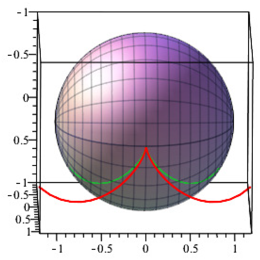
is a framed rectifying curve with a cusp in ${\mathbb{R}}^3$ (Figure 2).

Figure 2. The red curve ${\mathit{\gamma }}_2(s)$ is the framed rectifying curve, and the green curve ${\mathit{g}}_2(s)$ is a curve on $S^2$.

5. Framed Rectifying Curves versus Framed Helices

In this section, we define the framed helices and investigate the relations between framed helices and framed rectifying curves.

Definition 4.

Let $(\mathit{\gamma },{\overline{\mathit{\mu }}}_1,{\overline{\mathit{\mu }}}_2):I\to {\mathbb{R}}^3\times {\Delta }_2$ be a framed curve with $p(s)>0$. We call $\mathit{\gamma }$ a framed helix if there exists a fixed unit vector $\mathit{\zeta }$ satisfying:

$$\begin{array}{c}\hfill ⟨\mathbf{\nu }(s),\mathbf{\zeta }⟩=cos\omega \end{array}$$

for some constant $\omega .$

We now consider the ratio $(q/p)(s)$ of the framed helix.

$$\begin{array}{c}\hfill ⟨\mathbf{\nu }(s),\mathbf{\zeta }⟩=cos\omega .\end{array}$$

(10)

By taking the derivative of (10), as $p(s)>0$ and ${⟨\mathit{\nu }(s),\mathit{\zeta }⟩}^{\prime }=p(s)⟨{\overline{\mathit{\mu }}}_1(s),\mathit{\zeta }⟩$, we have:

$$\begin{array}{c}\hfill ⟨{\overline{\mathbf{\mu }}}_1(s),\mathbf{\zeta }⟩=0.\end{array}$$

(11)

We know that $\mathit{\zeta }$ is in the plane whose basis vectors are $\mathit{\nu }(s)$ and ${\overline{\mathit{\mu }}}_2(s).$ As $⟨\mathit{\nu }(s),\mathit{\zeta }⟩=cos\omega ,$ we have $⟨{\overline{\mathit{\mu }}}_2(s),\mathit{\zeta }⟩=\pm sin\omega .$ By taking the derivative of (11), we get:

$$\begin{array}{c}\hfill -p(s)⟨\mathbf{\nu }(s),\mathbf{\zeta }⟩+q(s)⟨{\overline{\mathbf{\mu }}}_2(s),\mathbf{\zeta }⟩=0,\end{array}$$

then:

$$\begin{array}{c}\hfill \frac{q(s)}{p(s)}=\pm cot\omega .\end{array}$$

(12)

For framed rectifying curves, a simple characterization in terms of the ratio $q(s)/p(s)$ is shown in the following theorem.

Theorem 5.

Let $(\gamma ,{\overline{\mu }}_1,{\overline{\mu }}_2):I\to {\mathbb{R}}^3\times {\Delta }_2$ be a framed curve with $p(s)>0$, then $\gamma (s)$ is a framed rectifying curve if and only if $q(s)/p(s)=c_1\int \alpha (s)ds+c_2$ for some constants $c_1$ and $c_2,$ with $c_1\ne 0.$

Proof. 

The proof is similar to that of Theorem 2 in [4]. If $\mathit{\gamma }(s)$ is a framed rectifying curve, from (2), we have that $q(s)/p(s)=\lambda (s)/\xi (s)=\lambda (s)/\xi$ for some constant $\xi .$ Since ${\lambda }^{\prime }(s)=\alpha (s)$ and $\xi \ne 0,$ then the ratio of $q(s)$ and $p(s)$ satisfies $q(s)/p(s)=c_1\int \alpha (s)ds+c_2$ for some constants $c_1$ and $c_2,$ with $c_1\ne 0.$

Conversely, suppose that $(\mathit{\gamma },{\overline{\mathit{\mu }}}_1,{\overline{\mathit{\mu }}}_2):I\to {\mathbb{R}}^3\times {\Delta }_2$ is a framed curve with $p(s)>0$, and $q(s)/p(s)=c_1\int \alpha (s)ds+c_2$ for some constants $c_1$ and $c_2,$ with $c_1\ne 0.$ If we put $\xi =1/c_1$ and $\lambda (s)=\int \alpha (s)ds+c_2/c_1,$ hence, by invoking the Frenet–Serret formula, we obtain:

$$\begin{array}{c}\hfill \frac{d}{ds}[\mathbf{\gamma }(s)-\lambda (s)\mathbf{\nu }(s)-\xi {\overline{\mathbf{\mu }}}_2(s)]=(\xi q(s)-\lambda (s)p(s)){\overline{\mathbf{\mu }}}_1(s)=0.\end{array}$$

This means that $\mathit{\gamma }(s)$ is congruent to a framed rectifying curve. ☐

Remark 2.

If $\mathit{\gamma }$ is a framed rectifying curve, we have $\lambda (s)p(s)=\xi q(s)$ for some constant $\xi .$ If $\xi =0,$ then $\lambda (s)p(s)=0,$ as $p(s)>0,$ so $\lambda (s)\equiv 0.$ This means that $\mathit{\gamma }(s)$ is a point.

After that, we reveal the relationship between the framed rectifying curves and the framed helices. We have the following theorem:

Theorem 6.

Let $(\mathit{\gamma },{\overline{\mathit{\mu }}}_1,{\overline{\mathit{\mu }}}_2):I\to {\mathbb{R}}^3\times {\Delta }_2$ be a framed curve with $p(s)>0,$ the framed curvature functions satisfying $(q/p)(s)=c_1\int \alpha (s)ds+c_2,$ for some constants $c_1$ and $c_2.$ If $c_1=0,$ we will get framed helices; otherwise, we get framed rectifying curves.

6. Framed Rectifying Curves versus Centrodes

The centrodes play important roles in joint kinematics and mechanics (see [5]). We can define the centrodes of framed curves. For a framed curve $\mathit{\gamma }$ in ${\mathbb{R}}^3,$ the curve defined by the vector $\mathit{d}=q\mathit{\nu }+p{\overline{\mathit{\mu }}}_2$, which is called the centrode of framed curve $\mathit{\gamma }.$

The following results establish some relationships between framed rectifying curves and centrodes.

Theorem 7.

The centrode of a framed curve with nonzero constant framed curvature function $p(s)$ and nonconstant framed curvature function $q(s)$ is a framed rectifying curve. Conversely, the framed rectifying curve in ${\mathbb{R}}^3$ is the centrode of some framed curve with nonconstant framed curvature function $q(s)$ and nonzero constant framed curvature function $p(s)$.

Proof. 

Let $\mathit{\gamma }(s)$ be a framed curve with nonzero constant framed curvature $p(s)$ and nonconstant framed curvature $q(s).$ Consider the centrode of $\mathit{\gamma }(s)$:

$$\begin{array}{c}\hfill \mathbf{d}(s)=q(s)\mathbf{\nu }(s)+p(s){\overline{\mathbf{\mu }}}_2(s).\end{array}$$

$\mathit{d}(s)$ can also be seen as a framed curve. Let the vectors ${\overline{\mathit{\mu }}}_{d,1}(s),{\overline{\mathit{\mu }}}_{d,2}(s),{\mathit{\nu }}_d(s)$ be the adapted frame along $\mathit{d}(s).$ By differentiating the centrode, then we have ${\mathit{d}}^{\prime }(s)=q^{\prime }(s)\mathit{\nu }(s)$, which implies that unit vector ${\mathit{\nu }}_d(s)$ and unit vector $\mathit{\nu }(s)$ at the corresponding points are parallel. Then, the first equality in Frenet–Serret formula implies that ${\overline{\mathit{\mu }}}_{d,1}(s)$ and ${\overline{\mathit{\mu }}}_1(s)$ at the corresponding points are also parallel. Hence, ${\overline{\mathit{\mu }}}_{d,2}(s)$ and ${\overline{\mathit{\mu }}}_2(s)$ are parallel, as well. Therefore, by definition, the centrode $\mathit{d}(s)$ is a framed rectifying curve.

Conversely, let $\mathit{\gamma }(s)$ be a framed rectifying curve in ${\mathbb{R}}^3.$ From Theorem 3, we have:

$$\begin{array}{c}\hfill {\lambda }^{\prime }(s)=\alpha (s),\lambda (s)p(s)=cq(s)\end{array}$$

(13)

for some constant $c.$

Let $f(s)=\frac{1}{c}{\int }_{s_0}^{s}p(u)du.$ There exists a framed curve $\mathit{\beta }(t)$ whose framed curvature satisfies $p_{\beta }(t)=c$ and $q_{\beta }(t)=\lambda (t).$

Let us consider the centrode of $\beta$, which is given by ${\mathit{d}}_{\beta }(t)=\lambda (t){\mathit{\nu }}_{\beta }(t)+c{\overline{\mathit{\mu }}}_{\beta ,2}(t)$, and its reparametrization $\mathit{\chi }(s)={\mathit{d}}_{\beta }(f(s)).$ Then:

$$\begin{array}{c}\hfill \mathbf{\chi }(s)=\lambda (f(s)){\mathbf{\nu }}_{\beta }(f(s))+c{\overline{\mathbf{\mu }}}_{\beta ,2}(f(s)).\end{array}$$

This means that ${\mathit{\chi }}^{\prime }(s)=\alpha (s){\mathit{\nu }}_{\beta }(f(s));$ thus, ${\mathit{\nu }}_{\chi }(s)={\mathit{\nu }}_{\beta }(f(s)).$ Differentiating twice, the framed curvature functions of $\mathit{\chi }$ are given by ${\alpha }_{\chi }(s)=\alpha (s),$$p_{\chi }(s)=p_{\beta }(s)f^{\prime }(s)=p(s)$ and $q_{\chi }(s)=q_{\beta }(s)f^{\prime }(s)=q(s).$

Therefore, the framed curves $\mathit{\gamma }(s)$ and $\mathit{\chi }(s)$ have the same framed curvature functions. From the existence theorem and the uniqueness theorem, it follows that $\mathit{\chi }$ is congruent to $\mathit{\gamma }.$ Consequently, the framed rectifying curve $\mathit{\gamma }$ is the centrode of a framed curve with nonconstant framed curvature $q(s)$ and nonzero constant framed curvature p. ☐

The framed curve in Theorem 7 can be replaced by a framed curve with nonzero constant framed curvature q and nonconstant framed curvature $p(s).$ In fact, we also have the following theorem:

Theorem 8.

The centrode of a framed curve with nonzero constant framed curvature function $q(s)$ and nonconstant framed curvature function $p(s)$ is a framed rectifying curve. Conversely, one framed rectifying curve in ${\mathbb{R}}^3$ is the centrode of some framed curve with nonconstant framed curvature function $p(s)$ and nonzero constant framed curvature function $q(s)$.

The proof can be given in as similar way as Theorem 7.

Remark 3.

The centrode of a framed curve with nonzero constant framed curvature function $p(s)$ and nonzero constant framed curvature function $q(s)$ is a point.

7. Contact between Framed Rectifying Curves

In this section, the contact between framed rectifying curves is considered. We now introduce the notion of circular rectifying curves as follows.

Definition 5.

Let $\mathit{\gamma }(s)$ be a framed rectifying curve and:

$$\begin{array}{c}\hfill \mathbf{\gamma }(s)=\rho ({tan}^2(\int |{\mathit{g}}^{\prime }{(s)|ds+C)+1)}^{\frac{1}{2}}\mathit{g}(s),\end{array}$$

where ρ is a positive number and C is a constant. We call $\mathit{\gamma }$ a circular rectifying curve if $\mathit{g}(s)$ is a circle on $S^2$.

Let $(\mathit{\gamma },{\mathit{\mu }}_1,{\mathit{\mu }}_2):I\to S^2\times {\Delta }_2$ be a framed spherical curve. We choose ${\mathit{\mu }}_1=\mathit{\gamma }$, then $\mathit{\nu }=\mathit{\gamma }\times {\mathit{\mu }}_2$ and ${\mathit{\gamma }}^{\prime }(s)=\alpha (s)\mathit{\nu }(s)$. We show that the spherical Frenet–Serret formula of $\mathit{\gamma }$ is as follows:

$$\left\{\begin{array}{c}{\mathit{\gamma }}^{\prime }(s)=\alpha (s)\mathit{\nu }(s)\hfill \\ {\mathit{\mu }}_2^{\prime }(s)=l(s)\mathit{\nu }(s)\hfill \\ {\mathit{\nu }}^{\prime }(s)=-\alpha (s)\mathit{\gamma }(s)-l(s){\mathit{\mu }}_2(s),\hfill \end{array}\right.$$

where $⟨{\mathit{\mu }}_2^{\prime }(s),\mathit{\nu }(s)⟩=l(s)$. By the curvature functions $\alpha (s)$ and $l(s)$, we show the following proposition for framed spherical curves:

Proposition 2.

Let $(\mathit{\gamma },\mathit{\gamma },{\mathit{\mu }}_2):I\to S^2\times {\Delta }_2$ be a framed spherical curve, then $\mathit{\gamma }$ is a circle if and only if $\alpha (s)\ne 0$ and $l(s)/\alpha (s)=constant$.

Proof 

If $\alpha (s)\ne 0$ and $(l/\alpha )(s)=k$, where k is a constant, then we consider a normal vector field $\mathit{N}(s)=\frac{k^2}{k^2+1}\mathit{\gamma }(s)-\frac{k}{k^2+1}{\mathit{\mu }}_2(s)$. By taking the derivative of $\mathit{N}(s)$, we have ${\mathit{N}}^{\prime }(s)=\frac{k^2}{k^2+1}(\alpha (s)\mathit{\nu }(s)-\alpha (s)\mathit{\nu }(s))=\mathbf{0}$. This means that $\mathit{N}(s)$ is a constant vector. Moreover, we have:

$$\begin{array}{c}\hfill ⟨\mathbf{N}(s),\mathbf{\gamma }(s)-\mathbf{N}(s)⟩=⟨\frac{k^2}{k^2+1}\mathbf{\gamma }(s)-\frac{k}{k^2+1}{\mathbf{\mu }}_2(s),\frac{1}{k^2+1}\mathbf{\gamma }(s)+\frac{k}{k^2+1}{\mathbf{\mu }}_2(s)⟩=0.\end{array}$$

This means that $\mathit{\gamma }$ is the intersection of a plane and $S^2$, so $\mathit{\gamma }$ is a circle.

Let $\mathit{\gamma }$ be a circle on $S^2$. Obviously, $\mathit{\gamma }$ is a plane curve and $\alpha (s)\ne 0$, so that $⟨{\mathit{\gamma }}^{\prime }(s),{\mathit{\gamma }}^{″}(s)\times {\mathit{\gamma }}^{‴}(s)⟩=0.$ Then, we can calculate that $⟨{\mathit{\gamma }}^{\prime }(s),{\mathit{\gamma }}^{″}(s)\times {\mathit{\gamma }}^{‴}(s)⟩={\alpha }^4(s)l^{\prime }(s)-{\alpha }^3(s){\alpha }^{\prime }(s)l(s)$. Since $\alpha (s)\ne 0$, we have $\alpha (s)l^{\prime }(s)-{\alpha }^{\prime }(s)l(s)=0$. This is equivalent to ${(l/\alpha )}^{\prime }(s)=0$. Thus, $l(s)/\alpha (s)=constant$. $\square$

As a corollary of Proposition 2, we have the following result:

Corollary 1.

Let $(\mathit{\gamma },\mathit{\gamma },{\mathit{\mu }}_2):I\to S^2\times {\Delta }_2$ be a framed spherical curve, then $\mathit{\gamma }$ is a great circle on $S^2$ if and only if $\alpha (s)\ne 0$ and $l(s)=0$.

Now, we review the notions of contact between framed curves [14]. Let $(\mathit{\gamma },{\mathit{\mu }}_1,{\mathit{\mu }}_2):I\to {\mathbb{R}}^3\times {\Delta }_2$; $s\to (\mathit{\gamma }(s),{\mathit{\mu }}_1(s),{\mathit{\mu }}_2(s))$ and $(\tilde{\mathit{\gamma }},{\tilde{\mathit{\mu }}}_1,{\tilde{\mathit{\mu }}}_2):\tilde{I}\to {\mathbb{R}}^3\times {\Delta }_2$; $u\to (\tilde{\mathit{\gamma }}(u),{\tilde{\mathit{\mu }}}_1(u),{\tilde{\mathit{\mu }}}_2(u))$ be framed curves. We say that $(\mathit{\gamma },{\mathit{\mu }}_1,{\mathit{\mu }}_2)$ and $(\tilde{\mathit{\gamma }},{\tilde{\mathit{\mu }}}_1,{\tilde{\mathit{\mu }}}_2)$ have $k^{\mathrm{th}}$ order contact at $s=s_0$, $u=u_0$ if:

$$\begin{array}{c}(\mathbf{\gamma },{\mathbf{\mu }}_1,{\mathbf{\mu }}_2)(s_0)=(\tilde{\mathbf{\gamma }},{\tilde{\mathbf{\mu }}}_1,{\tilde{\mathbf{\mu }}}_2)(u_0),\frac{d}{ds}(\mathbf{\gamma },{\mathbf{\mu }}_1,{\mathbf{\mu }}_2)(s_0)=\frac{d}{du}(\tilde{\mathbf{\gamma }},{\tilde{\mathbf{\mu }}}_1,{\tilde{\mathbf{\mu }}}_2)(u_0),\dots ,\hfill \\ \frac{d^{k-1}}{d{s}^{k-1}}(\mathbf{\gamma },{\mathbf{\mu }}_1,{\mathbf{\mu }}_2)(s_0)=\frac{d^{k-1}}{d{u}^{k-1}}(\tilde{\mathbf{\gamma }},{\tilde{\mathbf{\mu }}}_1,{\tilde{\mathbf{\mu }}}_2)(u_0),\frac{d^k}{d{s}^k}(\mathbf{\gamma },{\mathbf{\mu }}_1,{\mathbf{\mu }}_2)(s_0)\ne \frac{d^k}{d{u}^k}(\tilde{\mathbf{\gamma }},{\tilde{\mathbf{\mu }}}_1,{\tilde{\mathbf{\mu }}}_2)(u_0).\hfill \end{array}$$

In addition, we say that $(\mathit{\gamma },{\mathit{\mu }}_1,{\mathit{\mu }}_2)$ and $(\tilde{\mathit{\gamma }},{\tilde{\mathit{\mu }}}_1,{\tilde{\mathit{\mu }}}_2)$ have at least $k^{\mathrm{th}}$ order contact at $s=s_0$, $u=u_0$ if:

$$\begin{array}{c}(\mathbf{\gamma },{\mathbf{\mu }}_1,{\mathbf{\mu }}_2)(s_0)=(\tilde{\mathbf{\gamma }},{\tilde{\mathbf{\mu }}}_1,{\tilde{\mathbf{\mu }}}_2)(u_0),\frac{d}{ds}(\mathbf{\gamma },{\mathbf{\mu }}_1,{\mathbf{\mu }}_2)(s_0)=\frac{d}{du}(\tilde{\mathbf{\gamma }},{\tilde{\mathbf{\mu }}}_1,{\tilde{\mathbf{\mu }}}_2)(u_0),\dots ,\hfill \\ \frac{d^{k-1}}{d{s}^{k-1}}(\mathbf{\gamma },{\mathbf{\mu }}_1,{\mathbf{\mu }}_2)(s_0)=\frac{d^{k-1}}{d{u}^{k-1}}(\tilde{\mathbf{\gamma }},{\tilde{\mathbf{\mu }}}_1,{\tilde{\mathbf{\mu }}}_2)(u_0).\hfill \end{array}$$

We generally say that $(\mathit{\gamma },{\mathit{\mu }}_1,{\mathit{\mu }}_2)$ and $(\tilde{\mathit{\gamma }},{\tilde{\mathit{\mu }}}_1,{\tilde{\mathit{\mu }}}_2)$ have at least first order contact at any point $s=s_0$, $u=u_0$, up to congruence as framed curves. As a conclusion of Theorem 3.7 in [14], we show the following proposition:

Proposition 3.

Let $(\mathit{\gamma },\mathit{\gamma },{\mathit{\mu }}_2):I\to S^2\times {\Delta }_2$, $s\to (\mathit{\gamma }(s),\mathit{\gamma }(s),{\mathit{\mu }}_2(s))$ and $(\tilde{\mathit{\gamma }},\tilde{\mathit{\gamma }},{\tilde{\mathit{\mu }}}_2):\tilde{I}\to S^2\times {\Delta }_2$, $u\to (\tilde{\mathit{\gamma }}(u),\tilde{\mathit{\gamma }}(u),{\tilde{\mathit{\mu }}}_2(u))$ be framed spherical curves. If $(\mathit{\gamma },\mathit{\gamma },{\mathit{\mu }}_2)$ and $(\tilde{\mathit{\gamma }},\tilde{\mathit{\gamma }},{\tilde{\mathit{\mu }}}_2)$ have at least ${(k+1)}^{\mathrm{th}}$ order contact at $s=s_0$, $u=u_0$, we have:

$$\begin{array}{cc}\hfill & \alpha (s_0)=\tilde{\alpha }(u_0),\frac{d}{ds}\alpha (s_0)=\frac{d}{du}\tilde{\alpha }(u_0),\dots ,\frac{d^{k-1}}{d{s}^{k-1}}\alpha (s_0)=\frac{d^{k-1}}{d{u}^{k-1}}\tilde{\alpha }(u_0),\hfill \end{array}$$

(14)

$$\begin{array}{cc}\hfill & l(s_0)=\tilde{l}(u_0),\frac{d}{ds}l(s_0)=\frac{d}{du}\tilde{l}(u_0),\dots ,\frac{d^{k-1}}{d{s}^{k-1}}l(s_0)=\frac{d^{k-1}}{d{u}^{k-1}}\tilde{l}(u_0).\hfill \end{array}$$

(15)

Conversely, if the conditions (14) and (15) hold, then $(\mathit{\gamma },\mathit{\gamma },{\mathit{\mu }}_2)$ and $(\tilde{\mathit{\gamma }},\tilde{\mathit{\gamma }},{\tilde{\mathit{\mu }}}_2)$ have at least ${(k+1)}^{\mathrm{th}}$ order contact at $s=s_0$, $u=u_0$, up to congruence as framed spherical curves.

Now, we consider the contact between circles and framed spherical curves. We have a corollary of Propositions 2 and 3 as follows:

Corollary 2.

Let $(\mathit{\gamma },\mathit{\gamma },{\mathit{\mu }}_2):I\to S^2\times {\Delta }_2$ be a framed spherical curve. $\mathit{\gamma }$ and a circle have at least ${(k+1)}^{\mathrm{th}}$ order contact at $s=s_0$ if and only if there exists a constant σ such that:

$$\begin{array}{c}\hfill l(s_0)=\sigma \alpha (s_0),\frac{d}{ds}l(s_0)=\sigma \frac{d}{ds}\alpha (s_0),\dots ,\frac{d^{k-1}}{d{s}^{k-1}}l(s_0)=\sigma \frac{d^{k-1}}{d{s}^{k-1}}\alpha (s_0).\end{array}$$

For the construction of the framed rectifying curve in Theorem 4, we fix positive number $\rho$ and constant C. Let ${\mathit{g}}_i:I\to S^2$$(i=1,2)$ be framed spherical curves. We know ${\mathit{\gamma }}_1$, ${\mathit{\gamma }}_2$ have $k^{\mathrm{th}}$ order contact at $s_0$ if and only if ${\mathit{g}}_1$, ${\mathit{g}}_2$ have $k^{\mathrm{th}}$ order contact at $s_0$. By Corollary 2, we have the following theorem, which can describe the contact between framed rectifying curves and circular rectifying curves.

Theorem 9.

Let $\mathit{\gamma }$ be a framed rectifying curve and $\alpha (s)$ and $l(s)$ be curvature functions of the corresponding framed spherical curve. Then, $\mathit{\gamma }$ and a circular rectifying curve have at least $k^{\mathrm{th}}$ order $(k\ge 2)$ contact at $s_0$ if and only if there exists a constant σ such that:

$$\begin{array}{c}\hfill l(s_0)=\sigma \alpha (s_0),\frac{d}{ds}l(s_0)=\sigma \frac{d}{ds}\alpha (s_0),\dots ,\frac{d^{k-2}}{d{s}^{k-2}}l(s_0)=\sigma \frac{d^{k-2}}{d{s}^{k-2}}\alpha (s_0).\end{array}$$

References

- Mikula, K.; Sevcovic, D. Evolution of curves on a surface driven by the geodesic curvature and external force. Appl. Anal. 2006, 85, 345–362. [Google Scholar] [CrossRef] [Green Version]
- Izumiya, S.; Takeuchi, N. Generic properties of helices and Bertrand curves. J. Geom. 2002, 74, 97–109. [Google Scholar] [CrossRef]
- Liu, Y.; Ru, M. Degeneracy of holomorphic curves in surfaces. Sci. China Ser. A 2005, 48, 156–167. [Google Scholar] [CrossRef]
- Chen, B.Y. When does the position vector of a space curve always lie in its rectifying plane? Am. Math. Mon. 2003, 110, 147–152. [Google Scholar] [CrossRef]
- Chen, B.Y.; Dillen, F. Rectifying curves as centrodes and extremal curves. Bull. Inst. Math. Acad. Sin. 2005, 33, 77–90. [Google Scholar]
- Yeh, H.; Abrams, J.I. Principles of Mechanics of Solids and Fluids; McGraw-Hill: New York, NY, USA, 1960; Volume 1. [Google Scholar]
- Ogston, N.; King, G.; Gertzbein, S.; Tile, M.; Kapasouri, A.; Rubenstein, J. Centrode patterns in the lumbar spine-base-line studies in normal subjects. Spine 1986, 11, 591–595. [Google Scholar] [CrossRef] [PubMed]
- Weiler, P.J.; Bogoch, R.E. Kinematics of the distal radioulnar joint in rheumatoid-arthritis-an in-vivo study using centrode analysis. J. Hand Surg. 1995, 20, 937–943. [Google Scholar] [CrossRef]
- Gertzbein, S.; Seligman, J.; Holtby, R.; Chan, K.; Ogston, N.; Kapasouri, A.; Tile, M.; Cruickshank, B. Centrode patterns and segmental instability in degenerative disk disease. Spine 1985, 10, 257–261. [Google Scholar] [CrossRef] [PubMed]
- Πarslan, K.; Nesovic, E. On rectifying curves as centrodes and extremal curves in the Minkowski 3-space. Novi Sad J. Math. 2007, 37, 53–64. [Google Scholar]
- Πarslan, K.; Nesovic, E. Some characterizations of null, pseudo null and partially null rectifying curves in Minkowski space-time. Taiwan. J. Math. 2008, 12, 1035–1044. [Google Scholar]
- Πarslan, K.; Nesovic, E. Some characterizations of rectifying curves in the Euclidean space E4. Turk. J. Math. 2008, 32, 21–30. [Google Scholar]
- Grbovic, M.; Nesovic, E. Some relations between rectifying and normal curves in Minkowski 3-space. Math. Commun. 2012, 17, 655–664. [Google Scholar]
- Honda, S.; Takahashi, M. Framed curves in the Euclidean space. Adv. Geom. 2016, 16, 265–276. [Google Scholar] [CrossRef]
- Chen, L.; Takahashi, M. Dualities and evolutes of fronts in hyperbolic and de Sitter space. J. Math. Anal. Appl. 2016, 437, 133–159. [Google Scholar] [CrossRef] [Green Version]
- Bishop, R.L. There is more than one way to frame a curve. Am. Math. Mon. 1975, 82, 246–251. [Google Scholar] [CrossRef]
Figure 1.
The red curve is the regular rectifying curve, and the green curve is a curve on .
Figure 2.
The red curve is the framed rectifying curve, and the green curve is a curve on .
© 2019 by the authors. Licensee MDPI, Basel, Switzerland. This article is an open access article distributed under the terms and conditions of the Creative Commons Attribution (CC BY) license (http://creativecommons.org/licenses/by/4.0/).
Share and Cite
MDPI and ACS Style
Wang, Y.; Pei, D.; Gao, R. Generic Properties of Framed Rectifying Curves. Mathematics 2019, 7, 37. https://doi.org/10.3390/math7010037
AMA Style
Wang Y, Pei D, Gao R. Generic Properties of Framed Rectifying Curves. Mathematics. 2019; 7(1):37. https://doi.org/10.3390/math7010037
Chicago/Turabian StyleWang, Yongqiao, Donghe Pei, and Ruimei Gao. 2019. "Generic Properties of Framed Rectifying Curves" Mathematics 7, no. 1: 37. https://doi.org/10.3390/math7010037
Note that from the first issue of 2016, this journal uses article numbers instead of page numbers. See further details here.