Distance and Adjacency Energies of Multi-Level Wheel Networks

Abstract

Energies of molecular graphs have various applications in chemistry, polymerization, computer networking and pharmacy. In this paper, we give general closed forms of distance and adjacency energies of generalized wheel networks $W_{n,m}$. Consequently, we give these results for classical wheel graphs. We also give pictorial dependencies of energies on the involved parameters $m\ge 3$ and $n$.

1. Introduction

Energy is referred to as the sum of absolute values of any operator. In quantum chemistry, the solutions of the Schrodinger equation is approximately reduced to the evaluation of eigenvalues and corresponding eigenvectors of the Hamiltonian operator. Often, Hamiltonian operators are approximately expressed as

$$H=\alpha I+\beta A\left(G\right),$$

(1)

where $\alpha$ and $\beta$ are the empirical constants of Huckel molecular orbital theory and $A\left(G\right)$ is the adjacency matrix of the Huckel graph constructed for the $\pi$-electron network of conjugated hydro-carbons [1]. In this way, characteristic polynomials entered the arena of chemical graph theory. It has also attracted keen interest even from pure mathematicians due to the interesting problems that originate from the mathematical structures and their symmetries involved. The ordinary energy of the graph is defined as the sum of the absolute values of the eigenvalues of its adjacency matrix. This graph invariant is very closely connected to a chemical quantity known as the total $\pi$-electron energy of conjugated hydro-carbon molecules. In recent times, analogous energies are being considered, based on eigenvalues of a variety of other graph matrices associated to the graph [1,2,3,4]. In [5], authors computed incidence energy of a graph. In [6], authors computed general forms of energies of non-regular graphs.

Gutman introduced this idea of the energy of a graph in 1978 in the context of Mathematics [4]; however, inspiration for his definition seems to emerge from the popular Huckel molecular orbital theory. Huckel’s technique enabled scientific experts to predict energies related to p-electron orbitals for a unique class of particles. The basic idea behind this is the Hamiltonian operator, which is a basic linear combination of certain orbitals [7,8]. It is somewhat less known than the one Heilbronner et al. developed, a model resulting in a fact that the roots of the characteristic polynomial of the line graph of the molecular graph are in a linear manner related to the s-electron energy levels of the corresponding saturated hydrocarbon [7,8], where these molecular graphs have vertices of both carbon and hydrogen atoms. Its popularity among mathematical chemists came from the fact that the Hamiltonian matrix of the Huckel molecular orbital theory is a simple linear function of the adjacency matrix of the corresponding molecular graph G. Thus, each $\pi$-electron energy level is a linear function of the corresponding zero of the characteristic polynomial of G [9]. In addition, under certain sensible presumptions about the particle, its “aggregate $\pi$ electron energy” can be composed as the sum of the total eigenvalues of this graph.

Since the definition of energy for a graph in [4] is rather strange, not many mathematicians appear to be pulled by the definition. However, with the passage of time, the idea became powerful and in the previous decade enthusiasm for graph energy has expanded resulting in numerous different forms [3]. In 2006, Gutman and Zhou defined the Laplacian energy of a graph [10]. The authors of [11,12] discussed distance energy of a graph based on the idea of distance matrix associated with the graph. Nikiforov et al. computed some energies of non-regular graphs [13]. In [14], the authors discussed signless Laplacian energies of some finite graphs. In [15], the author discussed graph theoretical analyses in analyzing the changes in interactions between solvent and solute. In [16,17], the authors computed some asymptotic Laplacian and incidence energies of lattice.

Let G be a graph having vertex set $V\left(G\right)$ and edge set $E\left(G\right)$ denoted by $G=(V,E)$. A Graph $G=(V,E)$ is said to be connected if there is a connection between any pair of vertices in G. The number of vertices in a graph represents its order, the number of edges represents its size, and the number of edges connected to a single vertex represents the degree of that vertex denoted as $d_u$. The distance matrix associated to a graph is defined as the square matrix $D=\left[d_{ab}\right]$ where $d_{ab}$ consists of all graph distances from vertex $v_a$ to vertex $v_b$. An $n\times n$ matrix M for a graph having order n, called an adjacency matrix, can be associated to the graph as,

$$\left[M_{ab}\right]=\left\{\begin{array}{c}1p_1\mapsto p_2\hfill \\ 0\mathrm{otherwise}\hfill \end{array}\right\}$$

The roots of a characteristics polynomial are the eigenvalues of a matrix associated to a graph. In most cases, the associated matrices are real and symmetric so eigenvalues are necessarily real-valued numbers. The collection of all eigenvalues of graph G forms the spectrum of $G$. Spectral properties of graphs have been widely studied. If G is not connected, then the energy of a graph is the sum of energies of its connected components. If a graph is connected, then its distance and adjacency energies are defined as the sum of the absolute values of associated eigenvalues. Energy of some non-regular graphs and Laplacian energy of a simple graph are discussed in [14,18].

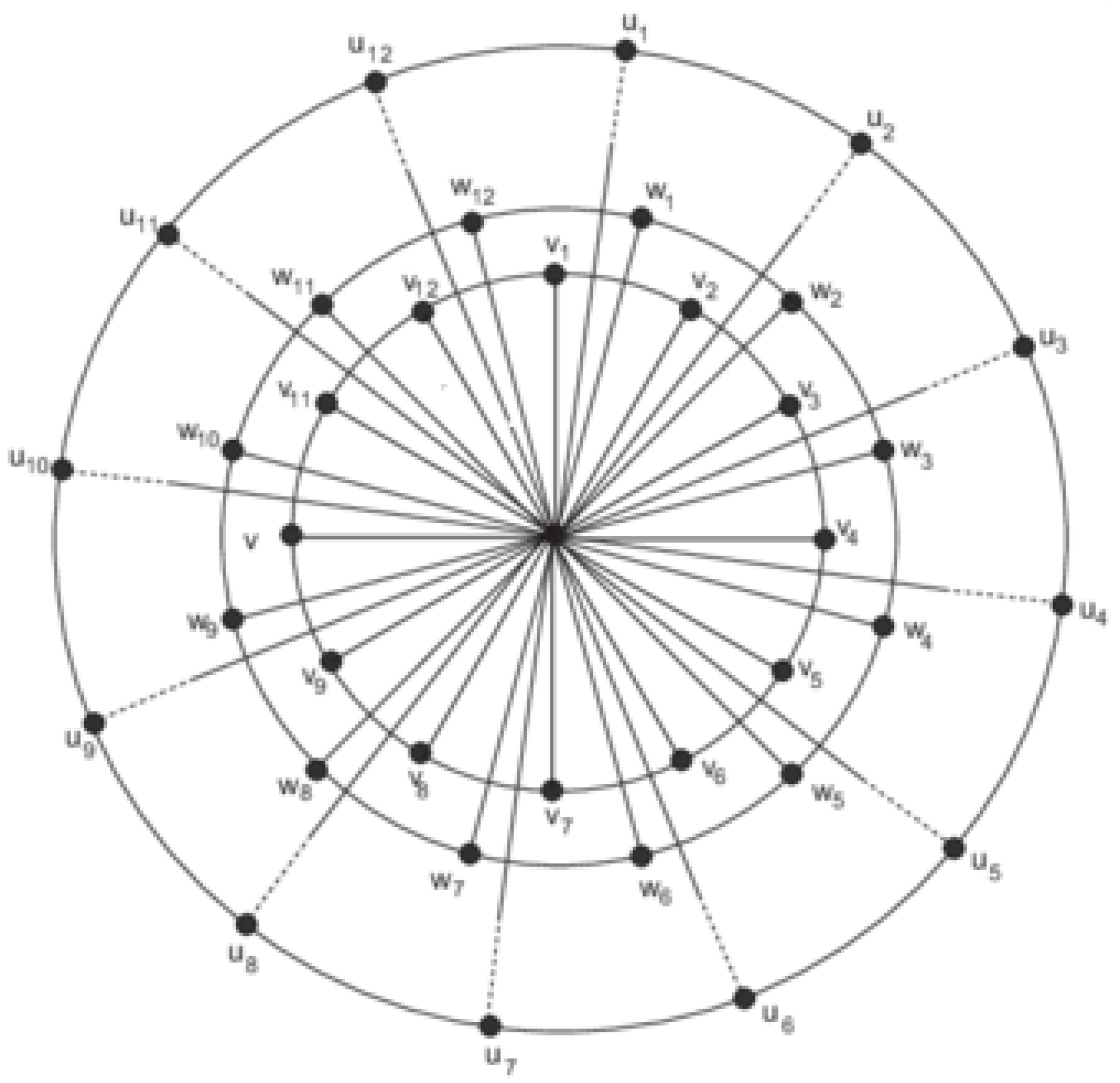
In the current article, we want to find closed expressions for distance and adjacency energies of generalized wheel graphs, also known as m-level wheel, $W_{n,m}.$ An m-wheel graph $W_{n,m}$ is a graph obtained from m copies of cycles $C_n$ and one copy of vertex $v$, such that all vertices of every copy of $C_n$ are adjacent to v. Thus, $W_{n,m}$ has $nm+1$ vertices, i.e., the center and n-rim vertices, and has diameter 2. Figure 1 is an example of m-wheel graph $W_{12,m}$.

Vertices that lay on the same cycle $C_n$ and adjacent to central vertex are termed as rim vertices. This graph can be considered as generalization of classical wheel graph $W_n$. Figure 2 is another instance of m-wheel graph, $W_{3,4}$.

This m-wheel network is an extension of the classical wheel graph $W_{1,n}$. Figure 3 is an example of wheel graph $W_6$.

The wheel graph has been used in different areas such as the wireless sensor networks and the vulnerability of networks [19]. The wheel graph has many good properties. From the standpoint of the hub vertex, all elements, including vertices and edges, are in its one-hop neighborhood, which indicates that the wheel structure is fully included in the neighborhood graph of the hub vertex. Wheel and related graphs are extensively studied recently. In [20], the authors computed partition dimension and connected partition dimension of wheel graphs and showed that, for $n\ge 4$, ${\left[\left(2n\right)\right]}^{\frac{1}{3}}\le pd\left(G\right)\le 2\left[n^{\frac{1}{2}}\right]+1$. In [21], the authors gave an algorithm to compute average lower two-domination number and also computed this number for some wheel related graphs. In [22], authors computed the metric dimension of generalised wheel. In [23], Zafar et al. generalized the above results to multi-level wheel and obtained that for every $n\ge 4$, ${\left[\left(2nm\right)\right]}^{\frac{1}{3}}\le pd\left(W_{n,m}\right)\le 2\left[n{m}^{\frac{1}{2}}\right]+1$.

2. Main Results

In this section, we give some results on distance and adjacency energies of wheel related graphs $W_{n,m}$.

Theorem 1.

The distance energy of the wheel graph $W_{n,m}$ is given by

$$E_D\left(W_{n,m}\right)=2(mn-2+\sqrt{m^2{n}^2-3mn+4}),$$

(2)

where $m\ge 3$ and $n\ge 1$.

Proof. 

Let A be adjacency matrix of cycle graph $C_m$ given by

$$A=\left(\begin{array}{ccccccccc}0& 1& 0& 0& .& .& .& 0& 1\\ 1& 0& 1& 0& .& .& .& 0& 0\\ 0& 1& 0& 1& .& .& .& 0& 0\\ 0& 0& 1& 0& .& .& .& 0& 0\\ .& .& .& .& .& .& .& .& .\\ .& .& .& .& .& .& .& .& .\\ .& .& .& .& .& .& .& .& .\\ 0& 0& 0& 0& .& .& .& 0& 1\\ 1& 0& 0& 0& .& .& .& 1& 0\end{array}\right)$$

where $a_{ij}=1$ for $|i-j|=1$ or $m-1$ and $a_{ij}=0$ otherwise.

Generally, the m-cycle has adjacency spectrum

$$Spec\left(C_m\right)=2cos(\frac{2\pi j}{m})wherej=0,1,2,\dots n-1.$$

The distance matrix of wheel graph $W_{n,m}$ obtained by joining of m-vertex cycle $C_m$ and $K_n$ can be given as,

$$C_{m\times m}=\left(\begin{array}{ccccccc}0& J_{1\times m}& J_{1\times m}& .& .& .& J_{1\times m}\\ J_{m\times 1}& {[A+2\overline{A}]}_{m\times m}& T_{m\times m}& .& .& .& T_{m\times m}\\ J_{m\times 1}& T_{m\times m}& {[A+2\overline{A}]}_{m\times m}& .& .& .& T_{m\times m}\\ .& .& .& .& .& .& .\\ .& .& .& .& .& .& .\\ .& .& .& .& .& .& .\\ J_{m\times 1}& T_{m\times m}& T_{m\times m}& .& .& .& T_{m\times m}\\ J_{m\times 1}& T_{m\times m}& T_{m\times m}& .& .& .& {[A+2\overline{A}]}_{m\times m}\end{array}\right)$$

where

$$J_{1\times m}=\left(\begin{array}{cccccc}1& 1& .& .& .& 1\end{array}\right),$$

$$T_{m\times m}=\left(\begin{array}{cccccc}2& 2& .& .& .& 2\\ 2& 2& .& .& .& 2\\ .& .& .& .& .& .\\ .& .& .& .& .& .\\ .& .& .& .& .& .\\ 2& 2& .& .& .& 2\end{array}\right),$$

and

$$A+2\overline{A}=\left(\begin{array}{ccccccccc}0& 1& 2& 2& .& .& .& 1& 1\\ 1& 0& 1& 2& .& .& .& 2& 1\\ 2& 1& 0& 1& .& .& .& 2& 1\\ .& .& .& .& .& .& .& .& .\\ .& .& .& .& .& .& .& .& .\\ .& .& .& .& .& .& .& .& .\\ 1& 2& 2& 2& .& .& .& 0& 1\\ 1& 1& 1& 1& .& .& .& 1& 0\end{array}\right).$$

We get the distance spectrum of $W_{n,m}$ by using binomial series and adjacency spectrum of cycle graph. Thus, we get,

$$spe{c}_D\left(W_{n,m}\right)=\left(\begin{array}{ccc}mn-2\pm \sqrt{m^2{n}^2-3mn+4}& -4& -({\lambda }_i+2)\\ 1& n-1& n\end{array}\right)fori=2,3,...,m,$$

where ${\lambda }_i$ are the eigenvalues of the adjacency matrix of cycle graph.

Since ${\lambda }_i>0$ for all $i=2,3,\dots ,p$, by using the definition and summing up the eigenvalues, we arrive at the desired result of distance energy, which is $E_D\left(W_{n,m}\right)=2(mn-2+\sqrt{m^2{n}^2-3mn+4})$. □

Theorem 2.

The adjacency energy of the wheel graph $W_{n,m}$ is given by

$$E_A\left(W_{n,m}\right)=4n-2+2\sqrt{nm+1}$$

(3)

where m is even.

Proof. 

Let A be adjacency matrix of cycle graph $C_m$.

$$A=\left(\begin{array}{ccccccccc}0& 1& 0& 0& .& .& .& 0& 1\\ 1& 0& 1& 0& .& .& .& 0& 0\\ 0& 1& 0& 1& .& .& .& 0& 0\\ 0& 0& 1& 0& .& .& .& 0& 0\\ .& .& .& .& .& .& .& .& .\\ .& .& .& .& .& .& .& .& .\\ .& .& .& .& .& .& .& .& .\\ 0& 0& 0& 0& .& .& .& 0& 1\\ 1& 0& 0& 0& .& .& .& 1& 0\end{array}\right)$$

where $a_{ij}=1$ if $|i-j|=1$ or $m-1$ and $a_{ij}=0$ otherwise.

Generally, the m cycles has adjacency spectrum.

$$Spec\left(C_m\right)=2cos(\frac{2\pi j}{m})wherej=0,1,2,\dots n-1.$$

Then, the adjacency matrix of wheel graph $W_{n,m}$ obtained by joining of m-vertex cycle $C_m$ and $K_n$ can be given as,

$$T_{m\times m}=\left(\begin{array}{ccccccc}0& J_{1\times m}& J_{1\times m}& .& .& .& J_{1\times m}\\ J_{m\times 1}& {\left[B\right]}_{m\times m}& {\left[0\right]}_{m\times m}& .& .& .& {\left[0\right]}_{m\times m}\\ J_{m\times 1}& {\left[0\right]}_{m\times m}& {\left[B\right]}_{m\times m}& .& .& .& {\left[0\right]}_{m\times m}\\ .& .& .& .& .& .& .\\ .& .& .& .& .& .& .\\ .& .& .& .& .& .& .\\ J_{m\times 1}& {\left[0\right]}_{m\times m}& {\left[0\right]}_{m\times m}& .& .& .& {\left[0\right]}_{m\times m}\\ J_{m\times 1}& {\left[0\right]}_{m\times m}& {\left[0\right]}_{m\times m}& .& .& .& {\left[B\right]}_{m\times m}\end{array}\right),$$

where

$$J_{1\times m}=\left(\begin{array}{cccccc}1& 1& .& .& .& 1\end{array}\right),$$

and

$$B_{m\times m}=\left(\begin{array}{ccccccccc}0& 1& 0& 0& .& .& .& 0& 1\\ 1& 0& 1& 0& .& .& .& 0& 0\\ 0& 1& 0& 1& .& .& .& 0& 0\\ .& .& .& .& .& .& .& .& .\\ .& .& .& .& .& .& .& .& .\\ .& .& .& .& .& .& .& .& .\\ 0& 0& 0& 0& .& .& .& 0& 1\\ 1& 0& 0& 0& .& .& .& 1& 0\end{array}\right).$$

We get the following adjacency spectrum of $W_{n,m}$ by using binomial series and adjacency spectrum of a cycle graph.

$$spe{c}_A\left(W_{n,m}\right)=\left(\begin{array}{cccc}-2& 2& 1\pm \sqrt{mn+1}& {\lambda }_i\\ n& n-1& 1& n\end{array}\right),fori=3,4,\dots ,m,$$

where ${\lambda }_i$ are the eigenvalues of the adjacency matrix of cycle graph.

As ${\lambda }_i>0$ for all $i=2,3,\dots ,p$, by using the definition and summing up the eigenvalues, we arrive at the desired result of adjacency energy, $E_A\left(W_{n,m}\right)=4n-2+2\sqrt{nm+1}$. □

Theorem 3.

Distance energy of wheel graph $W_{3,m}$ is

$$E_D\left(W_{3,m}\right)=2(3m-2+\sqrt{9m^2-9m+4})$$

(4)

Proof. 

As a classical wheel is a special case of generalized wheels for $n=3$, the proof follows immediately from the first result. □

Theorem 4.

Adjacency energy of wheel graph $W_{3,m}$ is

$$E_A\left(W_{3,m}\right)=10+2\sqrt{3m+1}$$

(5)

Proof. 

As a classical wheel is a special case of generalized wheels for $n=3$, the proof follows immediately from the second result. □

Conclusion and Analysis

In the current article, we compute general forms of distance and adjacency energies of multi-level wheels, which are the extension of classical wheel graph. In the attached figure, dependencies of distance energies on the parameters m and n are given. Figure 4 represents the trends of distance energies with change in m and n. The first part is a 3D plot showing the trends of distance energies with change in m and n.

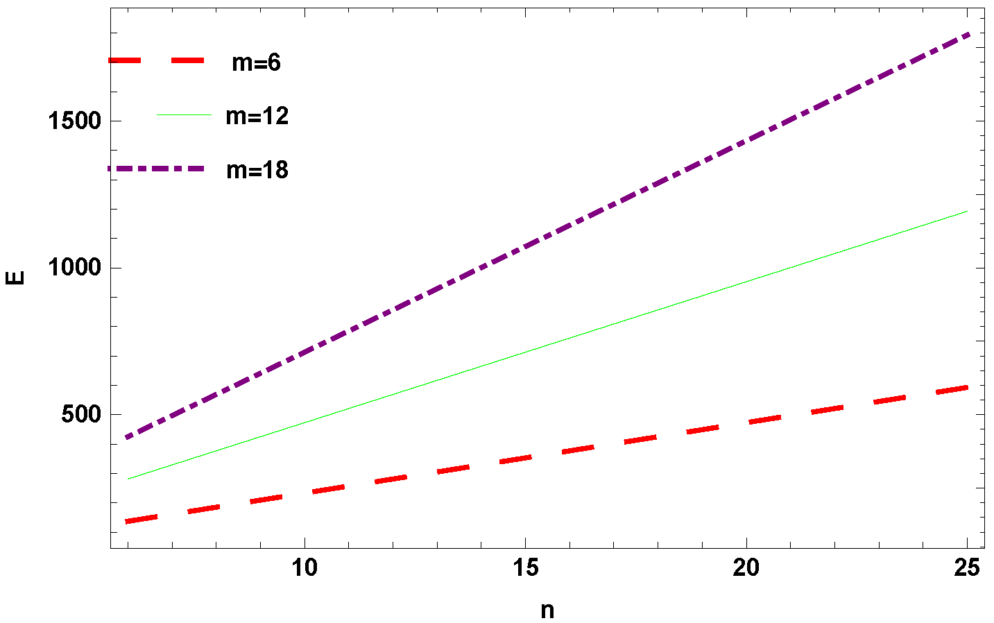
Figure 5 represents increasing behaviour of distance energy with respect to n while keeping m constant. The three different colored lines correspond to three different values of m.

Figure 6 shows that, with the rise in m and n, the values of adjacency energies rise. It is the 3D plot showing trends with changes in both m and n.

Figure 7 represents behaviour of adjacency energy with respect to n while keeping m constant. The three different colored lines correspond to three different values of m.

In this paper, we compute closed forms of distance and adjacency energies of generalized wheels and particularize these for classical wheels. These results are helpful for mathematicians and chemists working in industry as generalized wheels can be considered as particular cyclic structures having a common hub.

References

- Diudea, M.V.; Gutman, I.; Lorentz, J. Molecular Topology; Babes-Bolyai University: Cluj-Napoca, Romania, 1999; ISBN 1-56072-957-0. [Google Scholar]
- Gutman, I.; Kiobucar, A.; Majstrovic, S. Selected Topics from the Theory of Graph Energy: Hypoenergetic Graphs; Applications of Graph Spectra Mathematical Institution: Belgrade, Serbia, 2009; pp. 65–105. [Google Scholar]
- Meenakshi, S.; Lavanya, S. A Survey on Energy of Graphs. Ann. Pure Appl. Math. 2014, 8, 183–191. [Google Scholar]
- Gutman, I. The energy of a graph. Steiermark. Math. Symp. 1978, 103, 1–22. [Google Scholar]
- Jooyandeh, M.; Kiani, D.; Mirzakhah, M. Incidence energy of a graph. MATCH. Commun. Math. Comput. Chem. 2009, 62, 561–572. [Google Scholar]
- Indulal, G.; Vijaykumar, A. Energies of some non-regular graphs. J. Math. Chem. 2007, 42, 377–386. [Google Scholar] [CrossRef]
- Bieri, G.; Dill, J.; Heilbronner, E.; Schmelzer, A. Application of the Equivalent Bond Orbital Model to the C2s-Ionization Energies of Saturated Hydrocarbons. Helv. Chim. Acta 1977, 60, 2234–2247. [Google Scholar] [CrossRef]
- Heilbronner, E. A Simple Equivalent Bond Orbital Model for the Rationalization of the C2s-Photoelectron Spectra of the Higher n-Alkanes, in Particular of Polyethylene. Helv. Chim. Acta 1977, 60, 2248–2257. [Google Scholar] [CrossRef]
- Gunthard, H.; Primas, H. Zusammenhang von Graphentheorie und MO-Theorie von Molekeln mit Systemen konjugierter Bindungen. Helv. Chim. Acta 1956, 39, 1645–1653. [Google Scholar] [CrossRef]
- Gutman, I.; Zhou, B. Laplacian energy of a graph. Lin. Algebra Appl. 2006, 414, 29–37. [Google Scholar] [CrossRef] [Green Version]
- Gutman, I.; Indulal, G.; Vijayakumar, A. On distance energy of graphs. MATCH Commun. Math. Compul. Chen. 2008, 60, 461–472. [Google Scholar]
- Gutman, I.; Li, X.; Shi, Y. Graph Energy; Springer: New York, NY, USA, 2012. [Google Scholar]
- Nikiforov, V. The energy of graphs and matrices. J. Math. Anal. Appl. 2007, 326, 1472–1475. [Google Scholar] [CrossRef] [Green Version]
- Rowlinson, D.C.P.; Simic, K. Signless Laplacians of finite graphs. MATCH Commun. Math. Comput. Chem. 2007, 57, 211–220. [Google Scholar]
- Sandberg, T.O.; Weinberger, C.; Smatt, J.H. Molecular Dynamics on Wood-Derived Lignans Analyzed by Intermolecular Network Theory. Molecules 2018, 23, 1990. [Google Scholar] [CrossRef] [PubMed]
- Liu, J.B.; Pan, X.F.; Hu, F.T. Asymptotic Laplacian-energy-like invariant of lattices. Appl. Math. Comput. 2015, 253, 205–214. [Google Scholar] [CrossRef] [Green Version]
- Liu, J.B.; Pan, X.F. Asymptotic incidence energy of lattices. Physica A 2015, 422, 193–202. [Google Scholar] [CrossRef]
- Zhou, B.; Gutman, I. On Laplacian energy of graphs. MATCH Commun. Math. Comput. Chem. 2007, 57, 211–220. [Google Scholar]
- Aytac, A.; Turaci, T. Vertex vulnerablility parameter of Gear Graphs. Int. J. Found. Comput. Sci. 2011, 22, 1187–1195. [Google Scholar] [CrossRef]
- Tomescu, I.; Javaid, I. Slamin On the partition dimension and connected partition dimension of wheels. Ars Comb. 2007, 84, 311–317. [Google Scholar]
- Turaci, T. The Average Lower 2-domination Number of Wheels Related Graphs and an Algorithm. Math. Comput. Appl. 2016, 21, 29. [Google Scholar] [CrossRef]
- Siddique, H.M.A.; Imran, H. Computing the metric dimension of wheel related graphs. Appl. Math. Comput. 2014, 242, 624–632. [Google Scholar]
- Hussain, Z.; Muqaddas, M.; Munir, M.; Ali, U.; Zahid, A.; Saleem, S. Bounds for partition dimension of m-Wheels. Open Phys. 2018, in press. [Google Scholar]
Figure 1.
An m-level wheel, .
Figure 2.
.
Figure 3.
Figure 4.
View of distance energy of .
Figure 5.
Distance energy of while keeping m constant.
Figure 6.
View of adjacency energy of .
Figure 7.
Adjacency energy of while keeping m constant.
© 2019 by the authors. Licensee MDPI, Basel, Switzerland. This article is an open access article distributed under the terms and conditions of the Creative Commons Attribution (CC BY) license (http://creativecommons.org/licenses/by/4.0/).
Share and Cite
MDPI and ACS Style
Liu, J.-B.; Munir, M.; Yousaf, A.; Naseem, A.; Ayub, K. Distance and Adjacency Energies of Multi-Level Wheel Networks. Mathematics 2019, 7, 43. https://doi.org/10.3390/math7010043
AMA Style
Liu J-B, Munir M, Yousaf A, Naseem A, Ayub K. Distance and Adjacency Energies of Multi-Level Wheel Networks. Mathematics. 2019; 7(1):43. https://doi.org/10.3390/math7010043
Chicago/Turabian StyleLiu, Jia-Bao, Mobeen Munir, Amina Yousaf, Asim Naseem, and Khudaija Ayub. 2019. "Distance and Adjacency Energies of Multi-Level Wheel Networks" Mathematics 7, no. 1: 43. https://doi.org/10.3390/math7010043
Note that from the first issue of 2016, this journal uses article numbers instead of page numbers. See further details here.