Fault-Tolerant Resolvability and Extremal Structures of Graphs

Abstract

In this paper, we consider fault-tolerant resolving sets in graphs. We characterize n-vertex graphs with fault-tolerant metric dimension n, $n-1$, and 2, which are the lower and upper extremal cases. Furthermore, in the first part of the paper, a method is presented to locate fault-tolerant resolving sets by using classical resolving sets in graphs. The second part of the paper applies the proposed method to three infinite families of regular graphs and locates certain fault-tolerant resolving sets. By accumulating the obtained results with some known results in the literature, we present certain lower and upper bounds on the fault-tolerant metric dimension of these families of graphs. As a byproduct, it is shown that these families of graphs preserve a constant fault-tolerant resolvability structure.

1. Introduction

In 1975, Slater [1] introduced the concept of a resolving set and its minimality within the graph, known as the metric dimension. Independently, Harary and Melter [2] proposed the same concept by explaining its diverse applicability. The research on this graph-theoretic parameter is excelling, and hundreds of manuscripts have been published from both theoretic and applicability perspectives. By considering its applicability perspective, the metric dimension significantly possesses many potentially diverse applications in different areas of science, social science, and technology. Next, we discuss applications of the metric dimension in other scientific disciplines.

The emergence and diversity of metric dimension applications prevail in many scientific areas, such as the navigation of robots in robotics [3], determining routing protocols geographically [4], and telecommunication [5]. The vertex–edge relation in graphs and its equivalence to the atom–bond relation derive many applications in chemistry [6]. Network discovery and its verification [5] is another area in which interesting applications of the metric dimension emerge. Based on its importance in other scientific areas, it is natural to study the mathematical properties of this parameter. Next, we review some literature on the mathematical significance of this graph-theoretic parameter.

Various families of graphs of mathematical interest have been studied from the metric dimension perspective. Here, we mention some of the important work: the metric dimension of certain families of distance-regular graphs, such as Grassmann graphs [7] and Johnson graphs [8], which have been studied by Bailey and others. The metric dimension of Kneser graphs was also studied by Bailey at al. [8]. Graphs of group-theoretic interest, such as Cayely digraphs [9] and Cayley graphs generated by certain finite groups [10], have also been studied from the metric dimension viewpoint. The metric dimension and resolving sets of product graphs, such as the Cartesian product of graphs [11] and categorical product of graphs [12], have also been investigated. Certain infinite families generated from wheel graphs have been studied by Siddiqui et al. [13]. The metric dimension of rotationally symmetric convex polytopes (resp. convex polytopes produced by wheel-related graphs) has been studied by Kratica et al. [14] (resp. Imran et al. [15]). The question of whether or not the metric dimension is a finite number was answered in [16]. They showed this result by constructing some infinite families of graphs possessing infinite metric dimension. Similar to many other graph-theoretic parameters, the computational complexity of the metric dimension problem was investigated in [17].

Metric dimension has also been generalized and extended by providing more mathematical rigorous general concepts, such as the k-metric dimension. Hernando et al. [18] introduced another concept: fault tolerance in resolvability, which tolerates the removal of any arbitrary vertex and preserves the resolvability status of the underlying set. By considering the vertices in a resolving set as the location for loran/sonar stations, we can say that the location of any such vertex is distinctly measured by its vertex distances from the site of the stations. From this perspective, a fault-tolerant (unique) resolving set is the one which still preserves the property of a resolving set when neglecting any station at a uniquely determined location of a vertex in the resolving set. Consequently, fault-tolerant resolving sets enhance the applicability of classical resolving sets in graphs. In addition, this shows that the fault-tolerant metric dimension possesses applicative superiority over the metric dimension.

Chartrand [19] investigated certain applications by referring to components of a metric basis as sensors. From the fault-tolerant resolvability point of view, if some sensor is lacking in performance and does not convey information efficiently, the system will not have enough information process in order to tackle the thief/intruder/fire, etc. A fault-tolerant resolving set from this perspective deals with this problem by conveying the information efficiently when one of the sensors does not catch the intruder. It turns out that fault tolerance in resolvability has applicative superiority over classical resolvability in graphs. In other words, the fault-tolerant metric dimension has application wherever the metric dimension is applicable. Nevertheless, fault-tolerant resolving sets have not received much attention from researchers. The fault-tolerant metric dimension of certain interesting graphs possessing chemical importance was studied in [20]. Recently, Raza et al. [21,22] considered certain rotationally symmetric convex polytopes and studied their fault-tolerant metric dimension and binary-locating dominating sets. The reader is referred to [23] for consideration of fault-tolerant resolvability as an optimization problem and its applicative perspective. We also refer the reader to [24,25,26,27,28] for a study of other interesting graph-theoretic parameters having potential applications in chemistry.

Based on the importance of fault-tolerant resolvability from both mathematical and applicative perspectives as discussed above, it is natural to study the mathematical properties of fault-tolerant resolving sets in graphs. In this paper, we study the fault-tolerant resolvability in graphs. We characterize the graphs with fault-tolerant metric dimension n, $n-1$, and 2, which are the non-trivial extremal values of the fault-tolerant metric dimension. We utilize a lemma to trace a fault-tolerant resolving set from a given resolving set. This results in proving a non-trivial upper bound on the fault-tolerant metric dimension of a graph with a given resolving set. We study the fault-tolerant resolvability for three infinite families of regular graphs and show some upper and lower bounds on their fault-tolerant metric dimension.

2. Preliminaries

This section defines the terminologies and explains the undefined terms from the previous section. We also provide an overview of basic results in the literature which are used in subsequent sections. Notations and graph-theoretic concepts were taken from Bondy and Murty [29].

A graph is an ordered pair $\mathsf{\Gamma }=(V,E)$, where V is considered to be the vertex set and E is called the edge set. $\mathsf{\Gamma }$ is called finite if V is finite; it is said to be simple if it does not contain any loop and parallel edges; it is called undirected if its edges do not possess direction; and it is called connected if any two vertices in it are connected by a path. The length of the shortest path between two given vertices is called the distance between them. For $u,v\in V$, the distance between u and v is usually denoted as $d_{u,v}$.

For two arbitrary vertices x and y, a vertex u is said to resolve the pair $x,y$ if it satisfies $d_{u,x}\ne d_{u,y}$. If this resolvability condition is satisfied by a number of vertices composing a subset $R\subseteq V$, i.e., any pair of vertices in the graph is resolved by at least one vertex in R, then L is said to be a resolving set. The idea behind this definition goes back to Harary and Melter [2], who showed that this concept naturally arises from communication networks. The minimum cardinality of a resolving set in a given graph is said to be the metric dimension. It is usually denoted by $\beta \left(G\right)$. A resolving set in which the number of elements is $\beta$ is called the metric basis. For an ordered subset $R=(x_1,x_2,\dots ,x_r)$, the R-coordinate/code/representation of vertex u in V is $C_R\left(u\right)=(d_{u,x_1},d_{u,x_2},\dots ,d_{u,x_r})$. In these terms, L is said to be a resolving set of $\mathsf{\Gamma }$ if any two vertices in $\mathsf{\Gamma }$ have distinct codes or distance vectors.

Chartrand et al. [6] determined all the connected graphs with metric dimension 1. Let $P_{\nu }$ be the $\nu$-vertex path graph.

Theorem 1.

[6] A connected graph has metric dimension 1 if and only if it is the path graph.

They also showed that a graph having metric dimension 2 cannot possess $K_{3,3}$ and $K_5$ as its subgraphs. Let $K_{\nu }$ be the complete graph on $\nu$ vertices. They also classified the connected graphs possessing metric dimension $\nu -1$.

Theorem 2.

[6] A connected ν-vertex graph has metric dimension $\nu -1$ if and only if it is the complete graph.

Let $\mathsf{\Gamma }\cup \Omega$ denote the disjoint union of two graphs $\mathsf{\Gamma }$ and $\Omega$. The join of two graphs $\mathsf{\Gamma }$ and $\Omega$, symbolized as $\mathsf{\Gamma }+\Omega$, is obtained by joining any vertex of $\mathsf{\Gamma }$ to all the vertices of $\Omega$ and vice versa. Graphs having $\nu$ vertices sharing the metric dimension $\nu -2$ are classified in the following result.

Theorem 3.

[6] A connected ν-vertex graph Γ with $\nu \ge 4$ shares the metric dimension $\nu -2$ if and only if $\mathsf{\Gamma }\in \{K_s+\overline{K_t}(s\ge 1,t\ge 2),K_{s,t}(s,t\ge 1),K_s+(K_1\cup K_t)(s,t\ge 1)\}$.

A fault-tolerant resolving set is a resolving set in which the removal of an arbitrary vertex maintains the resolvability. The idea of a fault-tolerant resolving set (also known as resilient) has been widely investigated in networked systems; see, for example, [30,31]. The fault-tolerant metric dimension and fault-tolerant metric basis are defined similarly as metric dimension. We denote the fault-tolerant metric dimension of graph $\mathsf{\Gamma }$ by ${\beta }^{\prime }\left(\mathsf{\Gamma }\right)$.

A family of graphs on $\nu$ vertices is said to possess a constant (resp. bounded) resolvability/fault-tolerant resolvability structure if the metric dimension/fault-tolerant metric dimension does not depend on the parameter $\nu$ (resp. is a function of $\nu$). Note that our definition of a constant/bounded metric/fault-tolerant metric dimension could be different from the one in the literature. In view of Theorem 1, path graphs are a family of graphs with a constant metric dimension. On the other hand, in view of Theorem 2, complete graphs provide a family of graphs possessing a bounded resolvability structure.

In a path graph, there exists a unique fault-tolerant metric basis comprising the initial and terminal vertices. Thus, we obtain ${\beta }^{\prime }\left(P_n\right)=2$. Hernando et al. [18] showed that the tree T in Figure 1 has $\beta \left(T\right)=10$ and ${\beta }^{\prime }\left(T\right)=14$. The set $P=(1,2,3,4,\dots ,10)$ (resp. $Q=P\cup \{y,v,r,s\}$) forms the metric basis (resp. fault-tolerant metric basis) of T.

Javaid et al. proved the following lemma, which shows an alternative way to trace a fault-tolerant resolving set in a graph.

Lemma 1.

[32] A resolving set R of graph Γ is fault-tolerant if and only if any arbitrary pair of vertices of Γ is resolved by at least two vertices of R.

Proof. 

Let R be a fault-tolerant resolving set of G. Assume contrarily that two vertices x and y of G are resolved by a single vertex $r\in R$. Then, $R\setminus \left\{r\right\}$ is not a resolving set since both x and y have the same codes with respect to $r\in R$. This raises a contradiction to the assumption that R is a fault-tolerant resolving set of G.

Now, we assume that every pair of vertices of G is resolved by at least two vertices of R. Then, $R\setminus \left\{r\right\}$ for any $r\in R$ is a resolving set by definition. This shows the lemma. ☐

Hernando et al. [18] showed the following upper bound on ${\beta }^{\prime }$ in terms of $\beta$.

Theorem 4.

[18] The upper bound ${\beta }^{\prime }\left(\mathsf{\Gamma }\right)\le \beta \left(\mathsf{\Gamma }\right)\left(1+2\times 5^{\beta \left(\mathsf{\Gamma }\right)-1}\right)$ holds for any arbitrary graph.

The following result demonstrates that the difference between the two parameters $\beta$ and ${\beta }^{\prime }$ can be increasingly large enough.

Theorem 5.

[32] There always exists a graph Γ for which ${\beta }^{\prime }\left(\mathsf{\Gamma }\right)\ge \beta \left(\mathsf{\Gamma }\right)+p$ holds for any integer p.

From this, we can also note that, with the defining structures of $\beta$ and ${\beta }^{\prime }$, we can have ${\beta }^{\prime }\left(\mathsf{\Gamma }\right)\ge \beta \left(\mathsf{\Gamma }\right)+1$. In the next section, we discuss graphs which hold equality in this lower bound.

3. Main Results

This section contains the main result presented in this paper.

3.1. Some Characterizations

In this subsection, we prove some characterization results on extreme values of the fault-tolerant metric dimension of graphs. These results are the fault-tolerant metric dimension analogs of Theorems 1–3, where similar results on the metric dimension of graphs are obtained. Note that from the interpretation of the fault-tolerant metric dimension of a graph $\mathsf{\Gamma }$ with n vertices, we have $2\le {\beta }^{\prime }\left(\mathsf{\Gamma }\right)\le n$.

In the following result, graphs with fault-tolerant metric dimension 2 are characterized.

Theorem 6.

A graph has ${\beta }^{\prime }\left(\mathsf{\Gamma }\right)=2$ if and only if it is the path graph.

Proof. 

First, we assume that $\mathsf{\Gamma }\cong P_n$. By Theorem 1, we obtain $\beta \left(\mathsf{\Gamma }\right)=1$. By the definition of the fault-tolerant metric dimension, it is noted that

$${\beta }^{\prime }\left(\mathsf{\Gamma }\right)\ge \beta \left(\mathsf{\Gamma }\right)+1.$$

(1)

By inserting $\beta \left(\mathsf{\Gamma }\right)=1$ in Equation (1), we get ${\beta }^{\prime }\left(\mathsf{\Gamma }\right)\ge 2$. Let $R^{\prime }=\{a,b\}\subseteq V\left(\mathsf{\Gamma }\right)$, where a and b are the vertices with degree one in $\mathsf{\Gamma }$. Clearly, $R^{\prime }$ is a resolving set in $\mathsf{\Gamma }$. Note that both $R^{\prime }\setminus \left\{a\right\}$ and $R^{\prime }\setminus \left\{b\right\}$ are also resolving sets in $\mathsf{\Gamma }$, because any vertex of degree one resolves the path graph. This implies that $R^{\prime }$ is a fault-tolerant resolving set of $\mathsf{\Gamma }$, and thus, ${\beta }^{\prime }\left(\mathsf{\Gamma }\right)\le 2$. By combining two inequalities, we obtain ${\beta }^{\prime }(\mathsf{\Gamma }=P_n)=2$.

Conversely, suppose that $\mathsf{\Gamma }$ is a graph with fault-tolerant metric dimension 2. Since both $\beta \left(\mathsf{\Gamma }\right)$ and ${\beta }^{\prime }\left(\mathsf{\Gamma }\right)$ are positive integers, by Equation (1), we get $\beta \left(\mathsf{\Gamma }\right)<{\beta }^{\prime }\left(\mathsf{\Gamma }\right)$. By implying ${\beta }^{\prime }\left(\mathsf{\Gamma }\right)=2$, we obtain $\beta \left(\mathsf{\Gamma }\right)<2$, which indicates that $\beta \left(\mathsf{\Gamma }\right)=1$. By Theorem 1, we find that the only graphs with metric dimension 1 are the path graphs. This implies that $\mathsf{\Gamma }\cong P_n$. ☐

In the next theorem, we characterize the equality in ${\beta }^{\prime }\left(\mathsf{\Gamma }\right)\le n$, where $\mathsf{\Gamma }$ is an n-ordered graph.

Theorem 7.

An n-vertex connected graph has ${\beta }^{\prime }\left(\mathsf{\Gamma }\right)=n$ if and only if it is the complete graph $K_n$.

Proof. 

Let $\mathsf{\Gamma }$ be an n-ordered complete graph. Then, by Theorem 2, we have $\beta \left(\mathsf{\Gamma }\right)=n-1$. By putting this in Equation (1), we get ${\beta }^{\prime }\left(\mathsf{\Gamma }\right)\ge n$. Let $R^{\prime }=V\left(\mathsf{\Gamma }\right)$; for some $c\in V\left(\mathsf{\Gamma }\right)$, the set $R^{\prime }\setminus \left\{c\right\}$ is a resolving set, because any collection of $n-1$ vertices of $\mathsf{\Gamma }$ resolve $\mathsf{\Gamma }$ completely. Thus, $R^{\prime }$ is a fault-tolerant resolving set of $\mathsf{\Gamma }$, and thus, ${\beta }^{\prime }\left(\mathsf{\Gamma }\right)\le n$. By combining these two cases, we obtain ${\beta }^{\prime }\left(\mathsf{\Gamma }\right)=n$.

Conversely, suppose that $\mathsf{\Gamma }$ is a graph with fault-tolerant metric dimension n. From Equation (1), we have $\beta \left(\mathsf{\Gamma }\right)<{\beta }^{\prime }\left(\mathsf{\Gamma }\right)$, which shows that $\beta \left(\mathsf{\Gamma }\right)\le n-1$. In Theorem 2, it is shown that equality holds in $\beta \left(\mathsf{\Gamma }\right)\le n-1$ if and only if $\mathsf{\Gamma }=K_n$. This shows that equality holds in $\beta \left(\mathsf{\Gamma }\right)\le {\beta }^{\prime }\left(\mathsf{\Gamma }\right)-1=n-1$. This implies that $\mathsf{\Gamma }$ is a complete graph on n vertices. ☐

In the next theorem, graphs with fault-tolerant metric dimension $n-1$ are characterized.

Theorem 8.

Let Γ be a graph with order $n\ge 4$. Then, ${\beta }^{\prime }\left(\mathsf{\Gamma }\right)=n-1$ if and only if $\mathsf{\Gamma }=K_{s,t}(s,t\ge 1)$, $\mathsf{\Gamma }=K_s+\overline{K_t}(s\ge 1,t\ge 2)$ and $\mathsf{\Gamma }=K_s+(K_1\cup K_t)(s,t\ge 1)$.

Proof. 

Let ${\mathsf{\Gamma }}_1=K_{s,t}(s,t\ge 1)$, ${\mathsf{\Gamma }}_2=K_s+\overline{K_t}(s\ge 1,t\ge 2)$, and ${\mathsf{\Gamma }}_3=K_s+(K_1\cup K_t)(s,t\ge 1)$. Assume that $\mathsf{\Gamma }$ belongs to one of the three infinite families ${\mathsf{\Gamma }}_i$, $i=1,2,3$. Then, by Theorem 3, $\beta \left(\mathsf{\Gamma }\right)=n-2$. By using this in Inequality (1), we get ${\beta }^{\prime }\left(\mathsf{\Gamma }\right)\ge n-1$. Since $\mathsf{\Gamma }$ is not a complete graph, by Theorem 7, we obtain ${\beta }^{\prime }\left(\mathsf{\Gamma }\right)<n$. This implies that ${\beta }^{\prime }\left(\mathsf{\Gamma }\right)\le n-1$. Now, we combine the two inequalities to achieve ${\beta }^{\prime }\left(\mathsf{\Gamma }\right)=n-1$.

Conversely, when we let $\mathsf{\Gamma }$ be a graph with fault-tolerant metric dimension $n-1$, by using Equation (1), ${\beta }^{\prime }\left(\mathsf{\Gamma }\right)\ge \beta \left(G\right)+1$ implies

$$\beta \left(\mathsf{\Gamma }\right)\le n-2.$$

(2)

By Theorem 3, equality holds in Equation (2) if $\mathsf{\Gamma }\in \{{\mathsf{\Gamma }}_1,{\mathsf{\Gamma }}_2,{\mathsf{\Gamma }}_3\}$, if $n\ge 4$. This implies that the equality holds in $\beta \left(\mathsf{\Gamma }\right)\le {\beta }^{\prime }\left(\mathsf{\Gamma }\right)-1$, and thus, for $n\ge 4$, $\mathsf{\Gamma }\in {\mathsf{\Gamma }}_i$ for $i=1,2,3$. This completes the proof. ☐

By Theorems 6–8, if $\mathsf{\Gamma }$ is a graph with $\mathsf{\Gamma }\notin \{P_n,K_n,{\mathsf{\Gamma }}_1,{\mathsf{\Gamma }}_2,{\mathsf{\Gamma }}_3\}$, then $3\le {\beta }^{\prime }\left(\mathsf{\Gamma }\right)\le n-2$. Next, we focus on the graphs for which $3\le {\beta }^{\prime }\left(\mathsf{\Gamma }\right)\le n-2$.

3.2. Relation between Resolving Sets and Fault-Tolerant Resolving Sets of Graphs

In Theorem 4, Hernando et al. [18] showed that the fault-tolerant metric dimension is bounded by a function of metric dimension. They also showed a relation between a resolving set and a fault-tolerant resolving set for an arbitrary graph. Now, let $N\left(w\right)$ (resp. $N\left[w\right]$) represent the open and close neighborhood of a vertex $w\in V\left(\mathsf{\Gamma }\right)$, where $N\left(w\right):=\{u\in V(\mathsf{\Gamma })\mid uw\in E(\mathsf{\Gamma }\left)\right\}$ and $N\left[w\right]:=\left\{w\right\}\cup N\left(w\right)$.

Lemma 2.

[18] Let R be a resolving set of graph Γ. For all $w\in R$, let $T\left(w\right):=\{x\in V(\mathsf{\Gamma }):N(w)\subseteq N(x\left)\right\}$. Then, $R^{\prime }:={\cup }_{w\in R}(N\left[w\right]\cup T\left(w\right))$ is a fault-tolerant resolving set of Γ.

Now, the following lemma will help us to obtain upper bounds on the fault-tolerant metric dimension of a given graph. It uses R in a graph to produce a fault-tolerant resolving set within it. In view of Lemma 2, for a given resolving set R of a graph $\mathsf{\Gamma }$, finding the set $R^{\prime }$ to evaluate the corresponding fault-tolerant resolving set seems tedious due to the calculation of the set $T\left(w\right)$ for a vertex $w\in R$. Raza et al. [21] further simplify this lemma so that one does not have to check every vertex x of $\mathsf{\Gamma }$ to verify whether or not it belongs to $T\left(w\right)$ for some $w\in R$. Now, for vertices x and y in $\mathsf{\Gamma }$, we let $\lambda (x,y)$ be a set of common neighbors of these vertices and, for some $Q\subset V\left(\mathsf{\Gamma }\right)$, let $\lambda \left(Q\right)$ be the set of common neighbors of each vertex in Q. The following lemma is a key result for finding upper bounds on the fault-tolerant metric dimension of a given graph.

Lemma 3.

[21] For a graph Γ, let R be a distinguishing or resolving set, and $R^{\prime }:={\cup }_{w\in R}\left(N\left[w\right]\cup \lambda \left(N\right(w\left)\right)\right)$. Then, ${\beta }^{\prime }\left(G\right)\le \mid R^{\prime }\mid$.

Proof. 

Let R be a resolving set of graph $\mathsf{\Gamma }$. For $v\in R$, let $T\left(v\right):=\{x\in V(\mathsf{\Gamma }):N(v)\subseteq N(x\left)\right\}$. Then, for any $x\in T\left(v\right)$, we notice that $d(x,v)=2$ (see Figure 2).

Moreover, for $y,z\in N\left(v\right)$, we obtain $\lambda (y,z)=x$ for some $x\in T\left(v\right)$. This implies that $T\left(v\right)=\lambda \left(N\left(v\right)\right)\setminus \left\{v\right\}$ for any $v\in R$. Now, by Lemma 2, $R^{\prime }:={\cup }_{v\in R}(N\left[v\right]\cup T\left(v\right))$ is a fault-tolerant resolving set of $\mathsf{\Gamma }$. Since v is contained in $N\left[v\right]$, then, for any $v\in R$,

$$N\left[v\right]\cup T\left(v\right)=N\left[v\right]\cup \lambda \left(N\left(v\right)\right).$$

This shows the lemma. ☐

We use Lemma 3 in later subsections to calculate upper bounds on the fault-tolerant metric dimension for certain families of regular graphs.

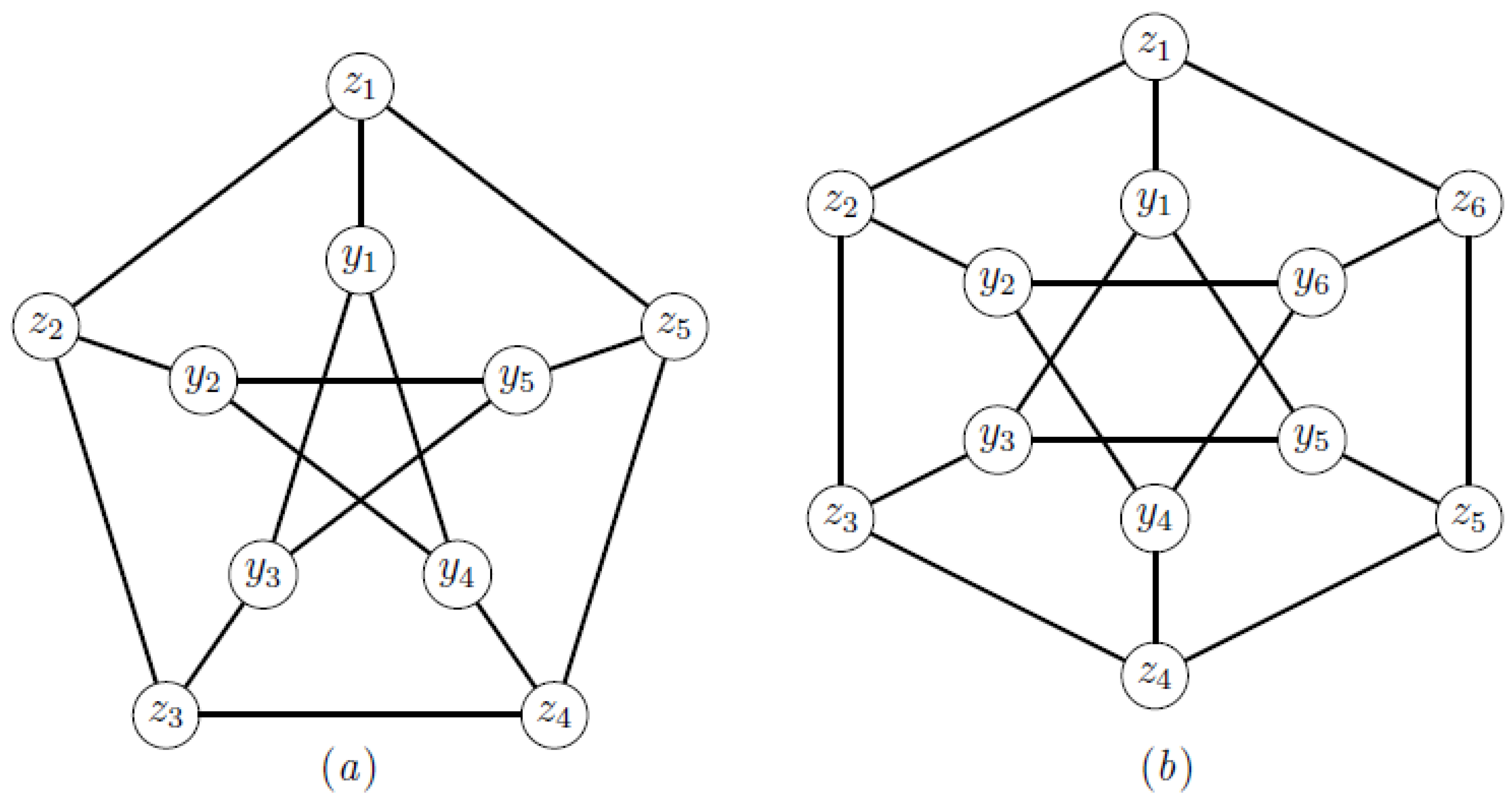
3.3. Extended Petersen Graphs

The extended Petersen graph $P\left(n\right)$, $n\ge 3$, has a vertex set

$$V=\{z_1,z_2,\dots z_n,y_1,y_2,\dots y_n\}$$

and an edge set

$$E=\{z_i{z}_{i+1},z_i{y}_i,y_i{y}_{i+2}|\mathrm{with}\mathrm{indices}\mathrm{taken}\mathrm{as}\mathrm{modulo}n\}.$$

The extended Petersen graph $P\left(n\right)$ is a special case of the generalized Petersen graphs which were first studied by Watkins [33].

We studied the problem of the fault-tolerant metric dimension of the extended Petersen graph. The set $\{z_1,z_2,\dots ,z_n\}$ prompts a cycle in $P\left(n\right)$, with $z_k{z}_{k+1}(1\le k\le n)$ and $y_k{y}_{k+2}(1\le k\le n)$, with indices taken modulo n, as edges. For even n, $\{y_1,y_2,\dots ,y_n\}$ induces two cycles, again with edges $y_k{y}_{k+2}$$(1\le k\le n)$, with indices taken modulo n. For example, $P\left(5\right)$ is the standard Petersen graph. For the sake of simplicity, we denote the cycle induced by $\{z_1,z_2,\dots ,z_n\}$ as the outer cycle and the cycle induced by $\{y_1,y_2,\dots ,y_n\}$ as the inner cycle or cycles.

The following result was shown by Javaid et al. [34].

Proposition 1.

[34] Let Γ be the extended Petersen graph $P\left(n\right)$ with $n\ge 5$; then, $\beta \left(\mathsf{\Gamma }\right)=3$.

They also showed the following:

Proposition 2.

[34] $P\left(n\right)$, the extended Petersen graph, can be classified as a family of graphs with a constant metric dimension.

In this section, we present our main results. We derive the upper as well as lower bounds on the fault-tolerant metric dimension of the extended Petersen graph $P\left(n\right)$. Note that Claim 1 in the following result was essentially shown in Proposition 1.

Theorem 9.

Let Γ be the extended Petersen graph $P\left(n\right)$; then,

$$4\le {\beta }^{\prime }\left(\mathsf{\Gamma }\right)\le \left\{\begin{array}{cc}10,\hfill & ifn\equiv 0(mod2)withn\ge 8;\hfill \\ 12,\hfill & ifn\equiv 1(mod2)withn\ge 11.\hfill \end{array}\right.$$

Proof. 

Let $\mathsf{\Gamma }$ be the extended Petersen graph $P\left(n\right)$, with $n\ge 4$.

Case 1: When $n\equiv 0(mod2)$ with $n\ge 8$.

Claim 1: Resolving set R of order 3 exists in $\mathsf{\Gamma }$.

Based on the location of basis elements in $\mathsf{\Gamma }$, we further divide this case into two subcases.

Subcase 1.1: When $n\equiv 0(mod4)$.

It can be written as $n=4\ell$, $2\le \ell \in {\mathbb{Z}}^{+}$. We prove that $R=\{y_1,y_2,y_3\}$ resolves $V\left(\mathsf{\Gamma }\right)$. In order to show that R resolves vertices of $V\left(\mathsf{\Gamma }\right)$, we first represent the vertices in $\mathsf{\Gamma }$ with respect to $R\setminus \left\{y_3\right\}$. Indeed, the vertices $y_1$ and $y_2$ distinguish the inner cycle vertices and a few of the outer cycle vertices. The vertices in the outer cycle are represented by $C_{R\setminus \left\{y_3\right\}}\left(z_1\right)=(1,2)$, $C_{R\setminus \left\{y_3\right\}}\left(z_2\right)=(2,1)$,

$$C_{R\setminus \left\{y_3\right\}}\left(z_{2k}\right)=\left\{\begin{array}{cc}(k+1,k),\hfill & 2\le k\le \ell ;\hfill \\ (2\ell -k+2,2\ell -k+2),\hfill & \ell +1\le k\le 2\ell .\hfill \end{array}\right.$$

$$C_{R\setminus \left\{y_3\right\}}\left(z_{2k+1}\right)=\left\{\begin{array}{cc}(k+1,k+1),\hfill & 1\le k\le \ell ;\hfill \\ (2\ell -k+1,2\ell -k+2),\hfill & \ell +1\le k\le 2\ell -1.\hfill \end{array}\right.$$

In the inner cycle,

$$C_{R\setminus \left\{y_3\right\}}\left(y_{2k}\right)=\left\{\begin{array}{cc}(k+2,k-1),\hfill & 2\le k\le \ell ;\hfill \\ (2\ell -k+3,2\ell -k+1),\hfill & \ell +1\le k\le 2\ell .\hfill \end{array}\right.$$

and

$$C_{R\setminus \left\{z_3\right\}}\left(y_{2k+1}\right)=\left\{\begin{array}{cc}(k,k+2),\hfill & 1\le k\le \ell ;\hfill \\ (2\ell -k,2\ell -k+3),\hfill & \ell +1\le k\le 2\ell -1.\hfill \end{array}\right.$$

From the above discussion, it is clear that there are no two vertices with the same representation in the inner cycle. However, in the outer cycle, $C_{R\setminus \left\{y_3\right\}}\left(z_{3+k}\right)=C_{R\setminus \left\{y_3\right\}}\left(z_{n-k}\right)$ for $k=0,2,\dots ,2\ell -2$. Vertex $y_3$ distinguishes these pairs with the same representation as $d(y_3,z_{3+k})=\lfloor \frac{3+k}{2}\rfloor \ne d(y_3,z_{n-k})=\lfloor \frac{3+k}{2}\rfloor +2$ for $k=0,2,\dots ,2\ell -4$ and $d(y_3,z_{2\ell +2})=d(y_3,z_{2\ell +1})+1$. This shows that R resolves vertices of $\mathsf{\Gamma }$, which means $\beta \left(\mathsf{\Gamma }\right)\le 3$ when $n\equiv 0(mod4)$.

Subcase 1.2: When $n\equiv 2(mod4)$.

It can be written as $n=4\ell +2$, $2\le \ell \in {\mathbb{Z}}^{+}$. In this case, again, $R=\{y_1,y_2,y_3\}$ resolves $V\left(\mathsf{\Gamma }\right)$. In order to show that R resolves the vertices of $V\left(P\right(n\left)\right)$, we first represent the vertices in $\mathsf{\Gamma }$ with respect to $R\setminus \left\{y_3\right\}$. Again, it is clear that the vertices $y_1$ and $y_2$ distinguish the inner and outer cycle vertices. Note that for the outer cycle, we have $C_{R\setminus \left\{y_3\right\}}\left(z_1\right)=(1,2)$, $C_{R\setminus \left\{y_3\right\}}\left(z_2\right)=(2,1)$,

$$C_{R\setminus \left\{y_3\right\}}\left(z_{2k}\right)=\left\{\begin{array}{cc}(k+1,k),\hfill & 2\le k\le \ell +1;\hfill \\ (2\ell -k+3,2\ell -k+3),\hfill & \ell +2\le k\le 2\ell +1.\hfill \end{array}\right.$$

and

$$C_{R\setminus \left\{y_3\right\}}\left(z_{2k+1}\right)=\left\{\begin{array}{cc}(k+1,k+1),\hfill & 1\le k\le \ell ;\hfill \\ (2\ell -k+2,2\ell -k+3),\hfill & \ell +1\le k\le 2\ell .\hfill \end{array}\right.$$

In the inner cycle,

$$C_{R\setminus \left\{y_3\right\}}\left(y_{2k}\right)=\left\{\begin{array}{cc}(k+2,k-1),\hfill & 2\le k\le \ell +1;\hfill \\ (2\ell -k+4,2\ell -k+2),\hfill & \ell +2\le k\le 2\ell +1.\hfill \end{array}\right.$$

and

$$C_{R\setminus \left\{y_3\right\}}\left(y_{2k+1}\right)=\left\{\begin{array}{cc}(k,k+2),\hfill & 1\le k\le \ell ;\hfill \\ (2\ell -k+1,2\ell -k+4),\hfill & \ell +1\le k\le 2\ell .\hfill \end{array}\right.$$

Again, in this case, it is clear for the inner cycle that there are no two vertices with the same representation. However, for the outer cycle, $C_{R\setminus \left\{y_3\right\}}\left(z_{3+k}\right)=C_{R\setminus \left\{y_3\right\}}\left(z_{n-k}\right)$ for $k=0,2,\dots ,2\ell -2$. Note that the pairs with the same representations are distinguished by $y_3$ since $d(y_3,z_{3+k})=\lfloor \frac{3+k}{2}\rfloor \ne d(y_3,z_{n-k})=\lfloor \frac{3+k}{2}\rfloor +2$ for $k=0,2,\dots ,2\ell -2$. This shows that R resolves the vertices of $\mathsf{\Gamma }$, which means $\beta \left(\mathsf{\Gamma }\right)\le 3$, when $n\equiv 2(mod4)$.

Claim 2: When $n\ge 8$, the cardinality of the fault-tolerant resolving set in $\mathsf{\Gamma }$ is 10.

We can write $n=4\ell$, $\ell \ge 2$, $\ell \in {\mathbb{Z}}^{+}$. Note that, for this, $R=\{y_1,y_2,y_3\}$ is a resolving set of $\mathsf{\Gamma }$. We show that $\mathsf{\Gamma }$ has a fault-tolerant resolving set of cardinality 10.

As seen from Figure 3, it can be observed that $N\left[y_1\right]=\{y_1,y_3,y_{n-1},z_1\}$, $N\left[y_2\right]=\{y_2,y_4,y_n,z_2\}$, and $N\left[y_3\right]=\{y_1,y_3,y_5,z_3\}$. Moreover, we find that $\lambda \left(N_{\mathsf{\Gamma }}\left(y_1\right)\right)=\lambda \left(N_{\mathsf{\Gamma }}\left(y_2\right)\right)=\lambda \left(N_{\mathsf{\Gamma }}\left(y_3\right)\right)=\varnothing$. Thus, by using Lemma 3, we find that $R^{\prime }=\{y_1,y_2,y_3,y_4,y_5,y_{n-1},y_n,z_1,z_2,z_3\}$ is a fault-tolerant resolving set of $\mathsf{\Gamma }$. Thus, a fault-tolerant resolving set of $\mathsf{\Gamma }$ with cardinality 10 exists when $n\ge 8$.

Case 2: When $n\equiv 1(mod2)$ with $n\ge 11$.

Based on the location of basis elements in $\mathsf{\Gamma }$, we further divide this case into two subcases.

Subcase 2.1: When $n\equiv 1(mod4)$.

Claim 1:$\mathsf{\Gamma }$ has a resolving set R of order 3.

In this case, we can write $n=4\ell +1$, $1\le \ell \in {\mathbb{Z}}^{+}$. It can be seen that $\{y_1,y_2,z_3\}$ is a resolving set for the standard Petersen graph $P\left(5\right)$. For $P\left(9\right)$, we see that $W=\{y_1,y_2,z_4\}$ is a resolving set. Now, we show that, for $n\ge 9$, $R=\{y_1,y_2,z_{2\ell -1}\}$ resolves the vertices of $\mathsf{\Gamma }$, where $n\equiv 1(mod4)$. In order to show this, first we present representations of the vertices with respect to $R\setminus \left\{z_{2\ell -1}\right\}$. The representations of the vertices in the outer cycle are $C_{R\setminus \left\{z_{2\ell -1}\right\}}\left(z_1\right)=(1,2)$, $C_{R\setminus \left\{z_{2\ell -1}\right\}}\left(z_2\right)=(2,1)$,

$$C_{R\setminus \left\{z_{2\ell -1}\right\}}\left(z_{2k}\right)=\left\{\begin{array}{cc}(k+1,k),\hfill & 2\le k\le \ell ;\hfill \\ (k,k),\hfill & k=\ell +1;\hfill \\ (2\ell -k+2,2\ell -k-3),\hfill & \ell +2\le k\le 2\ell .\hfill \end{array}\right.$$

and

$$C_{R\setminus \left\{z_{2\ell -1}\right\}}\left(z_{2k+1}\right)=\left\{\begin{array}{cc}(k+1,k+1),\hfill & 1\le k\le \ell ;\hfill \\ (2\ell -k+2,2\ell -k+2),\hfill & \ell +1\le k\le 2\ell .\hfill \end{array}\right.$$

Now, the representations of the vertices in the inner cycle are

$$C_{R\setminus \left\{y_{z_{2\ell -1}}\right\}}\left(y_{2k}\right)=\left\{\begin{array}{cc}(k+2,k-1),\hfill & 2\le k\le \ell -1;\hfill \\ (k+1,k-1),\hfill & k=\ell ;\hfill \\ (k-1,k-1),\hfill & k=\ell +1;\hfill \\ (k-3,k-1),\hfill & k=\ell +2;\hfill \\ (2\ell -k+1,2\ell -k+4),\hfill & \ell +3\le k\le 2\ell .\hfill \end{array}\right.$$

and

$$C_{R\setminus \left\{z_{2\ell -1}\right\}}\left(y_{2k+1}\right)=\left\{\begin{array}{cc}(k,k+2),\hfill & 1\le k\le \ell -1;\hfill \\ (k,k+1),\hfill & k=\ell ;\hfill \\ (k,k-1),\hfill & k=\ell +1;\hfill \\ (2\ell -k+3,2\ell -k+1),\hfill & \ell +2\le k\le 2\ell .\hfill \end{array}\right.$$

From the above discussion, it is clear that $R\setminus \left\{z_{2\ell -1}\right\}$ distinguishes all but the following vertices. (i) $z_{3+k}$ and $z_{n-k}$ for $i=0,2,\dots ,2\ell -6$. (ii) $z_{2\ell -1}$ and $z_{2\ell +5}$ and $y_{2\ell +2}$. (iii) $z_{2\ell +1}$ , $z_{2\ell +2}$, and $z_{2\ell +3}$. (iv) $y_{2\ell -1}$ and $y_{2\ell +4}$. (v) $y_{2\ell }$ and $y_{2\ell +5}$. (vi) $z_{2\ell }$ and $y_{2\ell +3}$. (vii) $y_{2\ell +1}$ and $z_{2\ell +4}$. It is easy to see that vertices with the same representation in the outer cycle are at different distances from $z_{2\ell -1}.d(z_{2\ell -1},z_{2\ell +5})=5$ and $d(z_{2\ell -1},y_{2\ell +2})=3$, $d(z_{2\ell -1},y_{2\ell -1})=1$ and $d(z_{2\ell -1},y_{2\ell +4})=4$, $d(z_{2\ell -1},y_{2\ell })=2$ and $d(z_{2\ell -1},y_{2\ell +5})=4$, $d(z_{2\ell -1},z_{2\ell })=1$ and $d(z_{2\ell -1},y_{2\ell +3})=3$, $d(z_{2\ell -1},y_{2\ell +1})=2$ and $d(z_{2\ell -1},z_{2\ell +4})=5$. The above discussion shows that R is a resolving set for $V\left(\mathsf{\Gamma }\right)$ when $n\equiv 1(mod4)$. Hence, $\beta \left(\mathsf{\Gamma }\right))\le 3$ for $n\equiv 1(mod4)$.

Claim 2:$\mathsf{\Gamma }$ has a fault-tolerant resolving set of cardinality 12 when $n\ge 11$.

We can write $n=4\ell +1$, $\ell \ge 3$ and $\ell \in {\mathbb{Z}}^{+}$. Note that, in this case, $R=\{y_1,y_2,z_{2\ell -1}\}$ is a resolving set of $\mathsf{\Gamma }$. We prove here that $\mathsf{\Gamma }$ has a fault-tolerant resolving set of cardinality 12. From Figure 3, it can be observed that $N\left[y_1\right]=\{y_1,y_{n-1},y_n,z_1\}$, $N\left[y_2\right]=\{y_2,y_4,y_n,z_2\}$ and $N\left[z_{2\ell -1}\right]=\{z_{2\ell -2},z_{2\ell -1},z_{2\ell },y_{2\ell -1}\}$. Moreover, we find that $\lambda \left(N_{\mathsf{\Gamma }}\left(y_1\right)\right)=\lambda \left(N_{\mathsf{\Gamma }}\left(y_2\right)\right)=\lambda \left(N_{\mathsf{\Gamma }}\left(z_{2\ell -1}\right)\right)=\varnothing$. Thus, by using Lemma 3, we find that $R^{\prime }=\{y_1,y_2,y_3,y_4,y_{2\ell -1},y_{n-1},y_n,z_1,z_2,z_{2\ell -2},z_{2\ell -1},z_{2\ell }\}$ is a fault-tolerant resolving set of $\mathsf{\Gamma }$. Thus, there exists a fault-tolerant resolving set of $\mathsf{\Gamma }$ with cardinality 12.

Subcase 2.2: When $n\equiv 3(mod4)$.

Claim 1: Resolving set R of order 3 in $\mathsf{\Gamma }$ exists.

We can write $n=4\ell +3$, $1\le \ell \in {\mathbb{Z}}^{+}$. It is not difficult to see that $U=\{y_1,y_2,z_3\}$ resolves $V\left(P\right(7\left)\right)$. For $n\equiv 3(mod4)$ and $n\ge 11$, we show that $R=\{y_1,y_2,z_{2\ell +1}\}$ resolves $V(\mathsf{\Gamma }=P(n\left)\right)$. Representations of the vertices in the outer cycle are $C_{R\setminus \left\{z_{2\ell +1}\right\}}\left(z_1\right)=(1,2)$, $C_{R\setminus \left\{z_{2\ell +1}\right\}}\left(z_2\right)=(2,1)$,

$$C_{R\setminus \left\{z_{2\ell +1}\right\}}\left(z_{2k}\right)=\left\{\begin{array}{cc}(k+1,k),\hfill & 2\le k\le \ell +1;\hfill \\ (2\ell -k+3,2\ell -k+4),\hfill & \ell +2\le k\le 2\ell +1.\hfill \end{array}\right.$$

and

$$C_{R\setminus \left\{z_{2\ell +1}\right\}}\left(z_{2k+1}\right)=\left\{\begin{array}{cc}(k+1,k+1),\hfill & 1\le k\le \ell +1;\hfill \\ (2\ell -k+3,2\ell -k+3),\hfill & \ell +2\le k\le 2\ell +1.\hfill \end{array}\right.$$

Now, in the inner cycle,

$$C_{R\setminus \left\{z_{2\ell +1}\right\}}\left(y_{2k}\right)=\left\{\begin{array}{cc}(k+2,k-1),\hfill & 2\le k\le \ell ;\hfill \\ (k,k-1),\hfill & k=\ell +1;\hfill \\ (k-2,k-1),\hfill & k=\ell +2;\hfill \\ (2\ell -k+2,2\ell -k+5),\hfill & \ell +3\le k\le 2\ell +1.\hfill \end{array}\right.$$

and

$$C_{R\setminus \left\{z_{2\ell +1}\right\}}{(}_{2k+1})=\left\{\begin{array}{cc}(k,k+2),\hfill & 1\le k\le \ell ;\hfill \\ (k,k),\hfill & k=\ell +1;\hfill \\ (2\ell -k+4,2\ell -k+2),\hfill & \ell +2\le k\le 2\ell +1.\hfill \end{array}\right.$$

Again, in this case, $R\setminus \left\{z_{2\ell +1}\right\}$ distinguishes all the vertices in $\mathsf{\Gamma }$ except the following vertices: (i) $z_{3+i}$ and $z_{n-i}$ for $i=0,2,\dots ,2\ell -4$. (ii) $z_{2\ell }$, $y_{2\ell +2}$. (iii) $z_{2\ell +1}$, $z_{2\ell +5}$, and $y_{2\ell +3}$. (iv) $y_{2\ell +4}$ and $z_{2\ell +6}$. It is easy to see that vertices with same representation in the outer cycle are at different distances from $z_{2\ell +1}.d(z_{2\ell +1},z_{2\ell })=1$, $d(z_{2\ell +1},y_{2\ell +2})=2$ and $d(z_{2\ell +1},z_{2\ell +5})=4$, $d(z_{2\ell +1},y_{2\ell +3})=2$ and $d(z_{2\ell +1},y_{2\ell +4})=3$, $d(z_{2\ell +1},y_{2\ell +6})=5$. The above discussion shows that R is a resolving set for $V\left(\mathsf{\Gamma }\right)$ when $n\equiv 3(mod4)$ and $n\ge 11$. Hence, $\beta \left(\mathsf{\Gamma }\right)\le 3$ for $n\equiv 3(mod4)$.

Claim 2:$\mathsf{\Gamma }$ has a fault-tolerant resolving set of cardinality 12 with $n\ge 11$.

We can write $n=4\ell +3$, $\ell \ge 2$, $\ell \in {\mathbb{Z}}^{+}$. Note that, in this case, $R=\{y_1,y_2,z_{2\ell +1}\}$ is a resolving set of $\mathsf{\Gamma }$.

We show that $\mathsf{\Gamma }$ has a fault-tolerant resolving set of cardinality 12.

From Figure 3, it can be observed that $N\left[y_1\right]=\{y_1,y_3,y_{n-1},z_1\}$, $N\left[y_2\right]=\{y_2,y_4,y_n,z_2\}$, and $N\left[z_{2\ell +1}\right]=\{z_{2\ell },z_{2\ell +1},z_{2\ell +2},y_{2\ell +1}\}$. Moreover, we find that $\lambda \left(N_{\mathsf{\Gamma }}\left(y_1\right)\right)=\lambda \left(N_{\mathsf{\Gamma }}\left(y_2\right)\right)=\lambda \left(N_{\mathsf{\Gamma }}\left(z_{2\ell +1}\right)\right)=\varnothing$. Thus, by using Lemma 3, we find that $R^{\prime }=\{y_1,y_2,y_3,y_4,y_{n-1},y_n,y_{2\ell +1},z_1,z_2,z_{2\ell },z_{2\ell +1},z_{2\ell +2}\}$ is a fault-tolerant resolving set of $P_{n,2}$. Thus, a fault-tolerant resolving set of $P_{n,2}$ with cardinality 12 exists.

By using Proposition 1, the above discussion, and Inequality (1), we find that ${\beta }^{\prime }\left(\mathsf{\Gamma }\right)\ge 4$. ☐

As a consequence of Theorem 9, we have the following corollary. It provides a fault-tolerant metric dimension analog of Proposition 2.

Corollary 1.

The extended Petersen graph $P\left(n\right)$ is a family of graphs with a constant fault-tolerant metric dimension.

Proof. 

By Theorem 9, we have

$$4\le {\beta }^{\prime }\left(P\left(n\right)\right)\le \left\{\begin{array}{cc}10,\hfill & ifn\equiv 0(mod2)withn\ge 8;\hfill \\ 12,\hfill & ifn\equiv 1(mod2)withn\ge 11.\hfill \end{array}\right.$$

This implies that the fault-tolerant metric dimension of $P\left(n\right)$ does not depend on the defining parameter n. Thus, by definition, $P\left(n\right)$ is a family of graphs with a constant fault-tolerant metric dimension. ☐

In view of Lemma 3 and Proposition 1, we find enough reasoning to propose the following conjecture on the greatest lower bound of the fault-tolerant metric dimension for the extended Petersen graph $P\left(n\right)$.

Conjecture 1.

Let $\mathsf{\Gamma }$ be the extended Petersen graph $P\left(n\right)$; then,

$${\beta }^{\prime }\left(\mathsf{\Gamma }\right)\ge \left\{\begin{array}{cc}10,\hfill & ifn\equiv 0(mod2)withn\ge 8;\hfill \\ 12,\hfill & ifn\equiv 1(mod2)withn\ge 11,\hfill \end{array}\right.$$

and thus, we have

$${\beta }^{\prime }\left(\mathsf{\Gamma }\right)=\left\{\begin{array}{cc}10,\hfill & ifn\equiv 0(mod2)withn\ge 8;\hfill \\ 12,\hfill & ifn\equiv 1(mod2)withn\ge 11.\hfill \end{array}\right.$$

3.4. Anti-Prism Graphs

The cross product of a cycle $C_n$ and $P_2$ is actually called a prism, usually denoted by $D\left(n\right)$. In [11], it was shown that

$$\beta (P_m\square C_n)=\left\{\begin{array}{cc}2,\hfill & \mathrm{if}n\mathrm{is}\mathrm{odd};\hfill \\ 3,\hfill & \mathrm{if}n\mathrm{is}\mathrm{even}.\hfill \end{array}\right.$$

This implies that

$$\beta \left(D\left(n\right)\right)=\left\{\begin{array}{cc}2,\hfill & \mathrm{if}n\mathrm{is}\mathrm{odd};\hfill \\ 3,\hfill & \mathrm{if}n\mathrm{is}\mathrm{even}.\hfill \end{array}\right.$$

By applying Equation (1) and Theorem 4 to the prism graph $D\left(n\right)$, we find the following result.

Proposition 3.

The prism graph $D\left(n\right)$ has a constant fault-tolerant metric dimension.

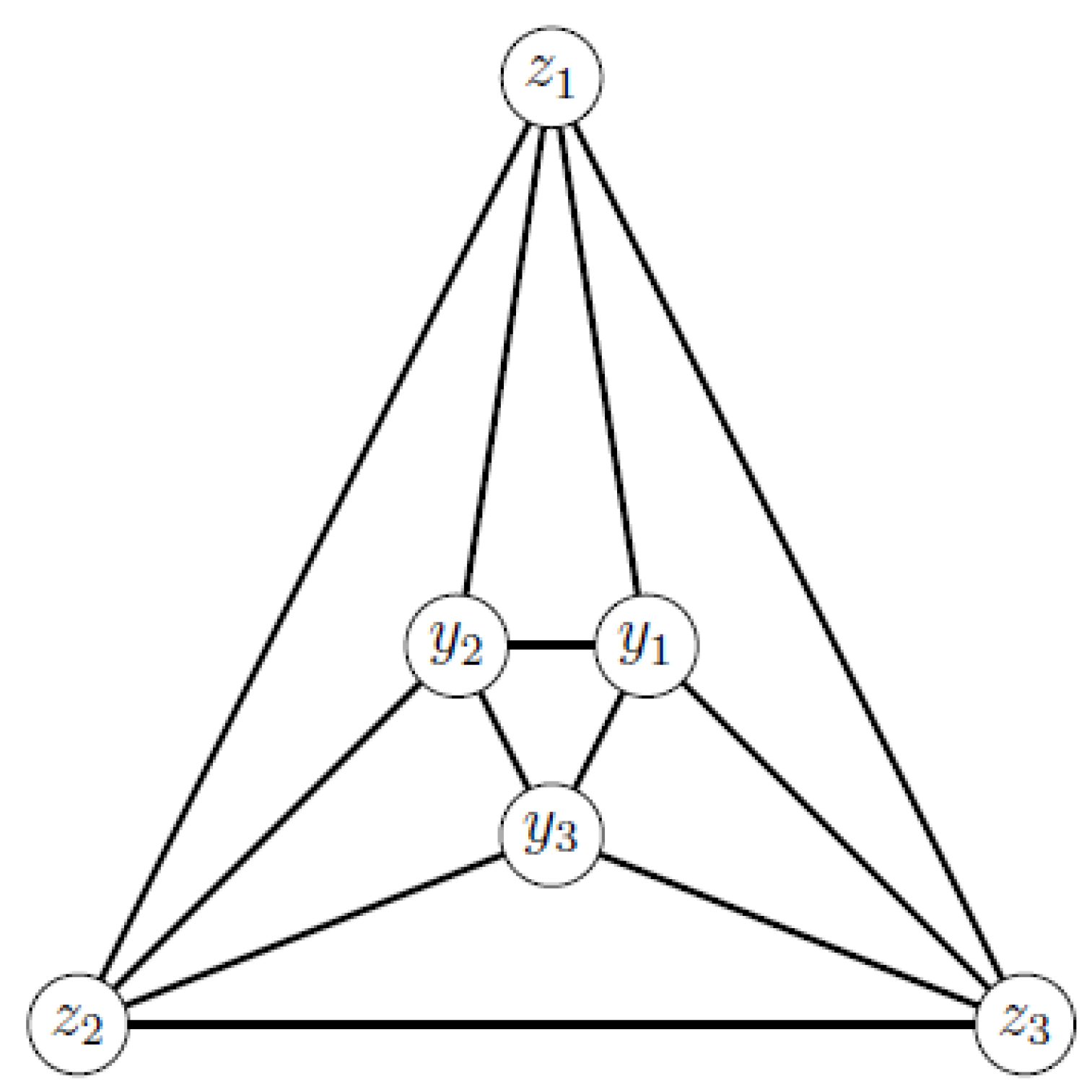
We investigate fault-tolerant resolvability in the anti-prism graphs. The anti-prism $A\left(n\right)$ [35] is a 4-regular graph. It is the octahedron for $n\ge 3$. For $n\ge 3$, the anti-prism $A\left(n\right)$ consists of an inner cycle $y_1,y_2,\dots ,y_n$, an outer cycle $z_1,z_2,\dots ,z_n$, and a set of n spokes $y_k{z}_k$ and $y_{k+1}{z}_k$, $k=1,2,\dots ,n$, with indices taken as modulo n. Thus, $\left|V\right(A\left(n\right)\left)\right|=2n$ and $\left|E\right(A\left(n\right)\left)\right|=4n$.

Javaid et al. [34] showed the following result.

Proposition 4.

[34] Let Γ be the anti-prism graph $A\left(n\right)$ with $n\ge 3$; then, $\beta \left(\mathsf{\Gamma }\right)=3$.

They also showed the following:

Proposition 5.

[34] The anti-prism graph $A\left(n\right)$ has a constant metric dimension.

In this section, we present the main results, and, for the anti-prism graph $A\left(n\right)$, the upper and lower bounds on the fault-tolerant metric dimension are proved. Note that Claim 1 in the following result was essentially shown in Proposition 4.

Theorem 10.

Let Γ be the anti-prism graph $A\left(n\right)$, with $n\ge 10$; then, $4\le {\beta }^{\prime }\left(\mathsf{\Gamma }\right)\le 14$.

Proof. 

Let $n=2\ell$ or $n=2\ell +1$ for even or odd n, respectively.

Claim 1: A resolving set R of order 3 exists in $\mathsf{\Gamma }$.

Based on the location of basis elements in G, we divide this in two cases.

Case 1: When n is even, $n=2\ell$, with $\ell \ge 3$.

For $n\ge 6$, there exists a resolving set R of cardinality 3. $R=\{z_1,z_3,z_{\ell +1}\}$ is a resolving set. Representation of the vertices in the outer cycle with respect to $\{z_1,z_3\}$ is as follows. As we can see, $C_{R\setminus \left\{z_{\ell +1}\right\}}\left(z_2\right)=(1,1)$; in general, the representations of the vertices in the outer cycle are

$$C_{R\setminus \left\{z_{\ell +1}\right\}}\left(z_k\right)=\left\{\begin{array}{cc}(k-1,k-3),\hfill & 4\le k\le \ell +1;\hfill \\ (n-k+1,k-3),\hfill & k=\ell +2,k=\ell +3;\hfill \\ (n-k+1,n-k+3),\hfill & \ell +4\le k\le n.\hfill \end{array}\right.$$

Representations of the vertices in the inner cycle are $C_{R\setminus \left\{z_{\ell +1}\right\}}\left(y_1\right)=(1,3)$, $C_{R\setminus \left\{z_{\ell +1}\right\}}\left(y_2\right)=(1,2)$, $C_{R\setminus \left\{z_{\ell +1}\right\}}\left(y_3\right)=(2,1)$. In general,

$$C_{R\setminus \left\{z_{\ell +1}\right\}}\left(y_k\right)=\left\{\begin{array}{cc}(k-1,k-3),\hfill & 4\le k\le \ell +1;\hfill \\ (\ell ,\ell -1),\hfill & k=\ell +2;\hfill \\ (\ell -1,\ell ),\hfill & k=\ell +3;\hfill \\ (n-k+2,n-k+4),\hfill & \ell +4\le k\le n.\hfill \end{array}\right.$$

Case 2: For odd n, $n=2\ell +1$ with $\ell \ge 3$. Then,

$$C_{R\setminus \left\{z_{\ell +1}\right\}}\left(y_k\right)=\left\{\begin{array}{cc}(k-1,k-3),\hfill & 4\le k\le \ell +2;\hfill \\ (\ell ,\ell ),\hfill & k=\ell +3;\hfill \\ (n-k+2,n-k+4),\hfill & \ell +4\le k\le n.\hfill \end{array}\right.$$

From the above discussion, we can see there are few vertices with the same representation $y_k$,$z_k$, with $4\le k\le \ell +1$; for even and odd n, $y_1$,$z_n$ and $y_{s+1}$,$z_s$ with $\ell +3\le s\le n-1$ and $\ell +4\le s\le n-1$, respectively. In order to distinguish the pairs with the same vertices, we take $y_{\ell +1}$ in the outer and inner cycle. Representation in the outer cycle is

$$d(y_{\ell +1},z_s)=\left\{\begin{array}{cc}\ell -s+1,\hfill & 1\le s\le \ell ;\hfill \\ s-\ell -1,\hfill & \ell +2\le s\le n.\hfill \end{array}\right.$$

Now, representation in the inner cycle is

$$d(y_{\ell +1},y_k)=\left\{\begin{array}{cc}\ell -k+2,\hfill & 1\le k\le \ell ;\hfill \\ 1,\hfill & s=\ell +1;\hfill \\ k-\ell -1,\hfill & \ell +2\le k\le \le n.\hfill \end{array}\right.$$

Also, $d(z_{\ell +1},y_1)=n-\ell$. So, from the above discussion, we see that $z_{\ell +1}$ distinguishes the vertices of $\mathsf{\Gamma }$. Hence, $R=\{z_1,z_3,z_{\ell +1}\}$ is a resolving set of $\mathsf{\Gamma }$. This shows that $\beta \left(\mathsf{\Gamma }\right)\le 3$.

Claim 2: There exists a fault-tolerant resolving set of cardinality 14 in $\mathsf{\Gamma }$.

$\mathsf{\Gamma }$ contains a resolving set R of order 3. We show that $\mathsf{\Gamma }$ has a fault-tolerant resolving set of 14. Now, we can see from Figure 4 that $N\left[z_1\right]=\{z_1,z_2,z_n,y_1,y_2\}$, $N\left[z_3\right]=\{z_2,z_3,z_4,y_3,y_4\}$, and $N\left[z_{\ell +1}\right]=\{z_{\ell },z_{\ell +1},z_{\ell +2},y_{\ell +1},y_{\ell +2}\}$. Moreover, we find that $\lambda \left(N_{\mathsf{\Gamma }}\left(z_1\right)\right)=\lambda \left(N_{\mathsf{\Gamma }}\left(z_2\right)\right)=\lambda \left(N_{\mathsf{\Gamma }}\left(z_{\ell +1}\right)\right)=\varnothing$. Thus, by using Lemma 3, we find that $R^{\prime }=\{y_1,y_2,y_3,y_4,z_1,z_2,z_3,z_4,y_{\ell +1},y_{\ell +2},z_{\ell },z_{\ell +1},z_{\ell +2},z_n\}$. Thus, there exists a fault-tolerant resolving set of $\mathsf{\Gamma }$ with cardinality 14 when $n\ge 10$.

By using Proposition 4, the above discussion, and Inequality (1), we find that ${\beta }^{\prime }\left(\mathsf{\Gamma }\right)\ge 4$. ☐

As a result of Theorem 10, we present the following corollary. It provides a fault-tolerant metric dimension analog of Proposition 5.

Corollary 2.

The anti-prism graph $A\left(n\right)$ has a constant fault-tolerant metric dimension.

Proof. 

By Theorem 10, we have $4\le {\beta }^{\prime }\left(A\left(n\right)\right)\le 14$. This implies that the fault-tolerant metric dimension of $A\left(n\right)$ does not depend on the defining parameter n. Thus, by definition, $A\left(n\right)$ is a family of graphs with a constant fault-tolerant metric dimension. ☐

In view of Lemma 3 and Proposition 4, we propose the following conjecture on the greatest lower bound on the fault-tolerant metric dimension for the anti-prism graph $A\left(n\right)$.

Conjecture 2.

Let $\mathsf{\Gamma }$ be an anti-prism graph $A\left(n\right)$ and $n\ge 10$; then, ${\beta }^{\prime }\left(\mathsf{\Gamma }\right)\ge 14$, and thus, ${\beta }^{\prime }\left(\mathsf{\Gamma }\right)=14$.

3.5. Squared Cycle Graphs

Javaid et al. [32] proved that the fault-tolerant metric dimension of cycle graphs is 3.

Lemma 4.

Let Γ be the cycle graph $C_n$, where $n\ge 3$. Then, ${\beta }^{\prime }\left(\mathsf{\Gamma }\right)=3$.

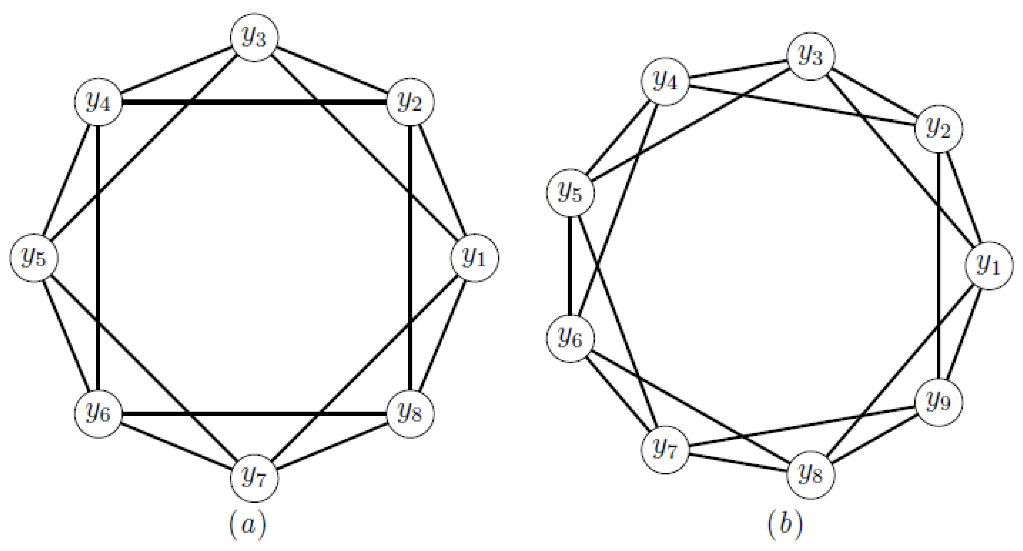
In the subsequent section, we study fault-tolerant resolvability of squared cycle graphs, which are somewhat of an extension of cycle graphs. The squared cycle graph $S\left(n\right)$ is a 4-regular graph of order n, with $V\left(S\left(n\right)\right)=\{y_1,y_2,\dots ,y_n\}$. For each $k(1\le k\le n)$, we join $y_k$ to $y_{k+1},y_{k+2}$ and to $y_{k-1},y_{k-2}$. If we cyclically arrange the vertices $y_1,y_2,\dots ,y_n$, then each vertex $y_k$ is adjacent to the 2 vertices that immediately follow $y_k$ and 2 vertices that immediately precede $y_k$. Thus, $S\left(n\right)$ is a four-regular graph. In Figure 5, we depict the squared cycle graph $S\left(n\right)$ for $n=8$ and $n=9$. Note that the squared cycle graph is a special case of the Harary graph $H(m,n)$, with $m=4$.

Javaid et al. [34] showed the following result.

Proposition 6.

[34] For $n\equiv 0,2,3(mod4)$, let Γ be the squared cycle graph $S\left(n\right)$ with $n\ge 5$. Then, $\beta \left(\mathsf{\Gamma }\right)=3$.

They also showed the following:

Proposition 7.

[34] For a positive integer n, the squared cycle graph $S\left(n\right)$ is a family of graphs with a constant metric dimension.

The following is the main result of this section. Note that Claim 1 in the following result was essentially shown in Proposition 6.

Theorem 11.

Let Γ be the squared cycle graph $S\left(n\right)$; then,

$${\beta }^{\prime }\left(\mathsf{\Gamma }\right)\le \left\{\begin{array}{cc}7,\hfill & ifn\equiv 0,2,3(mod4)withn\ge 7;\hfill \\ 12,\hfill & ifn\equiv 1(mod4)withn\ge 13,\hfill \end{array}\right.$$

and

$${\beta }^{\prime }\left(\mathsf{\Gamma }\right)\ge \left\{\begin{array}{cc}4,\hfill & ifn\equiv 0,2,3(mod4)withn\ge 5;\hfill \\ \delta ,\hfill & ifn\equiv 1(mod4)withn\ge 5.\hfill \end{array}\right.$$

where

$$\delta =\left\{\begin{array}{cc}4,\hfill & if\beta \left(\mathsf{\Gamma }\right)>2;\hfill \\ 5,\hfill & if\beta \left(\mathsf{\Gamma }\right)>3.\hfill \end{array}\right.$$

Proof. 

Let $\mathsf{\Gamma }$ be the squared cycle graph $S\left(n\right)$. We show the following claims to complete the proof.

Claim 1: There exists a resolving set R of order 3 in $\mathsf{\Gamma }$.

Case 1: When $n\equiv 0,2,3(mod4)$ with $n\ge 7$.

Based on the location of basis elements in $\mathsf{\Gamma }$, we further divide this case into three subcases.

Subcase 1.1: When $n\equiv 0(mod4)$.

We can write $n=4\ell$, $\ell \in {\mathbb{Z}}^{+}$. We prove that $R=\{y_1,y_2,y_3\}$ resolves $V\left(\mathsf{\Gamma }\right)$. In order to show that R resolves vertices of $V\left(\mathsf{\Gamma }\right)$, the representation of the vertices of $V\left(\mathsf{\Gamma }\right)$ with respect to the resolving set is given.

$$C_R\left(y_{2k}\right)=\left\{\begin{array}{cc}(k,k-1,k-1),\hfill & 2\le k\le \ell ;\hfill \\ (\ell ,\ell ,\ell ),\hfill & k=\ell +1;\hfill \\ (2\ell -k+1,2\ell -k+1,2\ell -k+2),\hfill & \ell +2\le k\le 2\ell .\hfill \end{array}\right.$$

and

$$C_R\left(y_{2k+1}\right)=\left\{\begin{array}{cc}(k,k,k-1),\hfill & 2\le k\le \ell ;\hfill \\ (2\ell -k,2\ell -k+1,2\ell -k+1),\hfill & \ell +1\le k\le 2\ell -1.\hfill \end{array}\right.$$

From the above discussion, it is shown that all vertices have a distinct representation for $n\equiv 0(mod4)$, so $\beta \left(G\right)\le 3$.

Subcase 1.2: When $n\equiv 2(mod4)$.

It can be written as $n=4\ell +2$, $\ell \in {\mathbb{Z}}^{+}$.

$$C_R\left(y_{2k}\right)=\left\{\begin{array}{cc}(k,k-1,k-1),\hfill & 2\le k\le \ell +1;\hfill \\ (2\ell -k+2,2\ell -k+2,2\ell -k+3),\hfill & \ell +2\le k\le 2\ell +1.\hfill \end{array}\right.$$

and

$$C_R\left(y_{2k+1}\right)=\left\{\begin{array}{cc}(k,k,k-1),\hfill & 2\le k\le \ell ;\hfill \\ (\ell ,\ell +1,\ell ),\hfill & k=\ell +1;\hfill \\ (2\ell -k+1,2\ell -k+2,2\ell -k+2),\hfill & \ell +2\le k\le 2\ell .\hfill \end{array}\right.$$

Again, all vertices in $\mathsf{\Gamma }$ have a distinct representation, which shows that $\beta \left(\mathsf{\Gamma }\right)\le 3$ when $n\equiv 2(mod4)$.

Subcase 1.3: When $n\equiv 3(mod4)$.

We can write $n=4\ell +3$, $\ell \in {\mathbb{Z}}^{+}$.

$$C_R\left(y_{2k}\right)=\left\{\begin{array}{cc}(k,k-1,k-1),\hfill & 2\le k\le \ell +1;\hfill \\ (2\ell -k+2,2\ell -k+3,2\ell -k+3),\hfill & \ell +2\le k\le 2\ell +1.\hfill \end{array}\right.$$

and

$$C_R\left(y_{2k+1}\right)=\left\{\begin{array}{cc}(k,k,k-1),\hfill & 2\le k\le \ell +1;\hfill \\ (2\ell -k+2,2\ell -k+2,2\ell -k+3),\hfill & \ell +2\le k\le 2\ell +1.\hfill \end{array}\right.$$

Once again, we can see that all vertices in $\mathsf{\Gamma }$ have a distinct representation, which shows that $\beta \left(\mathsf{\Gamma }\right)\le 3$ when $n\equiv 3(mod4)$.

Claim 2:$\mathsf{\Gamma }$ has a fault-tolerant resolving set of cardinality 7 when $n\ge 7$.

We can write $n=4\ell$, $\ell \ge 2$, $\ell \in {\mathbb{Z}}^{+}$. Note that, in this case, $R=\{y_1,y_2,y_3\}$ is a resolving set of $\mathsf{\Gamma }$. We show that $\mathsf{\Gamma }$ is the graph in which there exists a fault-tolerant resolving set of cardinality 7. From Figure 5, it can be observed that $N\left[y_1\right]=\{y_1,y_2,y_3,y_{n-1},y_n\}$, $N\left[y_2\right]=\{y_1,y_2,y_3,y_4,y_n\}$, and $N\left[y_3\right]=\{y_1,y_2,y_3,y_4,y_5\}$. Moreover, we find that $\lambda \left(N_{\mathsf{\Gamma }}\left(y_1\right)\right)=\lambda \left(N_{\mathsf{\Gamma }}\left(y_2\right)\right)=\lambda \left(N_{\mathsf{\Gamma }}\left(y_3\right)\right)=\varnothing$. Thus, by using Lemma 3, we find that $R^{\prime }=\{y_1,y_2,y_3,y_4,y_5,y_{n-1},y_n\}$ is a fault-tolerant resolving set of $\mathsf{\Gamma }$. Thus, it is shown that a fault-tolerant resolving set of $\mathsf{\Gamma }$ with cardinality 7 exists when $n\ge 7$.

Claim 1: There exists a resolving set R of order 4 in $\mathsf{\Gamma }$.

Case 1: When $n\equiv 1(mod4)$.

Now, we can write $n=4\ell +1$, $\ell \in {\mathbb{Z}}^{+}$.

$$C_R\left(y_{2k}\right)=\left\{\begin{array}{cc}(k,k-1,k-1),\hfill & 2\le k\le \ell ;\hfill \\ (\ell ,\ell ,\ell ),\hfill & k=\ell +1;\hfill \\ (2\ell -k+1,2\ell -k+2,2\ell -k+2),\hfill & \ell +2\le k\le 2\ell .\hfill \end{array}\right.$$

and

$$C_R\left(y_{2k+1}\right)=\left\{\begin{array}{cc}(k,k,k-1),\hfill & 2\le k\le \ell ;\hfill \\ (\ell ,\ell ,\ell ),\hfill & k=\ell +1;\hfill \\ (2\ell -k+1,2\ell -k+1,2\ell -k+2),\hfill & \ell +2\le k\le 2\ell .\hfill \end{array}\right.$$

For $n\equiv 1(mod4)$, the vertices $y_{2\ell +2}$ and $y_{2\ell +3}$ have the same representation. In order to have distinct representations, we add $y_{2\ell +2}$ to the resolving set R. Now, $R^{\prime }=\{y_1,y_2,y_3,y_{2\ell +2}\}$ resolves $V\left(\mathsf{\Gamma }\right)$. So, it is shown that $\beta \left(\mathsf{\Gamma }\right)\le 4$ for $n\equiv 1(mod4)$.

Claim 2: When $n\ge 13$, $\mathsf{\Gamma }$ has a fault-tolerant resolving set of cardinality 12. It can be written $n=4\ell +1$, $\ell \ge 3$, $\ell \in {\mathbb{Z}}^{+}$. Now, for this, $R=\{y_1,y_2,y_3,y_{2\ell +2}\}$ is a resolving set of $\mathsf{\Gamma }$. We show that $\mathsf{\Gamma }$ has a fault-tolerant resolving set of cardinality 12. From Figure 5, it can be observed that $N\left[y_1\right]=\{y_1,y_2,y_3,y_{n-1},y_n\}$, $N\left[y_2\right]=\{y_1,y_2,y_3,y_4,y_n\}$, $N\left[y_3\right]=\{y_1,y_2,y_3,y_4,y_5\}$, and $N\left[y_{2\ell +2}\right]=\{y_{2\ell },y_{2\ell +1},y_{2\ell +2},y_{2\ell +3},y_{2\ell +4}\}$. Moreover, we find that $\lambda \left(N_{\mathsf{\Gamma }}\left(y_1\right)\right)=\lambda \left(N_{\mathsf{\Gamma }}\left(y_2\right)\right)=\lambda \left(N_{\mathsf{\Gamma }}\left(y_3\right)\right)=\lambda \left(N_{\mathsf{\Gamma }}\left(y_{2\ell +2}\right)\right)=\varnothing$. Thus, by using Lemma 3, we find that $R^{\prime }=\{y_1,y_2,y_3,y_4,y_5,y_{n-1},y_n,y_{2\ell },y_{2\ell +1},y_{2\ell +2},y_{2\ell +3},y_{2\ell +4}\}$ is a fault-tolerant resolving set of $\mathsf{\Gamma }$. Thus, $\mathsf{\Gamma }$ is the graph in which there exists a fault-tolerant resolving set of cardinality 12 when $n\ge 13$. In view of Lemma 3 and Proposition 1, we find enough reasoning to propose the following conjecture on the lower bound of the fault-tolerant metric dimension for the squared cycle graph $S\left(n\right)$.

From the above discussion, Inequality, and Proposition 6, we find that

$${\beta }^{\prime }\left(\mathsf{\Gamma }\right)\ge \left\{\begin{array}{cc}4,\hfill & ifn\equiv 0,2,3(mod4)withn\ge 5;\hfill \\ \delta ,\hfill & ifn\equiv 1(mod4)withn\ge 5.\hfill \end{array}\right.$$

where

$$\delta =\left\{\begin{array}{cc}4,\hfill & if\beta \left(\mathsf{\Gamma }\right)>2;\hfill \\ 5,\hfill & if\beta \left(\mathsf{\Gamma }\right)>3.\hfill \end{array}\right.$$

 ☐

Because of Theorem 11, the following corollary is presented. It provides a fault-tolerant metric dimension analogous to Proposition 7.

Corollary 3.

The squared cycle graph $S\left(n\right)$ is a family of graphs with a constant fault-tolerant metric dimension.

Proof. 

By Theorem 11, we have

$${\beta }^{\prime }\left(S\left(n\right)\right)\le \left\{\begin{array}{cc}7,\hfill & ifn\equiv 0,2,3(mod4)withn\ge 7;\hfill \\ 12,\hfill & ifn\equiv 1(mod4)withn\ge 13,\hfill \end{array}\right.$$

and

$${\beta }^{\prime }\left(\mathsf{\Gamma }\right)\ge \left\{\begin{array}{cc}4,\hfill & ifn\equiv 0,2,3(mod4)withn\ge 5;\hfill \\ \delta ,\hfill & ifn\equiv 1(mod4)withn\ge 5.\hfill \end{array}\right.$$

where

$$\delta =\left\{\begin{array}{cc}4,\hfill & if\beta \left(\mathsf{\Gamma }\right)>2;\hfill \\ 5,\hfill & if\beta \left(\mathsf{\Gamma }\right)>3.\hfill \end{array}\right.$$

This implies that the fault-tolerant metric dimension of $S\left(n\right)$ does not depend on the defining parameter n. Thus, by definition, $S\left(n\right)$ is a family of graphs with a constant fault-tolerant metric dimension. ☐

In view of Lemma 3 and Proposition 6, the following conjecture is proposed.

Conjecture 3.

Let $\mathsf{\Gamma }$ be the squared cycle graph $S\left(n\right)$ such that $n\equiv 0,2,3(mod4)$, with $n\ge 7$. Then, ${\beta }^{\prime }\left(\mathsf{\Gamma }\right)\ge 7$; thus, we have ${\beta }^{\prime }\left(\mathsf{\Gamma }\right)=7$.

4. Concluding Remarks

This paper investigates the fault-tolerant metric dimension of graphs. We present certain characterizations of graphs with some extreme values of the fault-tolerant metric dimension. A method is presented to calculate the upper bounds on the fault-tolerant metric dimension of graphs. We study fault-tolerant resolvability in three non-finite families of regular graphs and show that they are the families of graphs with a constant fault-tolerant metric dimension. The following remark shows a comparison between the upper bound produced by our method and the upper bound by Hernando et al.

Remark 1.

Note that the upper bound on the fault-tolerant metric dimension provided by Theorem 4 is always crude. For example, if $\mathsf{\Gamma }\in \left\{P\right(n),A(n\left)\right\}$ or $S\left(n\right)$, with $n\equiv 0,2,3(mod4)$, then by using $\beta \left(\mathsf{\Gamma }\right)=3$ in Theorem 4, we obtain ${\beta }^{\prime }\left(\mathsf{\Gamma }\right)\le 153$, which is not interesting. In view of this fact, Lemma 3 always gives a much better bound on ${\beta }^{\prime }\left(\mathsf{\Gamma }\right)$.

Recently, Raza et al. [36] studied the fault-tolerant metric dimension of hexagonal, honeycomb, and hex-derived networks. See [37] for a study of hexagonal and honeycomb networks. We conclude the paper with some open problems.

Problem 1.

In view of the characterizations of graphs with fault-tolerant metric dimension 2 and $n-1$, the following open problems are proposed.

(i)

Characterize n-ordered graphs with fault-tolerant metric dimension 3.

(ii)

Characterize n-ordered graphs with fault-tolerant metric dimension $n-2$.

We also propose the following open problems:

(i)

Study the fault-tolerant metric dimension of other interesting families of the regular graph, such as the prism graphs, and the generalized Petersen graphs $P(n,m)$, $m>2$.

(ii)

Investigate the fault-tolerant metric dimension of strongly regular graphs, such as the square grid graphs and the triangular graphs.

(iii)

In view of Raza et al. [36], study the fault-tolerant resolvability in other direct and multiplex interconnection networks, such as the butterfly and Benes networks.

(iv)

Study the applicability of fault-tolerant resolvability in the optimal flow control of multiplex interconnection networks; see, for example, [38,39,40] for a through study on multiplex networks.

References

- Slater, P.J. Leaves of trees. Proceedings of the 6th Southeastern Conference on Combinatorics, Graph Theory, and Computing. Congr. Numer. 1975, 14, 549–559. [Google Scholar]
- Harary, F.; Melter, R.A. On the metric dimension of a graph. Ars Comb. 1976, 2, 191–195. [Google Scholar]
- Khuller, S.; Raghavachari, B.; Rosenfeld, A. Landmarks in graphs. Discret. Appl. Math. 1996, 70, 217–229. [Google Scholar] [CrossRef] [Green Version]
- Liu, K.; Abu-Ghazaleh, N. Virtual coordinate back tracking for void travarsal in geographic routing. Lect. Notes Comput. Sci. 2006, 4104, 46–59. [Google Scholar]
- Beerloiva, Z.; Eberhard, F.; Erlebach, T.; Hall, A.; Hoffmann, M.; Mihalák, M.; Ram, L. Network discovery and verification. IEEEE J. Sel. Area Commun. 2006, 24, 2168–2181. [Google Scholar] [CrossRef]
- Chartrand, G.; Eroh, L.; Johnson, M.A.; Oellermann, O.R. Resolvability in graphs and the metric dimension of a graph. Discret. Appl. Math. 2000, 150, 99–113. [Google Scholar] [CrossRef]
- Bailey, R.F.; Meagher, K. On the metric dimension of Grassmann graphs. Discret. Math. Theor. Comput. Sci. 2011, 13, 97–104. [Google Scholar]
- Bailey, R.F.; Cameron, P.J. Basie size, metric dimension and other invariants of groups and graphs. Bull. Lond. Math. Soc. 2011, 43, 209–242. [Google Scholar] [CrossRef]
- Fehr, M.; Gosselin, S.; Oellermann, O. The metric dimension of Cayley digraphs. Discret. Math. 2006, 306, 31–41. [Google Scholar] [CrossRef] [Green Version]
- Ahmad, A.; Imran, M.; Al-Mushayt, O.; Bokhary, S.A.U.H. On the metric dimension of barycentric subdividion of Cayley graph Cay(Zn⊕Zm). Miskolc Math. Notes 2015, 16, 637–646. [Google Scholar]
- Cáceres, J.; Hernando, C.; Mora, M.; Pelayoe, I.M.; Puertas, M.L.; Seara, C.; Wood, D.R. On the metric dimension of cartesian products of graphs. SIAM J. Discret. Math. 2007, 21, 423–441. [Google Scholar] [CrossRef]
- Vetrík, T.; Ahmad, A. Computing the metric dimension of the categorial product of some graphs. Int. J. Comput. Math. 2015, 94, 363–371. [Google Scholar] [CrossRef]
- Siddiqui, H.M.A.; Imran, M. Computing the metric dimension of wheel related graphs. Appl. Math. Comput. 2014, 242, 624–632. [Google Scholar]
- Kratica, J.; Kovačević-Vujčić, V.; Čangalović, M.; Stojanović, M. Minimal doubly resolving sets and the strong metric dimension of some convex polytopes. Appl. Math. Comput. 2012, 218, 9790–9801. [Google Scholar] [CrossRef]
- Imran, M.; Siddiqui, H.M.A. Computing the metric dimension of conves polytopes generated by the wheel related graphs. Acta Math. Hung. 2016, 149, 10–30. [Google Scholar] [CrossRef]
- Cáceres, J.; Hernando, C.; Mora, M.; Pelayoe, I.M.; Puertas, M.L. On the metric dimension of infinite graphs. Electron. Notes Discret. Math. 2009, 35, 15–20. [Google Scholar] [CrossRef]
- Garey, M.R.; Johnson, D.S. Computers and Intractability: A Guide to the Theory of NP–Completeness; W.H. Freeman and Company: New York, NY, USA, 1979. [Google Scholar]
- Hernando, C.; Mora, M.; Slater, P.J.; Wood, D.R. Fault-tolerant metric dimension of graphs. In Proceedings International Conference on Convexity in Discrete Structures; Ramanujan Mathematical Society Lecture Notes; Ramanujan Mathematical Society: Tiruchirappalli, India, 2008; pp. 81–85. [Google Scholar]
- Chartrand, G.; Zhang, P. The theory and applications of resolvability in graphs: A survey. Congr. Numer. 2003, 160, 47–68. [Google Scholar]
- Krishnan, S.; Rajan, B. Fault-tolerant resolvability of certain crystal structures. Appl. Math. 2016, 7, 599–604. [Google Scholar] [CrossRef]
- Raza, H.; Hayat, S.; Pan, X.-F. On the fault-tolerant metric dimension of convex polytopes. Appl. Math. Comput. 2018, 339, 172–185. [Google Scholar] [CrossRef]
- Raza, H.; Hayat, S.; Pan, X.-F. Binary locating-dominating sets in rotationally-symmetric convex polytopes. Symmetry 2018, 10, 727. [Google Scholar] [CrossRef]
- Salman, M.; Javaid, I.; Chaudhry, M.A. Minimum fault-tolerant, local and strong metric dimension of graphs. arXiv, 2014; arXiv:1409.2695. [Google Scholar]
- Hayat, S. Computing distance-based topological descriptors of complex chemical networks: New theoretical techniques. Chem. Phys. Lett. 2017, 688, 51–58. [Google Scholar] [CrossRef]
- Hayat, S.; Imran, M. Computation of topological indices of certain networks. Appl. Math. Comput. 2014, 240, 213–228. [Google Scholar] [CrossRef]
- Hayat, S.; Malik, M.A.; Imran, M. Computing topological indices of honeycomb derived networks. Rom. J. Inf. Sci. Technol. 2015, 18, 144–165. [Google Scholar]
- Hayat, S.; Wang, S.; Liu, J.-B. Valency-based topological descriptors of chemical networks and their applications. Appl. Math. Model. 2018, 60, 164–178. [Google Scholar] [CrossRef]
- Imran, M.; Hayat, S.; Malik, M.Y.H. On topological indices of certain interconnection networks. Appl. Math. Comput. 2014, 244, 936–951. [Google Scholar] [CrossRef]
- Bondy, J.A.; Murty, U.S.R. Graph Theory; Springer: New York, NY, USA, 2008. [Google Scholar]
- Shang, Y. Resilient consensus of switched multi-agent systems. Syst. Control Lett. 2018, 122, 12–18. [Google Scholar] [CrossRef]
- Shang, Y. Resilient multiscale coordination control against adversarial nodes. Energies 2018, 11, 1844. [Google Scholar] [CrossRef]
- Javaid, I.; Salman, M.; Chaudhry, M.A.; Shokat, S. Fault-tolerance in resolvibility. Util. Math. 2009, 80, 263–275. [Google Scholar]
- Watkins, M.E. A theorem on Tait colorings with an application to the generalized Petersen graphs. J. Comb. Theory 1969, 6, 152–164. [Google Scholar] [CrossRef]
- Javaid, I.; Rahim, T.; Ali, K. Families of regular graphs with constant metric dimension. Util. Math. 2008, 65, 21–33. [Google Scholar]
- Gallian, J.A. A dynamic survey of graph labeling. Electron. J. Comb. 2018, #DS6, 1–219. [Google Scholar] [PubMed]
- Raza, H.; Hayat, S.; Pan, X.-F. On the fault-tolerant metric dimension of certain interconnection networks. J. Appl. Math. Comput. 2018. [Google Scholar] [CrossRef]
- Chen, M.S.; Shin, K.G.; Kandlur, D.D. Addressing, routing and broadcasting in hexagonal mesh multiprocessors. IEEE Trans. Comput. 1990, 39, 10–18. [Google Scholar] [CrossRef]
- Wang, W.-H.; Palaniswami, M.; Low, H.L. Optimal flow control and routing in multi-path networks. Perform. Eval. 2003, 52, 119–132. [Google Scholar] [CrossRef]
- Shang, Y. Deffuant model of opinion formation in one-dimensional multiplex networks. J. Phys. A Math. Theor. 2015, 48, 395101. [Google Scholar] [CrossRef]
- Antonopoulos, C.G.; Shang, Y. Opinion formation in multiplex networks with general initial distributions. Sci. Rep. 2018, 8, 2852. [Google Scholar] [CrossRef]
Figure 1.
The tree example from Hernando et al. [18].
Figure 2.
A depiction of the proof of Lemma 3.
Figure 3.
(a) The extended Petersen graph , (b) The extended Petersen graph .
Figure 4.
The anti-prism graph .
Figure 5.
(a) The squared cycle graph , (b) the squared cycle graph .
© 2019 by the authors. Licensee MDPI, Basel, Switzerland. This article is an open access article distributed under the terms and conditions of the Creative Commons Attribution (CC BY) license (http://creativecommons.org/licenses/by/4.0/).
Share and Cite
MDPI and ACS Style
Raza, H.; Hayat, S.; Imran, M.; Pan, X.-F. Fault-Tolerant Resolvability and Extremal Structures of Graphs. Mathematics 2019, 7, 78. https://doi.org/10.3390/math7010078
AMA Style
Raza H, Hayat S, Imran M, Pan X-F. Fault-Tolerant Resolvability and Extremal Structures of Graphs. Mathematics. 2019; 7(1):78. https://doi.org/10.3390/math7010078
Chicago/Turabian StyleRaza, Hassan, Sakander Hayat, Muhammad Imran, and Xiang-Feng Pan. 2019. "Fault-Tolerant Resolvability and Extremal Structures of Graphs" Mathematics 7, no. 1: 78. https://doi.org/10.3390/math7010078
Note that from the first issue of 2016, this journal uses article numbers instead of page numbers. See further details here.