Image Interpolation Using a Rational Bi-Cubic Ball
by
 , and
, and
Nur Atiqah Binti Zulkifli
1, 
Samsul Ariffin Abdul Karim
2,*,
A’fza Binti Shafie
1,
Muhammad Sarfraz
3,
Abdul Ghaffar
4 and
and
Kottakkaran Sooppy Nisar
5,*
1
Fundamental and Applied Sciences Department, Universiti Teknologi PETRONAS, Bandar Seri Iskandar, Seri Iskandar 32610, Perak DR, Malaysia
2
Fundamental and Applied Sciences Department and Centre for Smart Grid Energy Research (CSMER), Institute of Autonomous System, Universiti Teknologi PETRONAS, Bandar Seri Iskandar, Seri Iskandar 32610, Perak DR, Malaysia
3
Department of Information Science, College of Computing Sciences & Engineering, Kuwait University, P.O. Box # 5969, Safat 13060, Kuwait
4
Department of Mathematical Sciences, BUITEMS, Quetta 87300, Pakistan
5
Department of Mathematics, College of Arts and Sciences, Prince Sattam bin Abdulaziz University, Wadi Aldawaser 11991, Saudi Arabia
*
Authors to whom correspondence should be addressed.
Mathematics 2019, 7(11), 1045; https://doi.org/10.3390/math7111045
Submission received: 21 August 2019
/
Revised: 8 September 2019
/
Accepted: 11 September 2019
/
Published: 3 November 2019
(This article belongs to the Special Issue Mathematical Modeling and Simulation in Science and Engineering Education)
Abstract
:This study deals with the application of new rational bi-cubic Ball function with six parameters in image interpolation, especially for the grayscale image. These six free parameters can be modified to get better and quality image resolution, and refine the shape of the interpolating surface. This bivariate rational Ball function has been extended from univariate cases by using a tensor product approach. The proposed scheme is tested for image upscaling with factors of two and four through an efficient algorithm. The effectiveness of the proposed scheme is measured by using an image quality assessment (IQA), such as peak-signal-to-noise-ratio (PSNR), root mean square error (RMSE) or feature similarity (FSIM) index. Numerical and graphical results with comparisons against some existing scheme are presented by using MATLAB. The proposed scheme resulted in higher PSNR and FSIM, and smaller RMSE. Thus, the new rational bi-cubic Ball with six parameters is better than the existing scheme via an efficient algorithm.
1. Introduction
Image scaling (up/down) is the task of resizing a digital image, that requires an image interpolation to obtain better resolution. Image interpolation is important in digital signal and image processing [1]. It is a tool that is widely used in image processing tasks, such as zooming, shrinking, rotating and for geometric corrections [2]. In fact, the technology of image processing is widely implemented in many areas such as medical, geology and forensic. There are numerous studies related to image processing and image interpolation due to its benefit to the industry. The technology of digital image processing appeared in the early 1960s through the introduction of the first computer. The moon is the first image taken by Ranger 7 on 31 July 1964 that was used for geometric correction [2]. From then until present, this topic has grown vigorously and lead multifarious research areas.
The common method for image interpolation is bi-cubic spline interpolation that is well documented in MATLAB as interp2 and imresize built-in functions [1]. However, bi-cubic spline requires more computational cost and memory compared to cubic spline. However, for many images, bi-cubic spline gives a higher peak signal-to-noise ratio (PSNR) and root mean square error (RMSE) value. Without a free parameter in the spline description, the user cannot alter the surfaces and images. To overcome this issue, many researchers have suggested various types of rational spline, such as the rational quartic spline, a rational cubic spline with a linear denominator and a rational cubic spline with a quadratic denominator [3,4,5,6,7,8,9] However, these methods suffer from the fact that some of them require the modification of the first partial derivative [3,4,5,6,7]. Researchers in [3,4,7,8] only consider true function value, i.e., where the first derivative is not supplied, and use only, at most, two parameters [10,11].
In early 1974, Ball introduced the main usage of the function to design a Boeing fuselage, as it has the capability to produce a conic section [12]. Majeed et al. [13] have investigated the application of a rational cubic Ball with two parameters for craniofacial reconstruction by utilizing the rational cubic Ball (curve) and reconstructing the curve of the images after doing the image detection to the outer part of the given images [14]. The proposed scheme will be used for image interpolation; i.e., image upscaling through an efficient algorithm. For example, if the original image has a size of about 256 × 256 pixels, then the image output is upgraded by a factor of two; i.e., 512 × 512 pixels. This is an effective topic in image processing, with recent challenges being to find the best function for upscaling images to specific needs, such as PSNR, RMSE and a feature similarity (FSIM) index. Table 1 and Table 2 show works of the existing scheme. Table 3 shows the list of abbreviations used in this study.
Since the scheme with more free parameters gives the better quality of image interpolation (upscaling or downscaling), it motivated us to present a new rational bi-cubic Ball function with six parameters defined on rectangular meshes. The main objectives of study are stated as follows:
- (a)
- To propose a new rational bi-cubic Ball with six parameters.
- (b)
- To apply the proposed scheme in the application of image interpolation: image upscaling for grayscale images.
- (c)
- To compare the performance with the existing schemes, such as bi-cubic spline interpolation, nearest neighbor, bilinear interpolant and Karim and Saaban [11].
The remainder of this paper is structured as follows. Section 2 deals with construction of a bivariate rational Ball function with six parameters. The relevant research methodology is described in Section 3. The results and discussion are given in Section 4, while Section 5 is devoted to the conclusion.
2. Rational Bicubic Ball Function
This section discusses the construction of a bivariate rational Ball function with six parameters, which is actually the extension of a univariate rational Ball [18] by adopting tensor product technique.
2.1. A Rational Cubic Ball with Three Parameters
The data set is given, where with the first derivative . Let, , and , . On each subinterval , . Thus, the rational cubic Ball interpolant with three parameters, and , is defined as follows
where,
The rational function satisfies continuity as follows:
when ; then and ; then,
Thus, the rational cubic Ball defined in Equation (1) can be written as:
2.2. A Rational Bi-Cubic Ball with Six Parameters
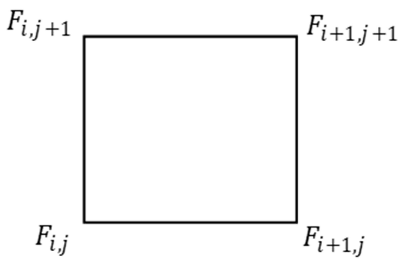
The univariate Ball given in Equation (1) is extended to the bivariate case by adopting a similar approach to [11]. The rational bi-cubic functions over each rectangular patch , where and , with the first partial derivative at the starting point, on -direction, -direction (see Figure 1), and the mixed partial derivative with respective , , and . Let, , , and and , with and . Thus, the rational bi-cubic Ball with six parameters addressed as , , , , , , and , which is defined as below:
with
where,
After some mathematical derivation, the proposed rational bi-cubic Ball surface satisfies Equation (6) below:
Based on the observation towards the image refinement when the value of six free parameters in the description were being modified, the proposed rational bi-cubic Ball in Equation (5) can be reduced to a standard bi-cubic Hermite interpolation, where , , , and , .
3. Application in Image Processing
In this section, an efficient algorithm to apply the proposed scheme into application grayscale image upscaling with factors two and four is introduced. The algorithm is comprised of several steps which are elaborated in a flowchart, as shown in Figure 2.
3.1. An Efficient Algorithm for Image Upscaling Using a Rational Bi-Cubic Ball
An efficient algorithm was constructed to implement the proposed scheme in application of image interpolation with grayscale image upscaling. This algorithm requires an input image and parametric values to start the first step. The size of image in pixels can be read as corresponding to vector form that refers to the pixel points that would be interpolated. Figure 2 displays the steps of image (up/down) scaling for factors with even numbers.
3.2. Image Quality Assessment
Image quality assessment (IQA) is used to perceive the quality of the image in many terms, such as peak-signal-to-noise-ratio (PSNR), root mean square error (RMSE) or feature similarity (FSIM) index. In addition, the standard mean square error (MSE) does not have the capability of the human visual system (HVS), to understand an image mainly according to its low-level features [19]. Table 4 provides the lists of terminologies and symbols used in Equations (7)–(9).
The value of PSNR, RMSE and FSIM is defined as follows:
- (a)
- Peak signal-to-noise ratio (PSNR)where,
- (b)
- Root mean square error (RMSE)
- (c)
- Feature similarity (FSIM) index on the domainwhere,with
3.3. Parameter Selection
The parametric values are required as inputs to run the proposed function that is used to interpolate the tested image. The parameter selection was done by simulation using MATLAB software version 2015 on version on an Intel® Core™ i5-8250U 1.60 GHz. The stopping criteria used was a PSNR value. If the PSNR value is higher, then the scheme gives a better interpolation image [1]. Figure 3 below shows the steps of parameter simulation:
The parametric values for , , , , and are varied from lowest value, 0.1, to the highest (optimum value) until the highest PSNR is reached. The list of parameters with different values for the image of “fishing boat” are explained in Table 5, where P1–P27 are the parametric values, and the impact of the parameter set towards PSNR is illustrated graphically in Figure 4 and Figure 5. Based on the Figure 4 and Figure 5, the highest PSNR value obtained among the parameter set (P1–P27) is P10, with values 39.80 and 38.02 for the factors 2 and 4, respectively. Hence, parameter set P10 is used as reference to alter the value of each parameters as shown in Table 6. Table 7 displays the list of parametric values that used in proposed function for all tested images for image upscaling with the factors two and four respectively.
4. Result and Discussion
In this section, the proposed rational bi-cubic Ball image interpolation scheme as defined in Equation (5) is tested and compared with some existing scheme. Ten tested grayscale images with size pixels were chosen, and are shown in Figure 6. The tested images were done with sampling with factors two or four first, to get low-resolution which later one re-upscale with the same factor using the proposed rational bi-cubic Ball function.
The comparison results in terms of PSNR, RMSE and FSIM between the proposed scheme and others are denoted BB. Some existing schemes, such as the conventional method for interpolation are denoted as follows: nearest neighbor (NN), bilinear (BL) and bi-cubic spline (BC), bi-cubic Hermite (BH) and Karim and Saaban [11] (KS). They are shown in Table 8, Table 9 and Table 10. Concerning overall results, we have concluded the proposed scheme gives better results for almost all images, as highlighted in the Table 8, Table 9 and Table 10, compared to existing schemes for various types of IQA used in this study.
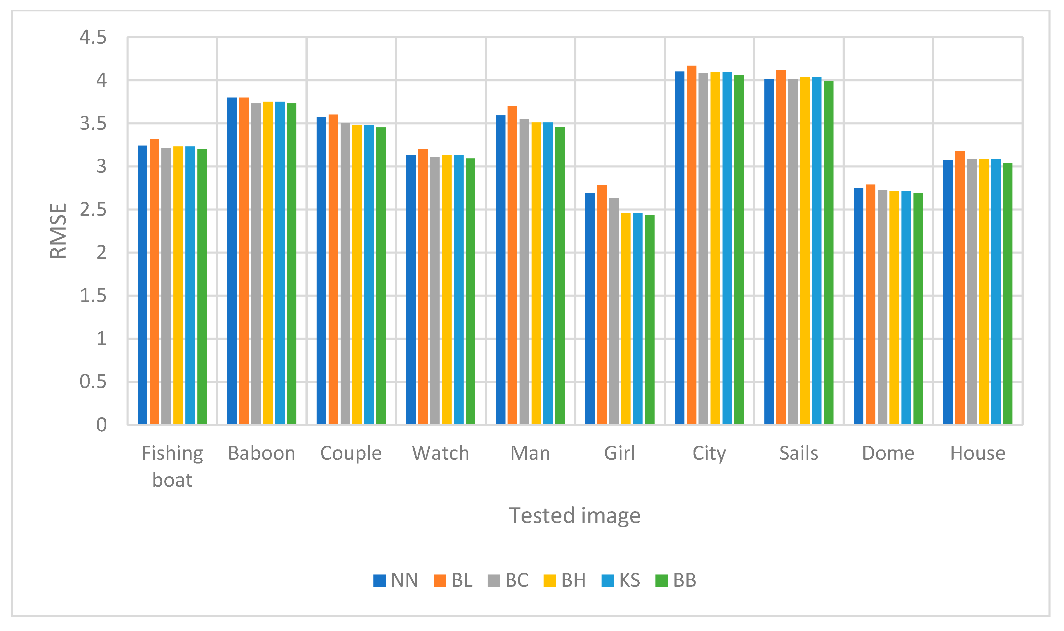
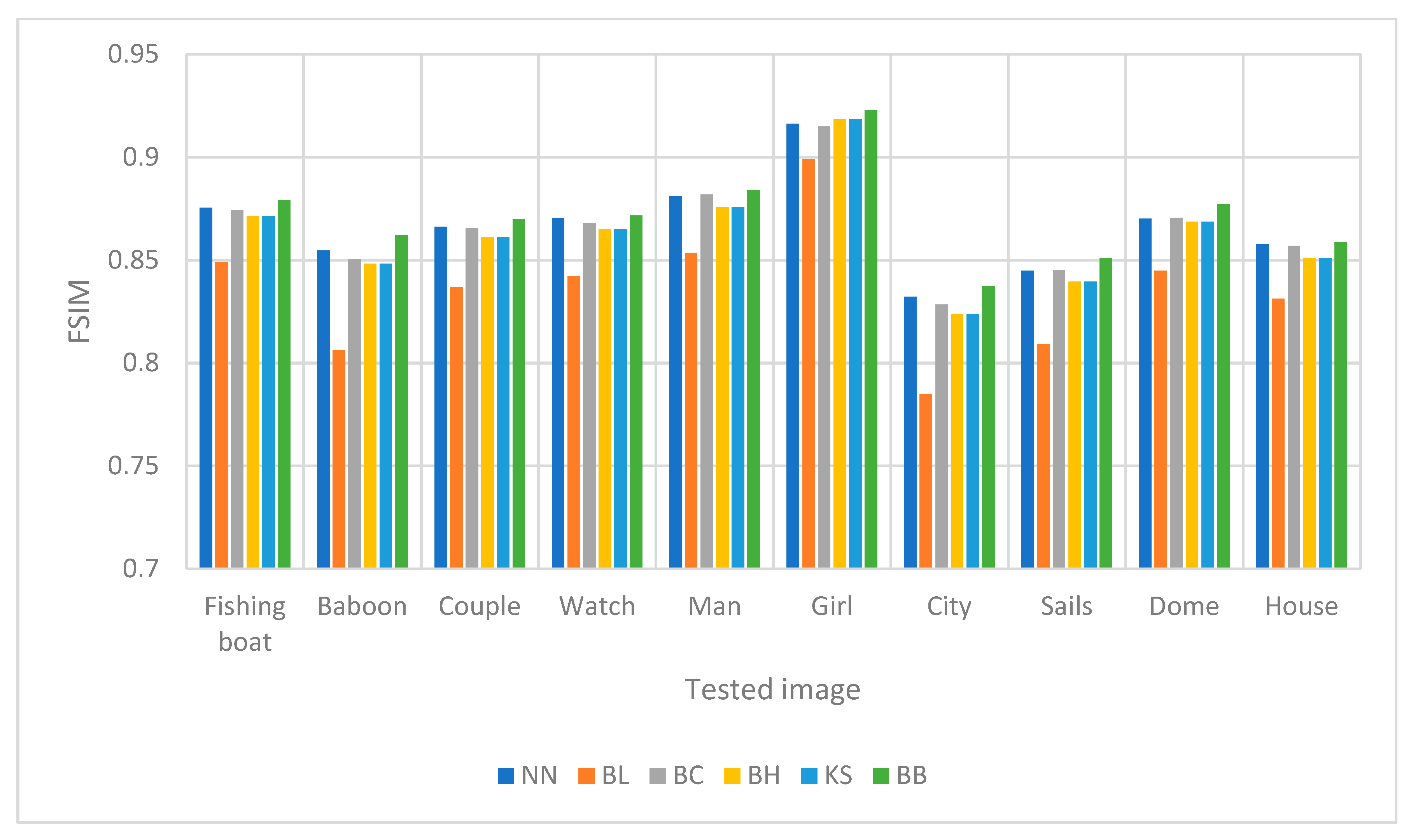
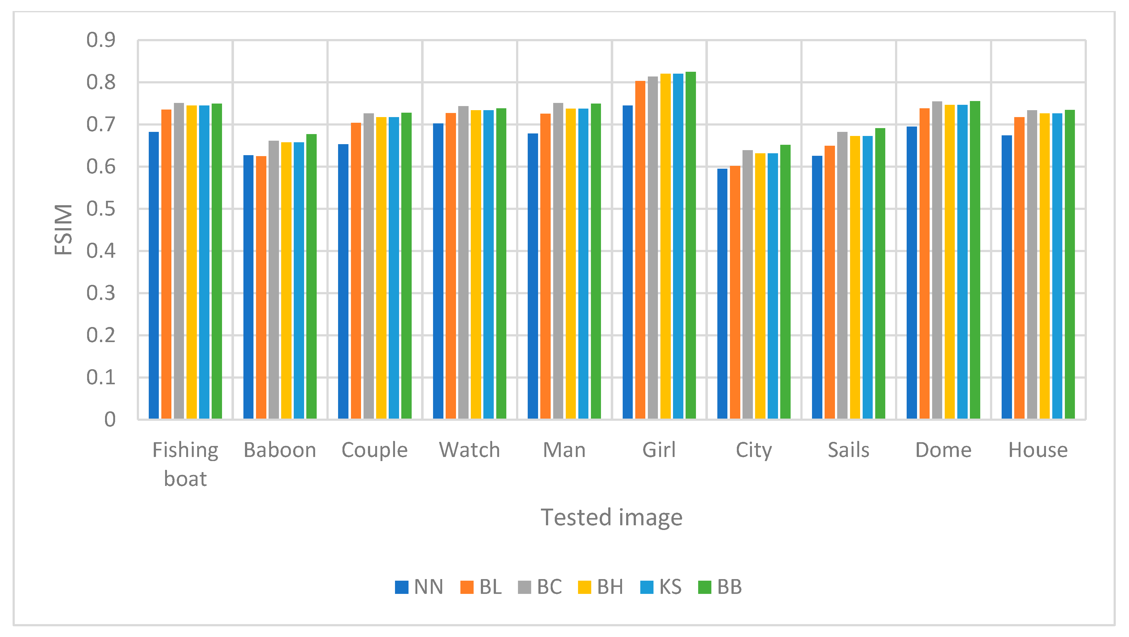
Figure 7 and Figure 8 show the comparison of PSNR values between image upscaling with factors two and four. Meanwhile, Figure 9 and Figure 10, show the bar charts for the RMSE values for factors two and four, respectively. Figure 11 and Figure 12, show the FSIM values for image upscaling with factors two and four, respectively. Figure 7, Figure 8, Figure 9, Figure 10, Figure 11 and Figure 12 were obtained by using the information gathered in Table 8, Table 9 and Table 10.
From the numerical experiments by using ten different grayscale images, we found that the proposed scheme, i.e., the rational bi-cubic Ball function, gave higher PSNR values for all images compared with well-established schemes; i.e., bilinear, nearest neighbor, bi-cubic Hermite spline, bi-cubic spline and Karim and Saaban [11]. Image upscaling with a factor of two gave higher PSNR values compared with image upscaling with a factor of four. The main reason is that, to upscale the image four times, then the size of the images will be four times larger than the original image. This will result the low quality, to an extent, in the upscaled images. But the results still better than the other five schemes. In term of FSIM, we found that for all images the proposed scheme is better than the other schemes, as can be seen in Table 10. Finally, in terms of RMSE, we found that the proposed scheme gave smaller value for most images. The results were obtained by simulation to find the best parametric values that would give the best results. This can be considered a new finding, since in [11] there were no free parameters to refine the image interpolation.
5. Conclusions
The numerical comparison of the rational bi-cubic Ball with the existing schemes has been done in detail, and the results show that the proposed scheme gives comparable results, with some advantages. Based on Figure 13 and Figure 14, it can be seen clearly that the proposed scheme can improve the image quality after rescaling with factors of two and four, compared to existing schemes and conventional methods. Moreover, the proposed scheme is a good alternative to the existing scheme for all tested images and we can achieve a smaller error. We conclude that, based on PSNR, RMSE and FSIM, and comparison with all five schemes, the proposed scheme is better. For future research, we intend to apply the genetic algorithm (GA) to determine the optimum parameters automatically. Furthermore, the proposed scheme can be implemented in different applications of image interpolation, such as image zooming and image rotation.
Author Contributions
Conceptualization, N.A.B.Z. and, S.A.A.K.; formal analysis, M.S., A.G. and K.S.N.; software, N.A.B.Z., S.A.A.K., A.B.S. and M.S.; writing—original draft, N.A.B.Z., S.A.A.K., A.B.S. and M.S.; writing—review and editing, S.A.A.K., A.G. and K.S.N.
Funding
This study was fully supported by the Universitas Islam Riau (UIR), Pekan baru, Indonesia and the Universiti Teknologi PETRONAS (UTP), Malaysia, through International Collaborative Research Funding (ICRF): 015ME0-037, and Universiti Teknologi PETRONAS (UTP), through its research grant YUTP:0153AA-H24. The first author is sponsored by UTP’s under Graduate Assistant Scheme.
Acknowledgments
The authors would like to thanks to Universiti Teknologi PETRONAS (UTP) for providing MATLAB software for the implementation of the algorithm.
Conflicts of Interest
The authors declare no conflict of interest.
References
- Charbit, M.; Blanchet, G. Digital Signal and Image Processing Using MATLAB (ISTE). Wiley-ISTE: Great Britain, UK, 2006. [Google Scholar]
- Wood, G.; Gonzalez, R.C. Digital Image Processing; Pearson Education Inc.: Upper Saddle River, NJ, USA, 2010. [Google Scholar]
- Gao, S.; Zhang, C.; Zhang, Y. A New Algorithm for Image Resizing Based on Bivariate Rational Interpolation. In International Conference on Computational Science; Springer: Berlin/Heidelberg, Germany, 2009; pp. 770–779. [Google Scholar] [Green Version]
- Gao, S.; Zhang, C.; Zhang, Y.; Zhou, Y. Medical image zooming algorithm based on bivariate rational interpolation. In International Symposium on Visual Computing; Springer: Berlin/Heidelberg, Germany, 2008; pp. 672–681. [Google Scholar]
- Wang, Q.; Tan, J. Multi-focus image fusion algorithm based on rational spline. In Proceedings of the 2007 10th IEEE International Conference on Computer-Aided Design and Computer Graphics, Beijing, China, 15–18 October 2007; pp. 225–229. [Google Scholar]
- Yao, X.; Zhang, Y.; Bao, F.; Zhang, C. Rational Spline Image Upscaling with Constraint Parameters. Math. Comput. Appl. 2016, 21, 48. [Google Scholar] [CrossRef]
- Zhang, C.Q.; Zhang, Y.N.; Zhang, C.M. Surface Constraint of a Rational Interpolation and the Application in Medical Image Processing. Res. J. Appl. Sci. Eng. Technol. 2012, 4, 3697–3703. [Google Scholar]
- Zhang, Y.; Gao, S.; Zhang, C.; Chi, J. Application of a bivariate rational interpolation in image zooming. Int. J. Innov. Comput. Inform. Cont. 2009, 5, 4299–4307. [Google Scholar]
- Lakshman, H.; Lim, W.-Q.; Schwarz, H.; Marpe, D.; Kutyniok, G.; Wiegand, T. Image interpolation using shearlet based iterative refinement. Signal Process. Image Commun. 2015, 36, 83–94. [Google Scholar] [CrossRef] [Green Version]
- Hussain, M.Z.; Abbas, S.; Irshad, M. Quadratic trigonometric B-spline for image interpolation using GA. PLoS ONE 2017, 12, e0179721. [Google Scholar] [CrossRef] [PubMed]
- Karim, S.A.A.; Saaban, A. Shape Preserving Interpolation Using Rational Cubic Ball Function and Its Application in Image Interpolation. Math. Probl. Eng. 2017, 2017, 7459218. [Google Scholar] [CrossRef]
- Ball, A. CONSURF. Part one: Introduction of the conic lofting tile. Comput. Des. 1974, 6, 243–249. [Google Scholar] [CrossRef]
- Majeed, A.; Piah, A.R.M.; Yahya, Z.R.; Abdullah, J.Y.; Rafique, M. Construction of occipital bone fracture using B-spline curves. Comput. Appl. Math. 2017, 37, 2877–2896. [Google Scholar] [CrossRef]
- Majeed, A.; Piah, A.R.M.; Yahya, Z.R. Surface Reconstruction from Parallel Curves with Application to Parietal Bone Fracture Reconstruction. PLoS ONE 2016, 11, e0149921. [Google Scholar] [CrossRef] [PubMed]
- Abbas, S.; Hussain, M.Z.; Irshad, M. GA Based Rational cubic B-Spline Representation for Still Image Interpolation. Pak. J. Stat. Oper. Res. 2016, 12, 753–763. [Google Scholar] [CrossRef]
- Abbas, S.; Hussain, M.Z.; Irshad, M. Image interpolation by rational ball cubic B-spline representation and genetic algorithm. Alex. Eng. J. 2018, 57, 931–937. [Google Scholar] [CrossRef]
- Saaban, A.; Kherd, A.; Jameel, A.F.; Akhadkulov, H.; Alipiah, F.M. Image enlargement using biharmonic Said-Ball surface. J. Phys. Conf. Ser. 2017, 890, 012086. [Google Scholar] [CrossRef] [Green Version]
- Karim, S.A.A. Shape preserving by using rational cubic ball interpolant. Far East J. Math. Sci. 2015, 96, 211. [Google Scholar]
- Zhang, L.; Zhang, L.; Mou, X.; Zhang, D. FSIM: A Feature Similarity Index for Image Quality Assessment. IEEE Trans. Image Process. 2011, 20, 2378–2386. [Google Scholar] [CrossRef] [PubMed]
Figure 1.
Pixel points of image.

Figure 2.
Flowchart steps of image scaling.

Figure 3.
Flowchart steps of image scaling.

Figure 4.
The impact of the parameter set towards PSNR for image upscaling with factor two.

Figure 5.
The impact of parameter set towards PSNR for image upscaling with factor four.

Figure 6.
The original tested images used for image upscaling; (a) fishing boat; (b) baboon; (c) couple; (d) watch; (e) man; (f) girl; (g) city; (h) sails; (i) dome; (j) house.
Figure 6.
The original tested images used for image upscaling; (a) fishing boat; (b) baboon; (c) couple; (d) watch; (e) man; (f) girl; (g) city; (h) sails; (i) dome; (j) house.

Figure 7.
A comparison of schemes in regard to PSNR for image upscaling with a factor of two.

Figure 8.
A comparison of schemes in regard to PSNR for image upscaling with a factor of four.

Figure 9.
A comparison of schemes toward RMSE for image upscaling with a factor of two.

Figure 10.
A comparison of schemes toward RMSE for image upscaling with a factor of four.

Figure 11.
A comparison of schemes toward FSIM for image upscaling with a factor of four.

Figure 12.
Comparison of schemes toward FSIM for image upscaling with a factor of four.

Figure 13.
The interpolating image upscaling with a factor of two: (a) nearest neighbor; (b) bilinear; (c) bicubic; (d) bicubic Hermite; (e) Karim and Saaban [11]; (f) the proposed method.
Figure 13.
The interpolating image upscaling with a factor of two: (a) nearest neighbor; (b) bilinear; (c) bicubic; (d) bicubic Hermite; (e) Karim and Saaban [11]; (f) the proposed method.

Figure 14.
The interpolating image upscaling with a factor of four: (a) nearest neighbor; (b) bilinear; (c) bicubic; (d) bicubic Hermite; (e) Karim and Saaban [11]; (f) the proposed method.
Figure 14.
The interpolating image upscaling with a factor of four: (a) nearest neighbor; (b) bilinear; (c) bicubic; (d) bicubic Hermite; (e) Karim and Saaban [11]; (f) the proposed method.


Table 1.
Literature review.
| Scheme | Features |
|---|---|
| Gao et al. [3] | Advantage: Resizing image can preserve clear and sharp borders. |
| Disadvantage: Unable to interpolate the image data points with abrupt data change. | |
| Gao et al. [4] | Advantage: Can maintain clear border of zoomed image, the algorithm is simple and efficient in computation. |
| Disadvantage: Have no free parameters in description. | |
| Wang and Tan [5] | Advantage: Extend univariate rational quartic spline with linear denominator for image fusion. |
| Disadvantage: Modification of the first partial derivative at the respective knots must satisfy the monotonicity conditions. | |
| Yao et al. [6] | Advantage: Apply the parameter optimization to get the optimal shape parameters. |
| Disadvantage: The combination methods have complicated forms, and do not meet the needs of timeliness and practicality. | |
| Zhang et al. [7] | Advantage: Have free parameters to modify any point of interpolating region without changing the data. |
| Disadvantage: Have only 2 parameters in description. | |
| Zhang et al. [8] | Advantage: The simplicity of the method, gives high performance and able to maintain the borders of source images clearly. |
| Disadvantage: Have no free parameters in description. | |
| Lakshman et al. [9] | Advantage: For the sparse modelling, a shear let dictionary is chosen to yield a multiscale directional representation. |
| Disadvantage: Its concept is difficult to understand and to implement. | |
| Hussain et al. [10] | Advantage: Have free parameters to modify the interpolating image data points and using Genetic Algorithm (GA) to find the optimum value of parameters. |
| Disadvantage: Have only two parameters in description. | |
| Karim and Saaban [11] | Advantage: Have free parameters to modify the interpolating image data points. |
| Disadvantage: Have only two parameters in description. | |
| Abbas et al. [15] | Advantage: The scheme designed by using the rational cubic spline with 2 parameters in description and GA is used to optimal the value of parameters. |
| Disadvantage: Requires additional knots and extra computation times. | |
| Abbas et al. [16] | Advantage: Use GA to find the optimum value of parameters. |
| Disadvantage: More computation times are required in order to implement the GA method. | |
| Saaban et al. [17] | Advantage: The scheme is simple and easy to implement. |
| Disadvantage: Have no parameters to modify the interpolating image. |
Table 2.
Summary on some related literature review.
| Scheme/Features | GA | Spline | Others |
|---|---|---|---|
| Gao et al. [3] | √ | ||
| Gao et al. [4] | √ | ||
| Wang and Tan [5] | √ | ||
| Yao et al. [6] | √ | √ | |
| Zhang et al. [7] | √ | ||
| Zhang et al. [8] | √ | ||
| Lakshman et al. [9] | Wavelet based | ||
| Hussain et al. [10] | B-spline | ||
| Karim and Saaban [11] | √ | ||
| Abbas et al. [15] | √ | √ | |
| Abbas et al. [16] | √ | √ | |
| Saaban et al. [17] | Biharmonic Said-Ball |
Table 3.
List of abbreviations.
| Abbreviation | Definition |
|---|---|
| Image upscaling | Resizing the digital image by increase the pixels by certain factor. |
| Free parameter | Variable in the proposed scheme used to refine the image resolution. |
| IQA | The final quality assessment of interpolating image that cannot be perceived by human eyes. |
| PSNR | Ratio between the maximal power of the reference image and the noise power of interpolated image. |
| RMSE | Average pixels error between the two images such as reference image and interpolating image. |
| FSIM | Similarity in features between two images such as reference image and interpolating image. |
Table 4.
List of symbols.
| Symbols | Definition |
|---|---|
| Image pixels | |
| Input pixel indexes for grayscale intensity | |
| Interpolating input pixels | |
| Phase congruency of the original image. | |
| Phase congruency of the interpolation image. | |
| Gradient magnitude of the original image. | |
| Gradient magnitude of the interpolation image. | |
| Constant to increase the stability of . | |
| Positive constant depending on the dynamic range of gradient magnitude values. | |
| Whole image spatial domain |
Table 5.
The impact of parametric values on the peak signal-to-noise ratio (PSNR) values.
| Parameter | Factor 2 | Factor 4 | ||||||||||||
|---|---|---|---|---|---|---|---|---|---|---|---|---|---|---|
| PSNR | PSNR | |||||||||||||
| P1 | 0.1 | 0.1 | 0.1 | 0.1 | 0.1 | 0.1 | 39.75 | 0.1 | 0.1 | 0.1 | 0.1 | 0.1 | 0.1 | 37.99 |
| P2 | 0.1 | 0.2 | 0.2 | 0.2 | 0.2 | 0.2 | 39.75 | 0.1 | 0.2 | 0.2 | 0.2 | 0.2 | 0.2 | 37.99 |
| P3 | 0.2 | 0.1 | 0.2 | 0.2 | 0.2 | 0.2 | 39.72 | 0.2 | 0.1 | 0.2 | 0.2 | 0.2 | 0.2 | 37.97 |
| P4 | 0.2 | 0.2 | 0.1 | 0.2 | 0.2 | 0.2 | 39.78 | 0.2 | 0.2 | 0.1 | 0.2 | 0.2 | 0.2 | 38.01 |
| P5 | 0.2 | 0.2 | 0.2 | 0.1 | 0.2 | 0.2 | 39.73 | 0.2 | 0.2 | 0.2 | 0.1 | 0.2 | 0.2 | 37.99 |
| P6 | 0.2 | 0.2 | 0.2 | 0.2 | 0.1 | 0.2 | 39.74 | 0.2 | 0.2 | 0.2 | 0.2 | 0.1 | 0.2 | 37.99 |
| P7 | 0.2 | 0.2 | 0.2 | 0.2 | 0.2 | 0.1 | 39.77 | 0.2 | 0.2 | 0.2 | 0.2 | 0.2 | 0.1 | 38.00 |
| P8 | 0.1 | 0.2 | 0.2 | 0.1 | 0.2 | 0.2 | 39.72 | 0.1 | 0.2 | 0.2 | 0.1 | 0.2 | 0.2 | 37.98 |
| P9 | 0.2 | 0.1 | 0.2 | 0.2 | 0.1 | 0.2 | 39.72 | 0.2 | 0.1 | 0.2 | 0.2 | 0.1 | 0.2 | 37.97 |
| P10 | 0.2 | 0.2 | 0.1 | 0.2 | 0.2 | 0.1 | 39.80 | 0.2 | 0.2 | 0.1 | 0.2 | 0.2 | 0.1 | 38.02 |
| P11 | 0.2 | 0.1 | 0.1 | 0.2 | 0.1 | 0.1 | 39.75 | 0.2 | 0.1 | 0.1 | 0.2 | 0.1 | 0.1 | 37.99 |
| P12 | 0.1 | 0.2 | 0.1 | 0.1 | 0.2 | 0.1 | 39.78 | 0.1 | 0.2 | 0.1 | 0.1 | 0.2 | 0.1 | 38.01 |
| P13 | 0.1 | 0.1 | 0.2 | 0.1 | 0.1 | 0.2 | 39.69 | 0.1 | 0.1 | 0.2 | 0.1 | 0.1 | 0.2 | 37.96 |
| P14 | 0.1 | 0.1 | 0.1 | 0.2 | 0.2 | 0.2 | 39.75 | 0.1 | 0.1 | 0.1 | 0.2 | 0.2 | 0.2 | 37.99 |
| P15 | 0.2 | 0.2 | 0.2 | 0.1 | 0.1 | 0.1 | 39.75 | 0.2 | 0.2 | 0.2 | 0.1 | 0.1 | 0.1 | 37.99 |
| P16 | 0.2 | 0.1 | 0.1 | 0.1 | 0.1 | 0.1 | 39.74 | 0.2 | 0.1 | 0.1 | 0.1 | 0.1 | 0.1 | 37.99 |
| P17 | 0.1 | 0.2 | 0.1 | 0.1 | 0.1 | 0.1 | 39.78 | 0.1 | 0.2 | 0.1 | 0.1 | 0.1 | 0.1 | 38.01 |
| P18 | 0.1 | 0.1 | 0.2 | 0.1 | 0.1 | 0.1 | 39.72 | 0.1 | 0.1 | 0.2 | 0.1 | 0.1 | 0.1 | 37.97 |
| P19 | 0.1 | 0.1 | 0.1 | 0.2 | 0.1 | 0.1 | 39.76 | 0.1 | 0.1 | 0.1 | 0.2 | 0.1 | 0.1 | 38.00 |
| P20 | 0.1 | 0.1 | 0.1 | 0.1 | 0.2 | 0.1 | 39.76 | 0.1 | 0.1 | 0.1 | 0.1 | 0.2 | 0.1 | 37.99 |
| P21 | 0.1 | 0.1 | 0.1 | 0.1 | 0.1 | 0.2 | 39.73 | 0.1 | 0.1 | 0.1 | 0.1 | 0.1 | 0.2 | 37.99 |
| P22 | 0.1 | 0.2 | 0.3 | 0.4 | 0.5 | 0.6 | 39.71 | 0.1 | 0.2 | 0.3 | 0.4 | 0.5 | 0.6 | 37.97 |
| P23 | 0.6 | 0.1 | 0.2 | 0.3 | 0.4 | 0.5 | 39.69 | 0.6 | 0.1 | 0.2 | 0.3 | 0.4 | 0.5 | 37.96 |
| P24 | 0.4 | 0.5 | 0.1 | 0.2 | 0.3 | 0.4 | 39.78 | 0.4 | 0.5 | 0.1 | 0.2 | 0.3 | 0.4 | 38.01 |
| P25 | 0.4 | 0.5 | 0.6 | 0.1 | 0.2 | 0.3 | 39.71 | 0.4 | 0.5 | 0.6 | 0.1 | 0.2 | 0.3 | 37.97 |
| P26 | 0.3 | 0.4 | 0.5 | 0.6 | 0.1 | 0.2 | 39.74 | 0.3 | 0.4 | 0.5 | 0.6 | 0.1 | 0.2 | 37.98 |
| P27 | 0.2 | 0.3 | 0.4 | 0.5 | 0.6 | 0.1 | 39.77 | 0.2 | 0.3 | 0.4 | 0.5 | 0.6 | 0.1 | 37.99 |
Table 6.
The impact of parameter values on PSNR values.
| Parameter | Factor 2 | Factor 4 | ||||||||||||
|---|---|---|---|---|---|---|---|---|---|---|---|---|---|---|
| PSNR | PSNR | |||||||||||||
| P10 | 0.2 | 0.2 | 0.1 | 0.2 | 0.2 | 0.1 | 39.80 | 0.2 | 0.2 | 0.1 | 0.2 | 0.2 | 0.1 | 38.02 |
| A1 | 0.4 | 0.4 | 0.1 | 0.4 | 0.4 | 0.1 | 39.82 | 0.4 | 0.4 | 0.1 | 0.4 | 0.4 | 0.1 | 38.02 |
| A2 | 0.6 | 0.6 | 0.1 | 0.6 | 0.6 | 0.1 | 39.83 | 0.6 | 0.6 | 0.1 | 0.6 | 0.6 | 0.1 | 38.02 |
| A3 | 0.8 | 0.8 | 0.1 | 0.8 | 0.8 | 0.1 | 39.83 | 0.8 | 0.8 | 0.1 | 0.8 | 0.8 | 0.1 | 38.03 |
| A4 | 1 | 1 | 0.1 | 1 | 1 | 0.1 | 39.83 | 1 | 1 | 0.1 | 1 | 1 | 0.1 | 38.03 |
| A5 | 1 | 1 | 0.01 | 1 | 1 | 0.0 | 39.84 | 1 | 1 | 0.01 | 1 | 1 | 0.0 | 38.03 |
Table 7.
Parameter value for image upscaling.
| Image | Parameter | |||||||||||
|---|---|---|---|---|---|---|---|---|---|---|---|---|
| Factor 2 | Factor 4 | |||||||||||
| Fishing boat | 1.0 | 1.0 | 0.01 | 1.0 | 1.0 | 0.01 | 1.0 | 1.0 | 0.01 | 1.0 | 1.0 | 0.01 |
| Baboon | 1.0 | 1.0 | 0.01 | 1.0 | 1.0 | 0.01 | 0.6 | 0.6 | 0.01 | 0.6 | 0.6 | 0.01 |
| Couple | 0.5 | 0.5 | 0.03 | 0.5 | 0.5 | 0.03 | 0.2 | 0.2 | 0.1 | 0.2 | 0.2 | 0.1 |
| Watch | 1.0 | 1.0 | 0.01 | 1.0 | 1.0 | 0.01 | 0.6 | 0.6 | 0.01 | 0.6 | 0.6 | 0.01 |
| Man | 0.2 | 0.2 | 0.2 | 0.2 | 0.2 | 0.1 | 0.6 | 0.6 | 0.01 | 0.6 | 0.6 | 0.01 |
| Girl | 0.5 | 0.6 | 0.1 | 0.2 | 0.3 | 0.4 | 0.5 | 0.6 | 0.1 | 0.2 | 0.3 | 0.4 |
| City | 1.0 | 1.0 | 0.01 | 1.0 | 1.0 | 0.01 | 0.1 | 0.2 | 0.2 | 0.2 | 0.2 | 0.2 |
| Sails | 0.8 | 0.8 | 0.01 | 0.8 | 0.8 | 0.01 | 0.6 | 0.8 | 0.01 | 0.6 | 0.6 | 0.01 |
| Dome | 0.8 | 0.8 | 0.01 | 0.8 | 0.8 | 0.01 | 0.1 | 0.2 | 0.1 | 0.1 | 0.1 | 0.1 |
| House | 1.0 | 1.0 | 0.01 | 1.0 | 1.0 | 0.01 | 1.0 | 1.0 | 0.01 | 1.0 | 1.0 | 0.01 |
Table 8.
Comparison results in terms of PSNR.
| Factor | Factor 2 | Factor 4 | ||||||||||
|---|---|---|---|---|---|---|---|---|---|---|---|---|
| Image/Method | NN | BL | BC | BH | KS | BB | NN | BL | BC | BH | KS | BB |
| Fishing boat | 39.48 | 39.07 | 39.57 | 39.69 | 39.69 | 39.85 | 37.92 | 37.70 | 37.99 | 37.96 | 37.96 | 38.03 |
| Baboon | 37.96 | 37.75 | 38.26 | 38.20 | 38.20 | 38.38 | 36.54 | 36.53 | 36.70 | 36.66 | 36.66 | 36.70 |
| Couple | 38.80 | 38.49 | 38.98 | 39.01 | 39.01 | 39.16 | 37.08 | 37.02 | 37.24 | 37.30 | 37.30 | 37.38 |
| Watch | 39.68 | 39.33 | 39.82 | 39.86 | 39.86 | 40.01 | 38.23 | 38.03 | 38.28 | 38.23 | 38.23 | 38.34 |
| Man | 38.78 | 38.50 | 39.11 | 39.17 | 39.17 | 39.32 | 37.02 | 36.76 | 37.12 | 37.23 | 37.23 | 37.36 |
| Girl | 41.61 | 41.27 | 41.78 | 42.40 | 42.40 | 42.28 | 39.53 | 39.25 | 39.72 | 40.32 | 40.32 | 40.41 |
| City | 37.23 | 36.95 | 37.38 | 37.34 | 37.34 | 37.45 | 35.88 | 35.72 | 35.92 | 35.90 | 35.90 | 35.96 |
| Sails | 37.59 | 37.19 | 37.66 | 37.66 | 37.66 | 37.80 | 36.06 | 35.82 | 36.08 | 36.00 | 36.00 | 36.10 |
| Dome | 40.92 | 40.55 | 40.98 | 41.15 | 41.15 | 41.27 | 39.34 | 39.22 | 39.44 | 39.48 | 39.48 | 39.55 |
| House | 39.98 | 39.56 | 40.03 | 40.10 | 40.10 | 40.25 | 38.40 | 38.08 | 38.08 | 38.36 | 38.36 | 38.47 |
Table 9.
Comparison results in terms of root mean square error (RMSE).
| Factor | Factor 2 | Factor 4 | ||||||||||
|---|---|---|---|---|---|---|---|---|---|---|---|---|
| Image/Method | NN | BL | BC | BH | KS | BB | NN | BL | BC | BH | KS | BB |
| Fishing boat | 2.71 | 2.84 | 2.68 | 2.64 | 2.64 | 2.59 | 3.24 | 3.32 | 3.21 | 3.23 | 3.23 | 3.20 |
| Baboon | 3.22 | 3.30 | 3.11 | 3.14 | 3.14 | 3.07 | 3.80 | 3.80 | 3.73 | 3.75 | 3.75 | 3.73 |
| Couple | 2.93 | 3.03 | 2.87 | 2.86 | 2.86 | 2.81 | 3.57 | 3.60 | 3.50 | 3.48 | 3.48 | 3.45 |
| Watch | 2.64 | 2.75 | 2.60 | 2.59 | 2.59 | 2.55 | 3.13 | 3.20 | 3.11 | 3.13 | 3.13 | 3.09 |
| Man | 2.93 | 3.03 | 2.83 | 2.81 | 2.81 | 2.76 | 3.59 | 3.70 | 3.55 | 3.51 | 3.51 | 3.46 |
| Girl | 2.12 | 2.20 | 2.08 | 1.93 | 1.93 | 1.96 | 2.69 | 2.78 | 2.63 | 2.46 | 2.46 | 2.43 |
| City | 3.51 | 3.62 | 3.45 | 3.46 | 3.46 | 3.42 | 4.10 | 4.17 | 4.08 | 4.09 | 4.09 | 4.06 |
| Sails | 3.37 | 3.53 | 3.34 | 3.34 | 3.34 | 3.28 | 4.01 | 4.12 | 4.01 | 4.04 | 4.04 | 3.99 |
| Dome | 2.29 | 2.39 | 2.28 | 2.23 | 2.23 | 2.20 | 2.75 | 2.79 | 2.72 | 2.71 | 2.71 | 2.69 |
| House | 2.56 | 2.68 | 2.54 | 2.52 | 2.52 | 2.48 | 3.07 | 3.18 | 3.08 | 3.08 | 3.08 | 3.04 |
Table 10.
Comparison results in terms of feature similarity (FSIM) index.
| Factor | Factor 2 | Factor 4 | ||||||||||
|---|---|---|---|---|---|---|---|---|---|---|---|---|
| Image/Method | NN | BL | BC | BH | KS | BB | NN | BL | BC | BH | KS | BB |
| Fishing boat | 0.8754 | 0.8489 | 0.8743 | 0.8713 | 0.8713 | 0.8790 | 0.6819 | 0.7351 | 0.7507 | 0.7449 | 0.7449 | 0.7494 |
| Baboon | 0.8546 | 0.8063 | 0.8503 | 0.8483 | 0.8483 | 0.8622 | 0.6269 | 0.6245 | 0.6607 | 0.6575 | 0.6575 | 0.6763 |
| Couple | 0.8660 | 0.8367 | 0.8653 | 0.8610 | 0.8610 | 0.8697 | 0.6528 | 0.7034 | 0.7257 | 0.7167 | 0.7167 | 0.7274 |
| Watch | 0.8704 | 0.8421 | 0.8679 | 0.8649 | 0.8649 | 0.8715 | 0.7018 | 0.7264 | 0.7428 | 0.7333 | 0.7333 | 0.7377 |
| Man | 0.8808 | 0.8535 | 0.8818 | 0.8755 | 0.8755 | 0.8841 | 0.6781 | 0.7253 | 0.7507 | 0.7373 | 0.7373 | 0.7491 |
| Girl | 0.9162 | 0.8989 | 0.9149 | 0.9184 | 0.9184 | 0.9227 | 0.7449 | 0.8024 | 0.8135 | 0.8200 | 0.8200 | 0.8242 |
| City | 0.8321 | 0.7848 | 0.8284 | 0.8238 | 0.8238 | 0.8372 | 0.5948 | 0.6014 | 0.6389 | 0.6311 | 0.6311 | 0.6515 |
| Sails | 0.8448 | 0.8091 | 0.8452 | 0.8396 | 0.8396 | 0.8509 | 0.6253 | 0.6492 | 0.6821 | 0.6725 | 0.6725 | 0.6906 |
| Dome | 0.8700 | 0.8449 | 0.8705 | 0.8685 | 0.8685 | 0.8770 | 0.6947 | 0.7382 | 0.7546 | 0.7464 | 0.7464 | 0.7549 |
| House | 0.8576 | 0.8312 | 0.8569 | 0.8508 | 0.8508 | 0.8588 | 0.6740 | 0.7169 | 0.7330 | 0.7261 | 0.7261 | 0.7339 |
© 2019 by the authors. Licensee MDPI, Basel, Switzerland. This article is an open access article distributed under the terms and conditions of the Creative Commons Attribution (CC BY) license (http://creativecommons.org/licenses/by/4.0/).
Share and Cite
MDPI and ACS Style
Zulkifli, N.A.B.; Karim, S.A.A.; Shafie, A.B.; Sarfraz, M.; Ghaffar, A.; Nisar, K.S. Image Interpolation Using a Rational Bi-Cubic Ball. Mathematics 2019, 7, 1045. https://doi.org/10.3390/math7111045
AMA Style
Zulkifli NAB, Karim SAA, Shafie AB, Sarfraz M, Ghaffar A, Nisar KS. Image Interpolation Using a Rational Bi-Cubic Ball. Mathematics. 2019; 7(11):1045. https://doi.org/10.3390/math7111045
Chicago/Turabian StyleZulkifli, Nur Atiqah Binti, Samsul Ariffin Abdul Karim, A’fza Binti Shafie, Muhammad Sarfraz, Abdul Ghaffar, and Kottakkaran Sooppy Nisar. 2019. "Image Interpolation Using a Rational Bi-Cubic Ball" Mathematics 7, no. 11: 1045. https://doi.org/10.3390/math7111045
Note that from the first issue of 2016, this journal uses article numbers instead of page numbers. See further details here.