Abstract
Graphs can be considered as useful mathematical models. Graph algorithms are a common part of undergraduate courses in discrete mathematics. Even though they have been successfully implemented in secondary curricula, little research has been dedicated to the analysis of students’ work. Within a discrete mathematics course for university students, several graph algorithms were introduced via their applications. At the end of the course, the students took a test focused, inter alia, on applications of the algorithms. The mistakes that occurred in 127 students’ solutions of three problems (the Chinese postman problem, the shortest path problem, and the minimum spanning tree problem) were categorized and compared. Surprisingly, no mistakes were identified in the mathematization of situations or in the interpretation of results with respect to the wording of the problem. The categories of errors varied regardless of the problem types. Hierarchical cluster analysis grouped together the students’ solutions for the Chinese postman problem and the minimum spanning tree problem. By means of nonparametric item response theory analysis, the Chinese postman problem was identified as the most problematic for students. Possible sources of this difficulty are discussed in more detail herein.
1. Introduction
Different types of mathematical models play an important role in an ever-increasingly technology driven society [1]. Lesh and Doerr [2] define models as “conceptual systems (consisting of elements, relations, operations and rules which they follow) expressed as an external notation system and used for creation, description, or explanation of the behavior of these systems”. A mathematical model is focused on the characteristics of particular systems. These systems are present in a learner’s mind and covered in equations, diagrams, computer programs, and other representations of mathematical content. In reality, however, mathematical models do not capture all aspects of real processes. Models often describe only elementary situations in a very loose and sketchy manner. Notwithstanding their looseness and sketchiness, models are generally useful thanks to the way they simplify real situations. A mathematical model as intricate as the real situation it should represent would be useless in most cases [3].
The main goal of teaching modeling is to pass such experience and skills on to students that are necessary to solve problems, for they encounter them in their everyday lives. In order to provide them with quality opportunities to acquire the experience and the skills, it is crucial that students should investigate complex problems [4].
The course of mathematical modeling is described by means of so-called modeling cycles. Thus far, several types of modeling cycles have been introduced whose structures depend on the purpose and the number of stages that the cycles consist of. The first modeling cycle related to mathematics education was presented in the 1970s by Henry Pollak (Figure 1). Pollak described mathematical modeling as a three-step cyclic process. The starting point is a particular problem related to a real situation that is to be solved. The real-world problem is “brought” to the “mathematical world”, where it is described and solved by means of long existing or newly invented mathematical methods. The acquired mathematical result is then interpreted and implemented, i.e., “brought back” to the real-world system. If the conclusions are insufficient or unsatisfactory, the modeling cycle is performed repeatedly so that appropriate alterations and adjustments can be made [5].
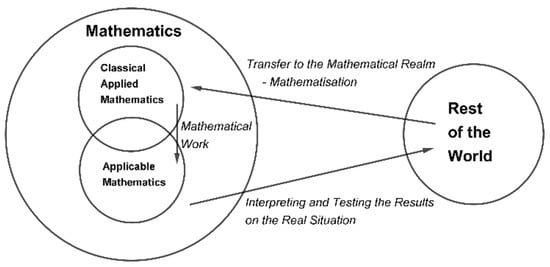
Figure 1.
Pollak’s modeling cycle (source: adopted from [5]).
Pollak’s modeling cycle was an important stimulus that led to a more detailed analysis of the modeling process and initialized the development of other modeling cycles. In the 1990s, Gabriele Kaiser introduced a four-stage mathematical modeling cycle (Figure 2). In comparison with Pollak’s cycle, Kaiser’s cycle includes two stages on the way from the real world to the mathematical realm. At first, the real situation is simplified and idealized in order to form a real-world model, usually represented as a sketch covering the fundamental data, relations, and conditions. After that, based on the real-world model, a mathematical model is formed, which ends the “shift” from reality to mathematics. The other two stages include the problem solution using mathematical methods in order to get mathematical results, which is followed by the interpretation of the results in relation to the initial real situation [6].
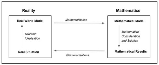
Figure 2.
Kaiser’s modeling cycle (source: adopted from [6]).
Another modeling cycle consisting of six stages was proposed by Blomhøj and Kjeldsen (Figure 3) for the sake of analyzing mathematical modeling competencies. In terms of this cycle, a mental representation of the situation has to be formed first. This stage is followed by systematization, e.g., choice of important objects, relations, etc., with respect to the investigated area and their idealization to allow formation of possible mathematical representations. The next stage—mathematization—refers to the formation of mathematical representations of the examined objects and relations in a thoroughly elaborated manner. The stage of mathematical analysis covers the use of mathematical methods in order to acquire mathematical results and conclusions. Then, the results and conclusions are interpreted with respect to the investigated situation. Finally, the validity of the model has to be verified in contrast with experience, with observed and expected data, or with theoretical knowledge [7,8,9].
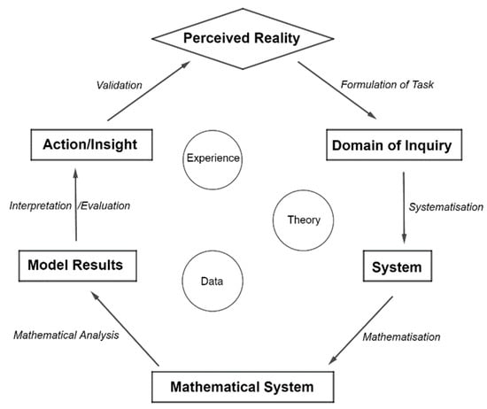
Figure 3.
Blomhøj and Kjeldsen’s modeling cycle (source: adopted from [8]).
One of the latest modeling cycles, based on Kaiser’s model, was introduced by Blum and Leiss (Figure 4). According to this cycle, when shifting from the real-world situation to a mathematical solution, as many as three models have to be formed—a situation model, a real model, and a mathematical model [10].
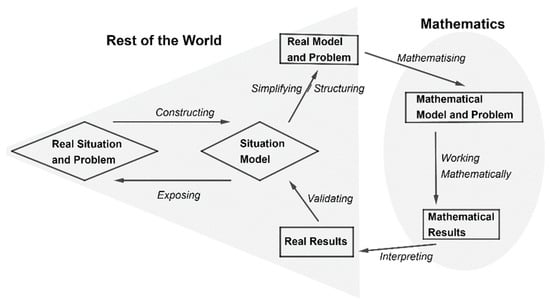
Figure 4.
Blum and Leiss’s modeling cycle (source: adopted from [10]).
In mathematics education, it is vital to encourage individual and original ways of mathematical modeling performed by individual students and thus allow various possible solutions. That is why the teacher is supposed to know the different dimensions of the assigned tasks well and also realize their personal preferences for specific solutions [10]. The teacher must be able to predict mistakes that may be made by students while solving the tasks. It is recommended that, even if the teacher can see a mistake in the students’ solution, they should not tell the students explicitly [11]. Instead, the teacher should ask the students such questions that would make them think more carefully about the procedures they suggest in their solution [12,13]. We believe that if teachers tell their students what they should do and how to get the solution, the students are deprived of the joyful feeling that is usually experienced when a problem is solved. Experiencing the feeling of joy after finding a solution to a problem is beneficial for increasing the students’ interest in problem solving [14].
Through the use of mathematical modeling, we can illustrate to students the importance of mathematics in their everyday lives. By doing this, we can encourage students to learn mathematics and provide direct cognitive support for the students’ ways of thinking. Furthermore, it establishes mathematics in the contemporary culture as a way of understanding real-life situations [1]. Graph theory is often used as a modeling tool not only in school mathematics but also in computer science (e.g., [15,16]). In recent years, the research of mathematics taught within other disciplines has been attracting as much attention as the research of tertiary mathematics education, and it is related to the relevance of mathematics for the science field in particular [17]. The community of computer scientists has discussed the necessity of discrete mathematics courses in computer science undergraduate programs for several decades [18,19,20,21]. Even though Almstrum et al. [22] stated that quite a lot of concepts from discrete mathematics are not covered in mathematics courses and they are embedded in the computing courses, the graph theory has been embedded in nearly all courses in discrete mathematics for computer science in Slovakia [23] and worldwide [19] since the Marion’s seminal paper [24]. Various approaches including inquiry-based learning and team-based learning to discrete mathematics courses have been piloted [19,25,26]. Kuna and Turčáni [27] investigated how implementing interactive multimedia elements into discrete mathematics e-courses can provide an environment enabling students to better understand the given problems considering the fact that visualization can be interpreted as a way of reducing abstraction. Several topics of graph theory were taught using dynamic geometry systems [28], specially designed software [29,30,31], or e-learning courses [32,33,34]. Milková [35] provided software for pairing, subgraphs, isomorphism of graphs, and solving the minimum spanning tree problem and the shortest path problem. Dijsktra’s algorithm for solving the shortest path problem is also implemented in software developed by Dagdilelis and Satratzemi [36].
Despite Niman’s idea [37] (p. 373) that graph theory “could constitute a plausible and exciting alternative in mathematics education” as early as primary level, it permeates school curricula very scarcely [30]. Several authors [38,39] have described their experiences of graph theory algorithms at secondary level; yet, it often happens that students encounter this topic no earlier than in undergraduate discrete mathematics courses. According to Gries and Schneider [25], discrete mathematics courses should motivate students to use rigorous mathematical approaches in solving problems in computer science. Other researchers [40,41] describe empirical experience with unconventionally designed lessons. Lodder [40] uses the historical approach to the introduction of the concept of the tree and the spanning tree. He gives students original problems leading to the discovery of formulas for the number of labeled trees by Cayley and Prufer. However, only a few of these papers include analyzes of students’ thinking [26,42].
Ten possible sources of possible misconceptions in discrete mathematics were recognized by Almstrum et al. [22]; most of them are strongly related to graph theory and graph-theory algorithms. In the area of functions, students perceive problems with properties of functions (injectivity, surjectivity, and bijectivity). These misconceptions can be manifested when the isomorphism of graphs is considered. Another source of misconceptions is the so-called “vacuous truth”, i.e., the fact that all the universally quantified predicates are true for the empty set. Two of the main concepts are related to algorithmic graph theory—inductive reasoning and recursive thinking. Within the concept of inductive reasoning, authors propose that students find it difficult to understand that this method involves increasing the dimension of the problem until the pattern emerges. As for the concept of recursive thinking, students often struggle with the main idea of dynamic programming, which is that the smaller case, i.e., the optimal substructure, has to follow the same structure as the solution of the original problem.
Dagdilelis and Satratzemi [36] identified three characteristics of students’ difficulties with graph theory. The first category comprises difficulties related to the recognition of details of an algorithm. Even if students understand how the algorithm works in a particular case, they have difficulties with describing all the details in general cases. In the second category, there are problems caused by the incomplete understanding of the consecutive stages of the process of computation. The third category of difficulties covers the complications connected with the computational thinking of students, as the usual programming languages are not designed for working with graphs. Hazzan and Hadar [43] stress a dual nature of algorithms. From the procedural perspective, they can be viewed as a sequence of steps that should be executed. From the conceptual viewpoint, an algorithm can be seen as an object with properties to be studied. In recent years, the procedural knowledge has been considered to be equally important as the conceptual understanding [44,45].
One way to diagnose the misconceptions is error analysis (or error pattern analysis), as errors offer a picture of the students’ mind [46]. Error analysis focuses on weaknesses in procedural knowledge [47,48]. It is a process of reviewing students’ item responses in order to identify a pattern of misunderstandings [47]. As suggested by Blum and Boromeo Ferri [10], teachers should know what mistakes students make and predict at which modeling stage students are likely to make the mistakes. An analysis of mistakes can help uncover the causes of mistakes and provide students with valuable feedback [49]. On the other hand, error analysis is not a satisfactory tool to analyze students’ mathematical thinking from the cognitive point of view.
The main aim of this study is to identify types of mistakes that occur in problems related to graph algorithms and to compare the occurrence of the mistakes based on the kind of the problem. In other words, not only the students’ performance is analyzed but also the characteristics of particular problems.
2. Materials and Methods
2.1. Description of the Settings
The study was conducted during a discrete mathematics course for students of applied computer science and future informatics teachers. It is a compulsory course that is usually taken in the first year of the study. Altogether, 135 students were enrolled in the course, 127 of whom took the test. Only the solutions of the latter were subjected to the error analysis.
The discrete mathematics course is spread over two consecutive semesters. In the first semester, topics such as basic logic, sets, relations, and functions, and introduction to number theory are covered. In the spring semester, the basic counting and graph theory are introduced. The graph theory part of the course is oriented towards graph algorithms. In this study, we focus on three problems—the minimum spanning tree problem, the shortest-path problem, and the Chinese postman problem.
The minimum spanning tree problem was introduced to students via its very first application. In the 1920s, the electrification of the northern part of Moravia was being planned. Otakar Borůvka was asked to help. He designed the optimal network and generalized his approach. Students were provided with the unweighted graph. Its vertices represented the towns, and its edges represented the possibility to build a direct electric connection between the towns. The task was to find the minimum amount of edges needed for connecting all the towns. Students found several non-isomorphic solutions. Afterwards, the tree and the spanning tree were defined, and the characterization theorem for trees was proved by the lecturer. Students then solved the same problem on a weighted graph. They were asked to find the cheapest spanning tree. Some of the students managed to come up with Kruskal’s algorithm or some of its variants. The procedure is described in more detail in [42]. After solving the problem, three algorithms were introduced and proved—Kruskal’s algorithm, the reverse-delete algorithm (which is dual to Kruskal’s one), and Jarník-Prim’s algorithm. After the problem-solving activity, the algorithms were formally described and proved by means of mathematical induction.
All three of the algorithms are greedy algorithms, and Jarník-Prim’s one is a typical demonstration of dynamic programming. A more detailed description of all three algorithms can be found, e.g., in the works of Milková [50,51] and Nešetřil et al. [52].
Kruskal’s algorithm starts with all vertices of the graph and no edges. The cheapest edges are added to the graph, while every added edge is required not to create a circle in the constructed subgraph. The reverse-delete algorithm starts with the full graph and deletes the most expensive edges. The deleted edge is required not to be a bridge, i.e., the constructed subgraph has to remain connected.
Jarník-Prim’s algorithm is sometimes referred to as Prim’s algorithm, though it was published by Jarník first. The algorithm uses the idea of dynamic programming. Starting at a single vertex, the cheapest edge connecting the previously constructed subgraph with the unconnected vertices is added. At each step, the constructed subgraph is a minimum spanning tree of the graph induced by vertices used previously, which requires a significant level of recursive thinking. This subgraph is called the optimal substructure in algorithmization.
The second problem covered in the course is the shortest path problem. Similarly to the minimum spanning tree problem, this problem was introduced to students through its application. The lecturer presented how to find the shortest connection between two chosen train stops in a graph representing a part of the Slovak railway network provided by the Slovak railway company. After the solution was created on an unweighted graph, the weighted alternative was solved. Afterwards, the algorithm was formalized and proved by means of mathematical induction.
Dijkstra’s algorithm is another greedy algorithm using dynamic programming. It consists of two stages. Firstly, the distance from one vertex to all other vertices is computed. Secondly, the shortest path is described. In the course, the two possibilities to find the path were introduced. The first one is based on tracing the computation; the second possibility draws on differences between the values of the vertices.
The third problem is the Chinese postman problem. The aim of the algorithm is to find the optimal route for the postman. We used the solution introduced by Edmonds and Johnson [53]. In the first part of the computation, the streets (edges) where the postman is required to walk twice are estimated, and then the Eulerian circle is found. Students worked in groups on designing the algorithms for constructing the Eulerian circle and the Eulerian trail before solving the Chinese postman problem. The Eulerian circle can be found by means of two algorithms. The Euler–Hierholzer’s algorithm is based on Hierholzer’s addition to the Euler’s theorem proof stating the necessary condition for a graph to be Eulerian. The second possibility was Fleury’s algorithm, another greedy algorithm using dynamic programming.
2.2. Data
At the end of the course, as a part of the final assessment, students took a paper-and-pencil test that contained 14 problems: four problems in combinatorics, nine problems in graph theory, and one counting problem where the base sets were graph edges and vertices. In this paper, we analyze three problems that measured the comprehension (the second level of Bloom’s taxonomy) of the abovementioned algorithms. If several algorithms for solving one problem were presented, students could decide on any of them (see Appendix A for the wording of analyzed problems). They could even use their own approaches provided that they were able to prove the correctness of their solution.
The students’ solutions were coded 1 (correct) and 0 (not correct). If a student did not attempt to solve the problem, the code NA (not available) was assigned. Mistakes identified in incorrect solutions were categorized and further analyzed.
2.3. Statistical Analysis
The statistical analysis of the obtained data was performed in the software environment R, packages RVAideMemoire, gplots, and DescTools. The success rates in the three problems were compared by the Cochran Q test, which is the generalization of the McNemar test for two independent samples. The three problems were considered as three independent samples. Subsequently, the post-hoc analysis comparing each pair of problems was performed using the McNemar test. The occurrence and the distribution of students’ mistakes in the three problems were compared by the test of independence. The p-value was estimated by the Monte Carlo method.
Hierarchical cluster analysis is usually employed in order to divide data into meaningful and/or useful groups (clusters). It aims to provide an understanding of the structure and further classification of involved elements (participants, samples, items). The goal is that the objects within a group should be similar (or related) to other objects in the same group, and they should differ from (or be unrelated to) objects in other groups [54]. The analysis was performed in two directions. Firstly, the students were considered as the object to be clustered, and their performances in the three problems were considered as descriptors. Secondly, the problems were considered as objects. In order to evaluate the most appropriate clustering method for each direction of analysis, the correlation coefficients between Euclidean and dendrogram-predicted distances were calculated. The final clustering was visualized by a heatmap and dendrograms.
The level of mathematical knowledge of students was not directly observable; therefore, we investigated a latent variable. Item response theory (IRT) enables us to model the relation between the probability of a particular response to the item and the latent variable. It is often used for assessing the characteristics of a problem [55]. In IRT models, the following three requirements must be met: (i) monotony, e.g., the relation between the probability of the correct answer and the latent variable is monotonously increasing; (ii) unidimensionality, i.e., the test measures only one latent variable; and (iii) local independency, i.e., the items do not correlate on the same levels of latent variable.
There are several IRT models depending on the type of variable, the number of estimated item parameters, and the number of latent variables. If item parameters are estimated, parametric IRT models are used. Parametric IRT models require huge samples [56] and a higher number of items. These requirements were not fulfilled in this case, thus the non-parametric IRT modeling was applied for items and scales. The most frequent approaches are Mokken scaling [57] and kernel smoothing IRT [58]. Mokken scaling is usually used for estimating the number of scales measured by the items. Its biggest drawback is the impossibility to work with data containing missing values. In the reported data, 23% of students had a missing response. On the other hand, kernel smoothing also enabled the analysis of responses with incomplete response patterns.
The non-parametric approach relates the response to an item with the estimate of a latent trait (i.e., characteristic) by means of the kernel density estimator [59]. The estimate of the latent trait is represented by the locally weighted average of latent traits of observations, higher weight being assumed by the observations that occur more closely to the observation whose latent trait value is to be estimated. Kernel smoothing is based on locally weighted averages, which makes it a non-parametric approach, and thus it does not require any IRT model specification. Such a non-parametric approach allows the relation between the latent trait value and the response to an item to be graphically represented as an option characteristic curve (henceforth OCC).
3. Results
In more than one third of the tests, all three solutions were correct. There were only three tests with a mistake in each algorithm (Table 1). The success rates of the problems are summarized in Table 2. The results obtained from Cochran’s Q test (; ) imply that the three problems were not equally demanding. The Chinese postman problem was significantly more problematic in comparison with the remaining two problems. It may be a result of the higher complexity of the algorithm that demands more calculations; therefore, students are more likely to make a mistake.

Table 1.
Frequencies of correctly solved problems in one test (source: own calculation).
Table 2.
Success rates of analyzed problems (source: own calculation).
The two problems (minimum spanning tree problem and shortest path problem) demanding only knowledge and comprehension [60] did not differ significantly (p = 0.121), although the minimum spanning tree (MST) problem was introduced by a problem-solving activity, unlike the shortest path problem. This is in contradiction to the opinion of [61], which claims that problem-based and inquiry-based teachings are not efficient ways to teach mathematics.
3.1. Problem 1: Minimum Spanning Tree Problem
The first problem had the highest success rate amongst the three analyzed problems. The students were allowed to choose from the three algorithms described above—Jarník-Prim’s, Kruskal’s, and reverse-delete algorithm. Surprisingly, the latter was not used at all. We considered it equivalent to Kruskal’s algorithm that was used by 115 students. All six of the solutions using Jarník-Prim’s algorithm were correct. It may be a result of the nature of the algorithm. It requires a higher insight into the idea of dynamic programming and a higher level of recursive thinking compared to Kruskal’s algorithm. Recursive thinking is characterized as an ability to recognize “that the smaller case to which a problem is reduced must have the same … structure as the original problem” [22] (p. 143). When using Kruskal’s algorithm, the following mistakes occurred (Table 3).
Table 3.
Frequencies of mistakes in students’ solutions of the minimum spanning tree problem (source: own calculation).
3.2. Problem 2: Shortest Path Problem
This problem was solved by 112 students; 100 students managed to solve the problem correctly. The solution consists of two stages. Firstly, the vertices of the graph are given weights according to their distance from a chosen vertex. Secondly, the shortest path is determined. In the second stage, students were allowed to choose from two methods. A tracing table was used by 90 students; the method using differences between the weights of vertices was used by 12 students. Two students used their own modifications of the difference methods. The second stage of the algorithm was not performed by three students (Table 4). Students who used the wrong approach to determine the weight of vertices (category a mistake) showed a low level of recursive thinking as defined by Almstrum et al. in [22].
Table 4.
Frequencies of mistakes in students’ solutions of the shortest path problem (source: own calculation).
3.3. Problem 3: Chinese Postman Problem
Out of 127 students who took the test, as many as 117 attempted to solve the problem, and only 76 came up with the correct solution. The mistakes and their frequency are shown in Table 5. The most problematic part of the solution was to identify which edges should be covered twice. Most problems occurred in the determination of the distances between the pairs of odd-degree vertices (there were only three pairs of odd-degree vertices). In some cases, the shortest path was obvious, but there were pairs where the use of Dijkstra’s algorithm was very advantageous. The students could choose how to construct an Eulerian circle in the modified graph with added edges. Out of 95 students who reached this point in their solutions, five students did not solve it at all, 89 used Euler–Hierholzer’s algorithm, and one student used his own modification of this algorithm. Fleury’s algorithm was not used by any student.
Table 5.
Frequencies of mistakes in students’ solutions of the Chinese postman problem (source: own calculation).
3.4. Analysis
The mistakes described in the previous section were assigned to one of the following categories. Category A contains solutions where students started to solve the problem and performed some calculations that were not based on the algorithm presented within the course and did not lead to a correct solution. These kinds of errors are called helplessness and wanderings by [49]. Category B comprises solutions where students knew how to start, but they were not able to solve a part of the solution (e.g., to determine the path after assigning the values to the vertices in the shortest-path problem) or did not solve it correctly, i.e., operational errors. Category C covers mistakes arising from the students’ “instantaneous inattention” that are not based on single numerical or graphical error; they are usually caused by so-called big steps and/or omitting written recording of the calculation process. They are typically made by students in a hurry or by students overestimating their abilities. In order to overcome these types of errors, it is necessary to establish a way to trace the calculations. Category D includes solutions with a single numerical or graphical mistake (e.g., confusion of numbers four and seven).
There are two main sources of these errors: (1) insufficient automatization of lower operations, which demonstrates when the student is focused on solving problems requiring higher processes; (2) underestimating the clarity of their written recordings of the solution. Some authors [47] refer to such mistakes as slips. Categories B (operational errors) and D (slips) seem to be larger than the other two. Mistakes of both of these types can be remedied by more practice, resulting in deeper automatization of mental operations. The category of mistake is not in relation to the problem type (; Monte-Carlo estimation of ). In other words, the relative frequency of each mistake category is similar for each analyzed problem.
3.5. IRT Analysis
Based on data in Table 2, it is obvious that the majority of students came up with the correct solution. For the IRT modeling, we used binary coding. The codes 0 (incorrect), 1 (correct), and NA (did not attempt to solve the problem) were used, leading to maximum final score of 3. The option characteristic curves (OCC) were used for expressing the relation between the response to the item and the expected final score (Figure 5). The final score was considered as a measure of the level of obtained knowledge. Higher scores indicated a higher level of acquired knowledge. In all three of the investigated items, the relation between the expected score and the probability of a correct answer was monotonously increasing.
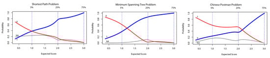
Figure 5.
Option characteristics curves describing the relation between the response to the item and the obtained score in binary coding (source: own visualization).
The monotony of OCCs indicated that the problems were suitable for testing. The better the expected score was, the lower the probability of both incorrect answer and not attempting the solution was. The minimum spanning tree and the shortest path problems seemed again to be similarly demanding. The OCC of the minimum spanning tree problem was the steepest between the fifth percentile and the first quartile. However, the OCC of the Chinese postman problem was the steepest between the first and the third quartile. This implies that the Chinese postman problem discriminated the students according to the latent variable (mathematical ability) on a higher level. Thus, a higher mathematical ability is needed to solve the Chinese postman problem compared to the minimum spanning tree problem or the shortest path problem.
3.6. Hierarchical Cluster Analysis
The identified types of mistakes could be considered as an ordinal variable. Data were coded numerically as 0 (no attempt to solve the problem), 1 (type A mistake), 2 (type B mistake), 3 (type C or D mistake), and 4 (correct solution). The 127 participating students were grouped into five clusters, henceforth denoted as clusters C1 to C5 (Figure 6). Among the five clustering methods (nearest neighbor, weighted pair group method with arithmetic mean, unweighted pair method with arithmetic mean, centroid, and Ward’s grouping), the correlation coefficient between the distance in dendrogram and the Euclidean distance was the highest in the case of the Ward’s grouping for both grouping the students and grouping the problems. Most students (80 out of 127) belonged to cluster C1. The solutions in this cluster were either all correct (50 students), contained only a marginal mistake (type C or D) in the shortest-path problem (two solutions) or the Chinese postman problem (18 solutions), or a B type mistake in the Chinese postman problem (10 solutions). Students in this cluster could be characterized as very successful, mostly making mistakes in solving the Chinese postman problem. The nine students in the second cluster C2 did not start to solve the minimum spanning tree problem or made a B type mistake. There were 13 students grouped in cluster C3. All of them made a mistake or did not attempt to solve the Chinese postman problem. The 19 students in cluster C4 did not solve (eight students) or made a mistake in the shortest path problem. The smallest cluster C5 consisted of only four students, with mistakes in both the Chinese postman problem and the shortest path problem.
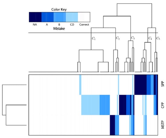
Figure 6.
Heatmap clustering the students’ mistakes in the three problems in graph theory (source: own visualization).
The second direction of the analysis clustered together the minimum spanning tree problem and the Chinese postman problem. According to the IRT analysis, the shortest path problem and the minimum spanning tree are of similar difficulty, thus one might conclude that one of them could be omitted from the test. However, the hierarchical cluster analysis showed that there were different students with mistakes in solving the minimum spanning tree problem and mistakes in solving the shortest path problem.
4. Discussion
This paper builds on the idea that teachers in modeling class should be aware of the different types of mistakes that students can make when solving mathematical problems. Students’ solutions of the three basic problems in algorithmic graph theory were investigated. All the mistakes were made in the mathematical stage of solving the problems. The processes of transition from reality to mathematics (mathematizations) and backwards (interpretations) do not seem to pose any difficulties for the students, unlike in the studies with secondary school students [11]. It could have been a result of the fact that the tasks in the test were set in contexts similar to those in which the motivating tasks had been set, i.e., students knew which algorithms would be the most appropriate.
Eight out of 41 mistakes in solving the Chinese postman problem were caused by a wrong estimation of the distance (the length of the shortest path) between correctly stated pairs of odd-degree vertices. On the other hand, the same students managed to solve the shortest path problem within the same test. This may indicate that the correct application of Dijsktra’s algorithm in context of other problems requires higher cognitive skills [60] compared to simple parroting of the algorithm to a given graph. Even for mathematicians, it can be “frustrating not to be able to find a shorter algorithm” to solve the Chinese postman problem. The Chinese postman problem is an interesting one, because although it is a simple problem, it has an overly complex solution. It is also a good example because it can be solved with different algorithms [62].
The three analyzed tasks make up a good test that excludes the students who have mastered less than the basics. According to the IRT analysis, it is not worth testing students’ abilities in finding the shortest path, since the shortest path problem discriminates as much as the minimum spanning tree problem does, and the shortest path problem is included in a more complex task—the Chinese postman problem. The results of the hierarchical cluster analysis, however, imply a higher similarity between the minimum spanning tree problem and the Chinese postman problem. It is therefore necessary to include all three problems in the test, as they reflect different skills of students in algorithmic graph theory.
The results we acquired suggest that including graph theory in mathematics education is beneficial for the development of students’ modeling skills. In real life, a lot of situations occur that can be modeled by means of graphs, and such a representation can simplify a problem solution. Grasping the principles of graph representations can be a useful problem-solving skill, and it is regrettable that they are scarcely included in secondary education as well as mathematics teacher training.
In this paper, we discussed some insights about students’ work when solving problems with the direct use of graph algorithms. We are aware that a mere look at students’ mistakes is insufficient in defining the sources of students’ difficulties related to higher cognitive skills and should be accomplished by means of a diagnostic interview. A deeper analysis of students’ recursive reasoning and inductive thinking employed in solving more demanding problems in discrete mathematics is a subject for further research.
Author Contributions
The authors contributed in following manners: conceptualization, J.M. and K.P.; methodology, J.M.; software, J.M. and Ľ.R.; validation, Ľ.R. and Z.N.; formal analysis, Ľ.R. and J.M.; investigation, J.M.; resources, J.M.; data curation, Ľ.R.; writing—original draft preparation, J.M. and K.P.; writing—review and editing, Z.N.; visualization, Ľ.R. and J.M.; supervision, J.M.; project administration, J.M.; funding acquisition, J.M.
Funding
This work was supported by the Slovak Research and Development Agency under the contract No. APVV-15-0368.
Acknowledgments
The preliminary analysis of the data was presented at the 14th International Conference Efficiency and Responsibility in Education, held in Prague, Czech Republic, on 8–9 June 2017, though the theoretical background has been refined and analysis was extended.
Conflicts of Interest
The authors declare no conflict of interest.
Appendix A
The texts of the problems given to students are added here.
Problem 1 (Minimum spanning tree problem)
The following picture (Figure A1) shows a computer network scheme. Data are sent from the source A to all the devices in the network. Design a path for the data that minimizes the network load. The numbers in the graph represent the particular response times [63].
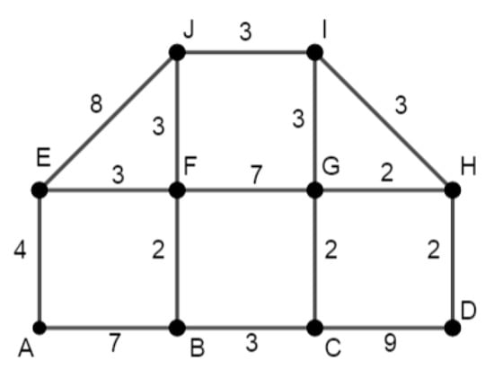
Figure A1.
Scheme to problem 1.
Problem 2 (Shortest path problem)
Given a weighted graph (Figure A2) that represents a railway network, find the shortest path between the stops A and F. The weights of the edges represent the distances between the railway stops.
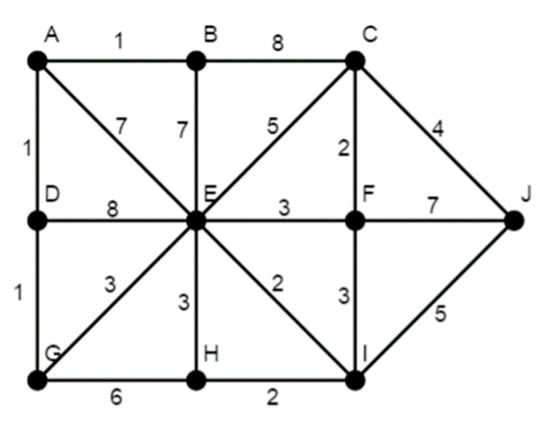
Figure A2.
Scheme to problem 2.
Problem 3 (Chinese postman problem)
A postman has to deliver mail to people living in his beat, which is represented in the graph (Figure A3). The streets are shown as edges whose weights represent the time needed to walk along the particular street. The vertices of the graph represent crossroads, i.e., spots where the streets meet or intersect each other. The postman sets out from the post office (P). Plan his route so that the delivery takes as little time as possible.
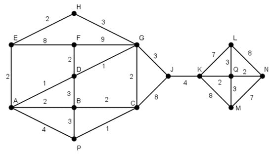
Figure A3.
Scheme to problem 3.
References
- Blomhøj, M. Different perspectives in research on the teaching and learning mathematical modeling. In Mathematical Applications and Modeling in the Teaching and Learning of Mathematics; Proceedings from Topis Study Group 21 at the 11th ICME, Monterrey, Mexiko, 6–13 July, 2008; Blomhøj, M., Carreira, S., Eds.; Roskilde University: Roskilde, Denmark, 2009; pp. 6–13. [Google Scholar]
- Lesh, R.; Carmona, G.; Post, T. Models and Modeling. In Proceedings of the Annual Meeting of the North American Chapter of the International Group for PME, Athens, Greece, 26–29 October 2002; pp. 89–98. [Google Scholar]
- Fischer, R.; Malle, G. Mensch und Mathematik; Bibliographisches Institut: Mannheim, Germany, 1985; ISBN 3-411-03117-4. [Google Scholar]
- Binns, B.; Burkhardt, H.; Gillespie, J.; Swan, M.B. Mathematical modeling in the School Classroom: Developing Effective Support for Representative Teachers. In Applications and Modeling in Learning and Teaching mathematics; Proceedings of the 3rd ICTMA, Kassel University, Germany, 8–11 September, 1987; Blum, W., Niss, M., Huntley, I., Eds.; Halsted Press: Chichester, UK, 1989; pp. 136–143. [Google Scholar]
- Voskoglou, M.G. Mathematical Modeling as a Teaching Method of Mathematics. J. Res. Innov. Teach. 2015, 8, 35–50. [Google Scholar]
- Kaiser, G. Mathematical Modeling in School—Examples and Experiences. In Mathematikunterricht im Spannungsfeld von Evolution und Evaluation. Festschrift für Werner Blum; Henn, H.-W., Ed.; Franzbecker: Hildesheim, Germany, 2005; pp. 99–108. [Google Scholar]
- Blomhøj, M.; Jensen, T.H. Developing mathematical modeling competence: Conceptual clarification and educational planning. Teach. Math. Appl. 2003, 22, 123–139. [Google Scholar] [CrossRef]
- Blomhøj, M.; Kjeldsen, T.H. Teaching mathematical modeling through project work. ZDM 2006, 38, 163–177. [Google Scholar] [CrossRef]
- Blomhøj, M.; Kjeldsen, T.H. Learning the Integral Concept through Mathematical Modeling. In Proceedings of the 5th CERME, Larnaca, Cyprus, 22–26 February 2007; Pitta-Pantazi, D., Philippou, G., Eds.; pp. 2070–2079. [Google Scholar]
- Blum, W.; Borromeo Ferri, R. Mathematical Modeling: Can it Be Taught and Learnt? J. Math. Model. Appl. 2009, 1, 45–58. [Google Scholar]
- Plothová, L. Development of Abilities to Model and to Algebrize Relations and Dependencies as Part of Standard Competences in Education of Mathematics on Grammar-School. Ph.D. Thesis, Constantine the Philosopher University, Nitra, Slovakia, 2017. [Google Scholar]
- Boaler, J. Mathematical Mindsets, 1st ed.; Jossey-bass, A Wiley Brand: San Francisco, CA, USA, 2016; ISBN 978-0-470-89452-1. [Google Scholar]
- Samkova, L. The current state of IBME in the Czech Republic. In Implementing Inquiry in Mathematics Education; Baptist, P., Raab, D., Eds.; University of Bayreuth: Bayreuth, Germany, 2012; pp. 82–93. [Google Scholar]
- Bruder, R.; Prescott, A. Research evidence on the benefits of IBL. ZDM 2013, 45, 811–822. [Google Scholar] [CrossRef]
- Balogh, Z.; Turčáni, M.; Magdin, M. Design and Creation of a Universal Model of Educational Process with the Support of Petri Nets. Lect. Notes Electr. Eng. 2014, 269, 1049–1060. [Google Scholar] [CrossRef]
- Li, X.; Li, G.; Zhang, S. Routing Space Internet Based on Dijkstra’s Algorithm. In Proceedings of the 2009 First Asian Himalayas International Conference on Internet, Kathmandu, Nepal, 3–5 November 2009; pp. 1–4. [Google Scholar]
- Biza, I.; Giraldo, V.; Hochmuth, R.; Khakbaz, A.; Rasmussen, C. Research on Teaching and Learning Mathematics at the Tertiary Level: State-of-the-Art and Looking Ahead; ICME-13 Topical, Surveys; Kaiser, G., Ed.; Springer Open: Berlin, Germany, 2016; pp. 1–32. [Google Scholar] [CrossRef]
- Marion, W.A. Discrete mathematics for computer science majors—Where are we? How do we proceed? In Proceedings of the SIGCSE ‘89 Twentieth SIGCSE Technical Symposium on Computer Science Education, Louisville, KY, USA, 23–24 February 1989; Volume 21, pp. 273–277. [Google Scholar]
- Li, C.-C.; Mehrotra, K.; Jong, C. Discrete mathematics as a transitional course. Ideas 2012, 3, 40. [Google Scholar]
- Ivanov, O.A.; Ivanova, V.V.; Saltan, A.A. Discrete mathematics course supported by CAS MATHEMATICA. Int. J. Math. Educ. Sci. Technol. 2017, 48, 953–963. [Google Scholar] [CrossRef]
- Ho, W.K.; Toh, P.C.; Teo, K.M.; Zhao, D.; Hang, K.H. Beyond School Mathematics. In Mathematics Education in Singapore; Toh, T.L., Kaur, B., Tay, E.G., Eds.; Springer: Singapore, 2019; pp. 67–100. ISBN 978-981-13-3573-0. [Google Scholar]
- Almstrum, V.L.; Henderson, P.B.; Harvey, V.; Heeren, C.; Marion, W.; Riedesel, C.; Soh, L.-K.; Tew, A.E. Concept inventories in computer science for the topic discrete mathematics. ACM SIGCSE Bull. 2006, 38, 132–145. [Google Scholar] [CrossRef]
- Turčáni, M.; Kuna, P. Analysis of subject discrete mathematics parts and proposal of e-course model following Petri nets for informatics education. ERIES J. 2013, 6, 1–13. [Google Scholar] [CrossRef]
- Marion, W. Discrete mathematics a mathematics course or a computer science course? Probl. Resour. Issues Math. Undergr. Stud. 1991, 1, 314–324. [Google Scholar] [CrossRef]
- Gries, D.; Schneider, F.B. A new approach to teaching discrete mathematics. Probl. Resour. Issues Math. Undergr. Stud. 1995, 5, 113–138. [Google Scholar] [CrossRef]
- Paterson, J.; Sneddon, J. Conversations about curriculum change: Mathematical thinking and team-based learning in a discrete mathematics course. Int. J. Math. Educ. Sci. Technol. 2011, 42, 879–889. [Google Scholar] [CrossRef]
- Kuna, P.; Turčáni, M. Design of new methods of teaching the subject Discrete Math. In Proceedings of the 11th ICETA, Stara Lesna, Slovakia, 24–25 October 2013; pp. 247–251. [Google Scholar]
- Falcón, R.; Ríos, R. The use of GeoGebra in Discrete Mathematics. GeoGebra Int. J. Rom. 2015, 4, 39–50. [Google Scholar]
- Baudon, O.; Laborde, J.M. Cabri-graph, a sketchpad for graph theory. Math. Comp. Simul. 1996, 42, 765–774. [Google Scholar] [CrossRef]
- Fest, A.; Kortenkamp, U. Teaching graph algorithms with Visage. Teach. Math. Comp. Sci. 2009, 7, 35–50. [Google Scholar] [CrossRef]
- Quinn, A. Using Apps to Visualize Graph Theory. Math. Teach. 2015, 108, 626–631. [Google Scholar] [CrossRef]
- Vidermanová, K.; Melušová, J.; Vasková, V. Employing learning management system Moodle in discrete mathematics course in undergraduate education from students’ point of view. In Proceedings of the APLIMAT, Bratislava, Slovakia, 6–9 February 2007; pp. 413–417, ISBN 978-80-969562-8-9. [Google Scholar]
- Karagiannis, P.; Markelis, I.; Paparrizos, K.; Samaras, N.; Sifaleras, A. E-learning technologies: Employing matlab web server to facilitate the education of mathematical programming. Int. J. Math. Educ. Sci. Technol. 2006, 37, 765–782. [Google Scholar] [CrossRef]
- Hanzel, P.; Voštinár, P. Elektronický kurz “Vybrané kapitoly z diskrétnej matematiky” [Electronic Course in Discrete Mathematics]. Stud. Sci. Fac. Peadagogicae 2016, 11, 88–96. [Google Scholar]
- Milková, E. Constructing knowledge in graph theory and combinatorial optimization. WSEAS Trans. Math. 2009, 8, 424–434. [Google Scholar]
- Dagdilelis, V.; Satratzemi, M. DIDAGRAPH: Software for teaching graph theory algorithms. ACM SIGCSE Bull. 1998, 30, 64–68. [Google Scholar] [CrossRef]
- Niman, J. Graph theory in the elementary school. Educ. Stud. Math. 1975, 6, 351–373. [Google Scholar] [CrossRef]
- Yanagimoto, T.; Nakamoto, A.; Mazura, N. A study on teaching graph theory—For primary & junior high school students. In Proceedings of the TSG 13 in ICME-10, Copenhagen, Denmark, 4–11 July 2004; Niss, M., Ed.; Roskilde University: Roskilde, Denmark, 2008; pp. 346–350, ISBN 978-87-7349-733-3. [Google Scholar]
- Geschke, A.; Kortenkamp, U.; Lutz-Westphal, B.; Materlik, D. Visage—Visualization of algorithms in discrete mathematics. ZDM 2005, 37, 395–401. [Google Scholar] [CrossRef]
- Lodder, J. Networks and spanning trees: The juxtaposition of Prüfer and Borůvka. Probl. Resour. Issues Math. Undergr. Stud. 2014, 24, 737–752. [Google Scholar] [CrossRef]
- Cigas, J.; Hsin, W.-J. Teaching proofs and algorithms in discrete mathematics with online visual logic puzzles. J. Educ. Resour. Comput. 2005, 5, 1–12. [Google Scholar] [CrossRef]
- Vidermanová, K.; Melušová, J. Teaching graph theory with Cinderella and Visage: An undergraduate case. In New Trends in Mathematics Education: DGS in Education; Vallo, D., Šedivý, O., Vidermanová, K., Eds.; Univerzita Konštantína Filozofa v Nitre: Nitra, Slovakia, 2011; pp. 79–85. ISBN 978-80-8094-853-5. [Google Scholar]
- Hazzan, O.; Hadar, I. Reducing Abstraction when Learning Graph Theory. J. Comp. Math. Sci. Teach. 2005, 24, 255–272. [Google Scholar]
- Star, J.R. Foregrounding Procedural Knowledge. J. Res. Math. Educ. 2007, 38, 132–135. [Google Scholar] [CrossRef]
- Rittle-Johnson, B.; Schneider, M.; Star, J. Not a One-Way Street: Bidirectional Relations between Procedural and Conceptual Knowledge of Mathematics. Educ. Psychol. Rev. 2015, 27, 587–597. [Google Scholar] [CrossRef]
- Brodie, K. Learning about learner errors in professional learning communities. Educ. Stud. Math. 2014, 85, 221–239. [Google Scholar] [CrossRef]
- Ketterlin-Geller, L.R.; Yovanoff, P. Diagnostic assessments in mathematics to support instructional decision making. Pract. Assess. Res. Eval. 2009, 14, 1–11. [Google Scholar]
- Borasi, R. Exploring mathematics through the analysis of errors. Learn. Math. 1987, 7, 2–8. [Google Scholar]
- Hejný, M. Teória Vyučovania Matematiky 2 [Theory of Mathematics Education 2]; SPN: Bratislava, Slovakia, 1989; ISBN 80-08-01344-3. [Google Scholar]
- Milková, E. The minimum spanning tree problem: Jarník’s solution in historical and present context. Electron. Notes Discret. Math. 2007, 28, 309–316. [Google Scholar] [CrossRef]
- Milková, E. Combinatorial Optimization: Mutual Relations among Graph Algorithms. WSEAS Trans. Math. 2008, 7, 293–302. [Google Scholar]
- Nešetřil, J.; Milková, E.; Nešetřilová, H. Otakar Borůvka on minimum spanning tree problem: Translation of both the 1926 papers, comments, history. Discret. Math. 2001, 233, 3–36. [Google Scholar] [CrossRef]
- Edmonds, J.; Johnson, E.L. Matching, Euler tours and the Chinese postman. Math. Program. 1973, 5, 88–124. [Google Scholar] [CrossRef]
- Kráľ, P.; Kanderová, M.; Kaščáková, A.; Nedelová, G.; Valenčáková, V. Viacrozmerné Štatistické Metódy so Zameraním na Riešenie Problémov Ekonomickej Praxe [Multivariate Statistical Methods with Focus on Solving Problems of Economic Practice]; Univerzita Mateja Bela v Banskej Bystrici: Banská Bystrica, Slovakia, 2009; ISBN 978-80-8083-840-9. [Google Scholar]
- Novotná, J.; Chvál, M. Impact of order of data in word problems on division of a whole into unequal parts. ERIES J. 2018, 11, 85–92. [Google Scholar] [CrossRef]
- Meijer, R.R.; Baneke, J.J. Analyzing psychopathology items: A case for nonparametric item response theory modeling. Psychol. Methods 2004, 9, 354–368. [Google Scholar] [CrossRef] [PubMed]
- Mokken, R.J. A Theory and Procedure of Scale Analysis; De Gruyter Mouton: Berlin, Germany, 1971; ISBN 978-3-11-081320-3. [Google Scholar]
- Ramsay, J.O. A functional approach to modeling test data. In Handbook of Modern Item Response Theory; van der Linden, W.J., Hambleton, R.K., Eds.; Springer: New York, NY, USA, 1997; pp. 381–394. ISBN 978-1-4757-2691-6. [Google Scholar]
- Simonoff, J.S. Smoothing Methods in Statistics; Springer: New York, NY, USA, 1996; ISBN 978-1-4612-4026-6. [Google Scholar]
- Bloom, B.S.; Engelhart, M.D.; Furst, E.J.; Hill, W.H.; Krathwohl, D.R. Taxonomy of Educational Objectives. Handbook I: Cognitive Domain; McKay: New York, NY, USA, 1956; pp. 20–24. [Google Scholar]
- Kirschner, P.A.; Sweller, J.; Clark, R.E. Why minimal guidance during instruction does not work: An analysis of the failure of constructivist, discovery, problem-based, experiential, and inquiry-based teaching. Educ. Psychol. 2006, 41, 75–86. [Google Scholar] [CrossRef]
- Thimbleby, H. The directed Chinese postman problem. Softw. Pract. Exp. 2003, 33, 1081–1096. [Google Scholar] [CrossRef]
- Rosen, K.H. Discrete Mathematics and Its Applications, 7th ed.; McGraw Hill Companies: New York, NY, USA, 2007; ISBN 978-0-07-338309-5. [Google Scholar]
© 2019 by the authors. Licensee MDPI, Basel, Switzerland. This article is an open access article distributed under the terms and conditions of the Creative Commons Attribution (CC BY) license (http://creativecommons.org/licenses/by/4.0/).