A Novel Monarch Butterfly Optimization with Global Position Updating Operator for Large-Scale 0-1 Knapsack Problems

Abstract

As a significant subset of the family of discrete optimization problems, the 0-1 knapsack problem (0-1 KP) has received considerable attention among the relevant researchers. The monarch butterfly optimization (MBO) is a recent metaheuristic algorithm inspired by the migration behavior of monarch butterflies. The original MBO is proposed to solve continuous optimization problems. This paper presents a novel monarch butterfly optimization with a global position updating operator (GMBO), which can address 0-1 KP known as an NP-complete problem. The global position updating operator is incorporated to help all the monarch butterflies rapidly move towards the global best position. Moreover, a dichotomy encoding scheme is adopted to represent monarch butterflies for solving 0-1 KP. In addition, a specific two-stage repair operator is used to repair the infeasible solutions and further optimize the feasible solutions. Finally, Orthogonal Design (OD) is employed in order to find the most suitable parameters. Two sets of low-dimensional 0-1 KP instances and three kinds of 15 high-dimensional 0-1 KP instances are used to verify the ability of the proposed GMBO. An extensive comparative study of GMBO with five classical and two state-of-the-art algorithms is carried out. The experimental results clearly indicate that GMBO can achieve better solutions on almost all the 0-1 KP instances and significantly outperforms the rest.

1. Introduction

The 0-1 knapsack problem (0-1 KP) is a classical combinatorial optimization task and a challenging NP-complete problem as well. That is to say, it can be solved by nondeterministic algorithms in polynomial time. Similar to other NP-complete problems, such as vertex cover (VC), hamiltonian circuit (HC), and set cover (SC), the 0-1 KP is intractable. In other words, no polynomial-time exact algorithms have been found for it thus far. This problem was originated from the resource allocation involving financial constraints and since then, has been extensively studied in an array of scientific fields, such as combinatorial theory, computational complexity theory, applied mathematics, and computer science [1]. Additionally, it has been found to have many practical applications, such as project selection [2], investment decision-making [3], and network interdiction problem [4]. Mathematically, we can describe the 0-1 KP as follows:

$$\begin{array}{l}Maximizef(x)={\displaystyle \sum _{i=1}^n}{p}_i{x}_i\\ subjectto{\displaystyle \sum _{i=1}^n}{w}_i{x}_i\le C,\\ x_i=0or1,i=1,\dots ,n,\end{array}$$

(1)

where n is the number of items, p_i, and w_i denote the profit and weight of item i, respectively. C represents the total capacity of the knapsack. The 0-1 variable x_i indicates whether the item i is put into the knapsack, i.e., if any item i is selected and belongs to the knapsack, x_i = 1, otherwise, x_i = 0. The objective of the 0-1 KP is to maximize the total profits of the items placed in the knapsack, subject to the condition that the sum of the weights of the corresponding items does not exceed a given capacity C.

Since the 0-1 KP was reported by Dantzig [5] in 1957, a large number of researchers have focused on addressing it in diverse areas. Some of the main early methods in this field are exact methods, such as the branch and bound method (B&B) [6] and the dynamic programming (DP) method [7]. It is a breakthrough to introduce the concept of the core by Martello et al. [8]. In addition, some effective algorithms have been proposed for 0-1 KP [9], the multidimensional knapsack problem (MKP) [10]. With the rapid development of computational intelligence, some modern metaheuristic algorithms have been proposed for addressing the 0-1 KP. Some of those related algorithms include genetic algorithm (GA) [11], differential evolution (DE) [12], shuffled frog-leaping algorithm (SFLA) [13], cuckoo search (CS) [14,15], artificial bee colony (ABC) [16,17], harmony search (HS) [17,18,19,20,21], and bat algorithm (BA) [22,23]. Many research methods are applied to the 0-1 KP problem. Zhang et al. converted the 0-1 KP problem into a directed graph by the network converting algorithm [24]. Kong et al. proposed an ingenious binary operator to solve the 0-1 KP problem by simplified binary harmony search [20]. Zhou et al. presented a complex-valued encoding scheme for the 0-1 KP problem [22].

In recent years, inspired by natural phenomena, a variety of novel meta-heuristic algorithms have been reported, e.g., bat algorithm (BA) [23], amoeboid organism algorithm [24], animal migration optimization (AMO) [25], artificial plant optimization algorithm (APOA) [26], biogeography-based optimization (BBO) [27,28], human learning optimization (HLO) [29], krill herd (KH) [30,31,32], monarch butterfly optimization (MBO) [33], elephant herding optimization (EHO) [34], invasive weed optimization (IWO) algorithm [35], earthworm optimization algorithm (EWA) [36], squirrel search algorithm (SSA) [37], butterfly optimization algorithm (BOA) [38], salp swarm algorithm (SSA) [39], whale optimization algorithm (WOA) [40], and others. A review of swarm intelligence algorithms can be referred to [41].

As a novel biologically inspired computing approach, MBO is inspired by the migration behavior of the monarch butterflies with the change of the seasons. The related investigations [42,43] have demonstrated that the advantage of MBO lies in its simplicity, being easy to carry out, and efficiency. In order to address the 0-1 KP, which falls within the domain of the discrete combinatorial optimization problems with constraints, this paper presents a specially designed monarch butterfly optimization with global position updating operator (GMBO). What needs special mention is that GMBO is a supplement and perfection to previous related work, namely, a binary monarch butterfly optimization (BMBO) and a novel chaotic MBO with Gaussian mutation (CMBO) [42]. The main difference and contributions of this paper are as follows, compared with BMBO and CMBO.

Firstly, the original MBO was proposed to address the continuous optimization problems, i.e., it cannot be directly applied in the discrete space. For this reason, in this paper, a dichotomy encoding strategy [44] was employed. More specifically, each monarch butterfly individual is represented as two-tuples consisting of a real-valued vector and a binary vector. Secondly, although BMBO demonstrated excellent performance in solving 0-1 KP, it did not show a prominent advantage [42]. In other words, some techniques can be combined with BMBO for the purpose of improving its global optimization ability. Based on this, an efficient global position updating operator [16] was introduced to enhance the optimization ability and ensure its rapid convergence. Thirdly, a novel two-stage repair operator [45,46] called the greedy modification operator (GMO), and greedy optimization operator (GOO), respectively, was adopted. The former repairs the infeasible solutions while the latter optimizes the feasible solutions during the search process. Fourthly, empirical studies reveal that evolutionary algorithms have certain dependencies on the selection of parameters. Moreover, certain coupling between the parameters still exists. However, suitable parameter combination for a particular problem was not analyzed in BMBO and CMBO. In order to verify the influence degree of four important parameters on the performance of GMBO, an orthogonal design (OD) [47] was applied, and then the appropriate parameter settings were examined and recommended. Fifthly, generally speaking, the approximate solution of an NP-hard problem can be obtained by evolutionary algorithms. However, the most important thing is to obtain higher quality approximate solutions, which are closer to the optimal solutions more profitably. In BMBO, the optimal solutions of all the 0-1 KP instances were not provided. It is difficult to judge the quality of an approximate solution obtained by an evolutionary algorithm. In GMBO, the optimal solutions of 0-1 KP instances are calculated by a dynamic programming algorithm. Meanwhile, the approximation ratio based on the best values and the worst values are provided, which clearly reflect the degree of the closeness of the approximate solutions to the optimal solutions. In addition, the application of statistical methods in GMBO is one of the differences between GMBO and BMBO, CMBO, including Wilcoxon’s rank-sum tests [48] with a 5% significance level. Moreover, boxplots can visualize the experimental results from the statistical perspective.

The rest of the paper is organized as follows. Section 2 presents a snapshot of the original MBO, while Section 3 introduces the GMBO for large-scale 0-1 KP in detail. Section 4 reports the outcomes of a series of simulation experiments as well as to compare results. Finally, the paper ends with Section 5 after providing some conclusions, along with some directions for further work.

2. Monarch Butterfly Optimization

Animal migration involves mainly long-distance movement, usually in groups, on a regular seasonal basis. MBO [33,43] is a population-based intelligent stochastic optimization algorithm that mimics the seasonal migration behavior of monarch butterflies in nature. It should be noted that the entire population is divided into two subpopulations, named subpopulation_1 and subpopulation_2, respectively. Based on this, the optimization process consists of two operators, which operate on subpopulation_1 and subpopulation_2, respectively. The information is interchanged among the individuals of subpopulation_1 and subpopulation_2 by applying the migration operator. The butterfly adjusting operator delivers the information of the best individual to the next generation. Additionally, Lévy flights [49,50] are introduced into MBO. The main steps of MBO are outlined as follows:

Step 1.

Initialize the parameters of MBO. There are five basic parameters to be considered while addressing various optimization problems, including the number of the population (NP), the ratio of the number of monarch butterflies in subpopulation_1 (p), migration period (peri), the monarch butterfly adjusting rate (BAR), the max walk step of the Lévy flights (Smax).

Step 2.

Initialize the population with NP randomly generated individuals according to a uniform distribution in the search space.

Step 3.

Sort the individuals according to their fitness in descending order (Here assumptions for the maximum). The better NP₁ (p*NP) individuals constitute subpopulation_1, and NP₂ (NP-NP₁) individuals make up subpopulation_2.

Step 4.

The position updating of individuals in subpopulation_1 is determined by the migration operator. The specific procedure is described in Algorithm 1.

Algorithm 1. Migration Operator

Begin

for i = 1 to NP1 (for all monarch butterflies in subpopulation_1)

for j = 1 to d (all the elements in ith monarch butterfly)

r = rand * peri, where rand ~ U(0,1)

if r ≤ p then

$x_{i,j}=x_{r1,j}$, where r1~U[1, 2,…, NP1]

else

$x_{i,j}=x_{r2,j}$, where r2~U[1, 2,…, NP2]

end if

end for j

end for i

End.

Step 5.

The moving direction of the individuals in subpopulation_2 depends on the butterfly adjusting operator. The detailed procedure is shown in Algorithm 2.

Step 6.

Recombine two subpopulations into one population

Step 7.

If the termination criterion is already satisfied, output the best solution found, otherwise, go to Step 3.

where dx is calculated by implementing the Lévy flights. It should be noted that the Lévy flights, which originated from the Lévy distribution, are an impactful random walk model, especially on undiscovered, higher-dimensional search space. The step size of Lévy flights refers to Equation (2).

$$StepSize=ceil(exprnd(2\ast Maxgen))$$

(2)

where function exprnd(x) returns random numbers of an exponential distribution with mean x and ceil(x) gets a value to the nearest integer greater than or equal to x. Maxgen is the maximum number of iterations.

The parameter ω is the weighting factor which has inverse proportional relationship to the current generation.

Algorithm 2. Butterfly Adjusting Operator

Begin

for i = 1 to NP2 (for all monarch butterflies in subpopulation_2)

for j = 1 to d (all the elements in ith monarch butterfly)

if rand ≤ p then where rand ~ U(0,1)

$x_{i,j}=x_{best,j}$

else

$x_{i,j}=x_{r3,j}$ where r3 ~ U[1,2,…, NP2]

if rand > BAR then

$x_{i,j}=x_{i,j}+\omega \times (d{x}_j-0.5)$

end if

end if

end for j

end for i

End.

3. A Novel Monarch Butterfly Optimization with Global Position Updating Operator for the 0-1 KP

In this section, we give the detailed design procedure of the GMBO for the 0-1 KP. Firstly, a dichotomy encoding scheme [46] is used to represent each individual. Secondly, a global position updating operator [16] is embedded in GMBO in order to increase the probability of finding the optimal solution. Thirdly, the two-stage individual optimization method is employed, which successively tackles the infeasible solutions and then further improves the existing feasible solutions. Finally, the basic framework of GMBO for 0-1 KP is formed.

3.1. Dichotomy Encoding Scheme

KP belongs to the category of discrete optimization. The solution space is a collection of discrete points rather than a contiguous area. For this reason, we should either redefine the evolutionary operation of MBO or directly apply a continuous algorithm to discrete problems. In this paper, we prefer the latter for its simplicity of operation, comprehensibility, and generality.

As previously mentioned, each monarch butterfly individual is expressed as a two-tuple <X, Y>. Here, real number vectors X still constitute the search space as in the original MBO, which can be regarded as a phenotype similar to the genetic algorithm. Binary vectors, Y, form the solution space, which can be seen as a genotype common in the evolutionary algorithm. It should be noted that Y may be a valid solution because 0-1KP is a constraint optimization problem. Here we abbreviate the monarch butterfly population to MBOP. Then the structure of MBOP is given as follows:

$$MBOP=\left[\begin{array}{l}(x_{1,1},y_{1,1})(x_{1,2},y_{1,2})\cdots (x_{1,d},y_{1,d})\\ (x_{2,1},y_{2,1})(x_{2,2},y_{2,2})\cdots (x_{2,d},y_{2,d})\\ \cdots \cdots \cdots \cdots \\ (x_{NP,1},y_{NP,1})(x_{NP,2},y_{NP,2})\cdots (x_{NP,d},y_{NP,d})\end{array}\right]$$

(3)

The first step to adopting a dichotomous encoding scheme is to transfer the phenotype to genotype. Therefore, a surjective function g is used to realize the mapping relationship from each element of X to the corresponding element of Y.

$$g(x)=\{\begin{array}{l}1ifsig(x)\ge 0.5\\ 0else\end{array}$$

(4)

where $sig(x)=1/(1+e^{-x})$ is the sigmoid function. The sigmoid function is often used as the threshold function of neural networks. It was applied to the binary particle swarm optimization (BPSO) [51] to convert the position of a particle from a real-valued vector to a 0-1 vector. It should be noted that there are other conversion functions [52] can be used.

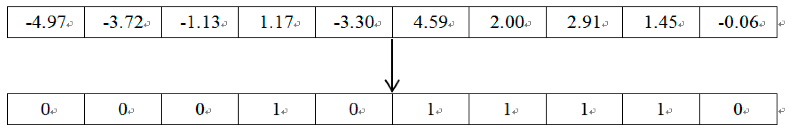
Now assume a 0-1 KP problem with 10 items, Figure 1 shows the above process, in which each $x_i\in \left[-5.0,5.0\right]$ ($1\le i\le 10$) is randomly chosen based on the uniform distribution.

3.2. Global Position Updating Operator

The main feature of particle swarm optimization (PSO) is that the particle always tends to converge to two extreme positions viz. the best position ever found by itself and the global best position. Inspired by the behavior of swarm intelligence of PSO, a novel position updating operator was recently proposed and successfully embedded in HS for solving 0-1 KP [16]. After that, the position updating operator combines with CS [14] to deal with 0-1 KP.

It is well-known that the evolutionary algorithm can yield strong optimization performance under the condition of the balance between exploitation and exploration, or attraction and diffusion [53]. The original MBO concentrates much on the exploration ability but weak exploitation capability [33,43]. With the aim of enhancing the exploitation capability of MBO, we introduce a global position updating operator mentioned above. The procedure is shown in Algorithm 3, where “best” and “worst” represent the global best individual and the global worst individual, respectively. r₄, r_5, and rand are uniform random real numbers in [0, 1]. The p_m parameter is mutation probability.

Algorithm 3. Global Position Updating Operator

Begin

for i = 1 to NP (for all monarch butterflies in the whole population)

for j = 1 to d (all the elements in ith monarch butterfly)

$ste{p}_j=\left|x_{best,j}-x_{worst,j}\right|$

if (rand ≥ 0.5)        where rand ~ U(0,1)

$x_j=x_{best,j}+r_4\times ste{p}_j$ where r4 ~ U(0,1)

else

$x_j=x_{best,j}-r_4\times ste{p}_j$

end if

if ($rand\le p_m$)

$x_j=L_j+r_5\times (U_j-L_j)$ where r5 ~ U(0,1)

end if

end for j

end for i

End.

3.3. Two-Stage Individual Optimization Method Based on Greedy Strategy

Since KP is a constrained optimization problem, it may lead to the occurrence of infeasible solutions. There are usually two major methods: Redefining the objective function by penalty function method (PFM) [54,55] and individual optimization method based on the greedy strategy (IOM) [56,57]. Unfortunately, the former shows poor performance when encountering large-scale KP problems. In this paper, we adopt IOM to address infeasible solutions.

A simple greedy strategy, namely GS [58], is proposed to choose the item with the greatest density p_i/w_i first. Although the feasibility of all individuals can be guaranteed, it is obvious that there are several imperfections. Firstly, for a feasible individual, there is a possibility that the corresponding objective function value may turn to be worse by applying GS. Secondly, the lack of further optimization for all individuals can lead to unsatisfactory solutions.

In order to overcome the shortcomings of GS, the two-stage individual optimization method is proposed by He et al. [45,46]. A greedy modification operator (GMO) is used to repair the infeasible individuals in the first stage. It is followed by the application of the greedy optimization operator (GOO), which further optimizes the feasible individuals. The method proceeds as follows.

Step 1.

Quicksort algorithm is used to sort all items in the non-ascending order according to p_i/w_i, and the index of items is stored in an array H[1], H[2]…, H[n], respectively.

Step 2.

For an infeasible individual $\mathbf{X}=\{x_1,x_2,\dots ,x_n\}\in {\{0,1\}}^n$, GMO is applied.

Step 3.

For a feasible individual $\mathbf{X}=\{x_1,x_2,\dots ,x_n\}\in {\{0,1\}}^n$, GOO is performed.

After the above repair process, it is easy to verify that each optimized individual is feasible. The significance of GMO and GOO seems particularly prominent while solving high dimensional KP problems [45,46]. The pseudo-code of GMO and GOO can be shown in Algorithms 4 and 5, respectively.

Algorithm 4. Greedy Modification Operator

Begin

Input: $\mathrm{X}=\{x_1,x_2,\dots ,x_n\}\in {\{0,1\}}^n$, $\mathrm{W}=\{w_1,w_2,\dots ,w_n\}$, $P=\{p_1,p_2,\dots ,p_n\}$, $H[1\dots n]$, C.

Weight = 0

for i = 1 to n

$weight=weight+x_{H[i]}\ast w_{H[i]}$

if $weight>C$

$weight=weight-x_{H[i]}\ast w_{H[i]}$

$x_{H[i]}=0$

end if

end for i

Output: $\mathrm{X}=\{x_1,x_2,\dots ,x_n\}\in {\{0,1\}}^n$

End.

Algorithm 5. Greedy Optimization Operator

Begin

Input: $\mathrm{X}=\{x_1,x_2,\dots ,x_n\}\in {\{0,1\}}^n$, $\mathrm{W}=\{w_1,w_2,\dots ,w_n\}$, $\mathrm{P}=\{p_1,p_2,\dots ,p_n\}$ $H[1\dots n]$, C.

Weight = 0

for i = 1 to n

$weight=weight+x_i\ast w_i$

end for i

for i = 1 to n

if $x_{H[i]}=0$ and $weight+w_{H[i]}\le C$

$x_{H[i]}=1$

$weight=weight+w_{H[i]}$

end if

end for i

Output: $\mathrm{X}=\{x_1,x_2,\dots ,x_n\}\in {\{0,1\}}^n$

End.

Algorithm 6. GMBO for 0-1 KP

Begin

Step 1: Sorting. Quicksort is used to sort all items in the non-ascending order by $p_i/w_i$, $1\le i\le n$ and the index of items is stored in array H [1…n]. Step 2: Initialization. Set the generation counter g = 1; set migration period peri, the migration ratio p, butterfly adjusting rate BAR, and the max walk step of Lévy flights Smax; set the maximum generation MaxGen. Set the generation interval between recombination RG. Generate NP monarch butterfly individuals randomly {<X1, Y1>, <X2, Y2>, …, <XNP, YNP>}. Calculate the fitness of each individual, f(Yi), 1 ≤ i ≤ NP. Step 3: While (stopping criterion) Divide the whole population (NP individuals) into subpopulation_1 (NP1 individuals) and subpopulation_2 (NP2 individuals) according to their fitness; Calculate and record the global optimal individual <Xgbest, Ygbest>. Update subpopulation_1 with migration operator. Update subpopulation_2 with butterfly adjusting operator. Update the whole population with Global position updating operator. Repair the infeasible solutions by performing GMO. Improve the feasible solutions by performing GOO. Keep best solutions. Find the current best solution (Ygbest, f(Ygbest)). g = g + 1. if Mod(g, RG) = 0    Reorganize the two subpopulations into one population.         end if Step 4: end while Step 5: Output the best results

End.

3.4. The Procedure of GMBO for the 0-1 KP

In this section, the procedure of GMBO for 0-1 KP is described in Algorithm 6, and the flowchart is illustrated in Figure 2. Apart from the initialization, it is divided into three main processes.

(1) In the migration process, the position of each monarch butterfly individual in subpopulation_1 is updated. We can view this process as exploitation by combining the properties of the currently known individuals in subpopulation_1 or subpopulation_2.

(2) In the butterfly adjusting process, partial genes of the global best individual are passed on to the next generation. Moreover, Lévy flights come into play owing to longer step length in exploring the search space. This process can be considered as exploration, which may find new solutions in the unknown domain of the search space.

(3) In the global position updating process, we can define the distance of the global best individual and the global worst individual as the adaptive step. Obviously, the two extreme individuals differ greatly at the early stage of the optimization process. In other words, the adaptive step has a larger value, and the search scope is broader, which is beneficial to the global search over a wide range. With the progress of the evolution, the global worst individual tends to be more similar to the global best individual, and then the difference becomes small at the late stage of the optimization process. Meanwhile, the adaptive step has a smaller value, and the search area narrows, which is useful for performing the local search. In addition, the genetic mutation is applied to preserve the population diversity and avoid premature convergence. It should be noted that, unlike the original MBO, in GMBO, the two newly-generated subpopulations regroup one population at a certain generation rather than each generation, which can reduce time consumption.

3.5. The Time Complexity

In this subsection, the time complexity of GMBO is simply estimated (Algorithm 6). It is not hard to see that the time complexity of GMBO mainly hinges on steps 1–3. In Step 1, Quicksort algorithm costs time O (n log n). In Step 2, the initialization of NP individuals consumes time O (NP * n). The calculation of fitness has time O (NP). In Step 3, migration operator costs time O (NP₁ * n), and the butterfly adjusting operator has time O (NP₂ * n). Moreover, the global position updating operator consumes O (NP * n). It is noticed that GMO and GOO cost the same time complexity O (NP * n). Thus, the time complexity of GMBO would be O (n log n) + O (NP * n) + O (NP) + O (NP₁ * n) + O (NP₂ * n) + O (NP * n) + O (NP * n) = O (n²).

4. Simulation Experiments

We chose 3 different sets of 0-1 KP test instances to verify the feasibility and effectiveness of the proposed GMBO method. The test set 1 and test set 2 were widely used low-dimensional benchmark instances with dimension = 4 to 24. The test set 3 consisted of 15 high-dimensional 0-1 KP test instances generated randomly with dimension = 800 to 2000.

4.1. Experimental Data Set

The generation form of test set 3 was firstly given. Since the difficulty of the knapsack problems was greatly affected by the correlation between the profits and weights [59], 3 typical large scale 0-1 KP instances were randomly generated to demonstrate the performance of the proposed algorithm. Here function Rand (a, b) returned a random integer uniformly distributed in [a, b]. For each instance, the maximum capacity of the knapsack equaled 0.75 times of the total weights. The procedure is as follows:

• Uncorrelated instances:

  $$\begin{array}{l}{w}_j=Rand(10,100)\\ p_j=Rand(10,100)\end{array}$$

  (5)
• Weakly correlated instances:

  $$\begin{array}{l}{w}_j=Rand(10,100)\\ p_j=Rand(w_j-10,w_j+100)\end{array}$$

  (6)
• Strongly correlated instances:

  $$\begin{array}{l}{w}_j=Rand(10,100)\\ p_j=w_j+10\end{array}$$

  (7)

In this section, 3 groups of large scale 0-1 KP instances with dimensionality varying from 800 to 2000 were considered. These 15 instances included 5 uncorrelated instances, 5 weakly correlated instances, and 5 strongly correlated instances. The dimension size was 800, 1000, 1200, 1500, and 2000, respectively. We simply denoted these instances by KP1–KP15.

4.2. Parameter Settings

As mentioned earlier, GMBO included 4 important parameters: p, peri, BAR, and Smax. In order to examine the effect of the parameters on the performance of GMBO, Orthogonal Design (OD) [47] was applied with uncorrelated 1000-dimensional 0-1 KP instance. Our experiment contained 4 factors, 4 levels per factor, and 16 combinations of levels. The combinations of different parameter values are given in

Table 1. Combinations of different parameter values.

Parameters	Factor Level
	1	2	3	4
p	1/12	3/12	5/12	10/12
peri	0.8	1	1.2	1.4
BAR	1/12	3/12	5/12	10/12
Smax	0.6	0.8	1	1.2

.

For each experiment, the average value of the total profits was obtained with 50 independent runs. The results are listed in

Table 2. Orthogonal array and the experimental results.

Experiment.	Factors				Results
Number	p	peri	BAR	Smax
1	1	1	1	1	R1 = 49,542
2	1	2	2	2	R2 = 49,538
3	1	3	3	3	R3 = 49,503
4	1	4	4	4	R4 = 49,528
5	2	1	2	3	R5 = 49,745
6	2	2	1	4	R6 = 49,739
7	2	3	4	1	R7 = 49,763
8	2	4	3	2	R8 = 49,739
9	3	1	3	4	R9 = 49,704
10	3	2	4	3	R10 = 49,728
11	3	3	1	2	R11 = 49,730
12	3	4	2	1	R12 = 49,714
13	4	1	4	2	R13 = 49,310
14	4	2	3	1	R14 = 49,416
15	4	3	2	4	R15 = 49,460
16	4	4	1	3	R16 = 49,506

.

Using data from Table 2, we can carry out factor analysis, rank the 4 parameters according to the degree of influence on the performance of GMBO, and deduce the better level of each factor. The factor analysis results are recorded in

Table 3. Factor analysis with the orthogonal design (OD) method.

Levels	Factor Analysis
	p	peri	BAR	Smax
1	(R1 + R1 + R1 + R1)/4	(R1 + R5 + R9 + R13)/4	(R1 + R6 + R11 + R16)/4	(R1 + R7 + R12 + R14)/4
	49,528	49,575	49,629	49,609
2	(R5 + R6 + R7 + R8)/4	(R2 + R6 + R10 + R14)/4	(R2 + R5 + R12 + R15)/4	(R1 + R1 + R1 + R1)/4
	49,746	49,605	49,603	49,579
3	(R9 + R10 + R11 + R12)/4	(R3 + R7 + R11 + R15)/4	(R3 + R8 + R9 + R14)/4	(R3 + R5 + R10 + R16)/4
	49,719	49,614	49,590	49,620
4	(R13 + R14 + R15 + R16)/4	(R4 + R8 + R12 + R16)/4	(R4 + R7 + R10 + R13)/4	(R4 + R6 + R9 + R15)/4
	49,423	49,622	49,582	49,608
Std	134.06	17.72	17.78	15.13
Rank	1	3	2	4
results	p2	peri4	BAR1	Smax3

, and the changing trends of all the factor levels are shown in Figure 3.

As we can see from Table 3 and Figure 3, p is the most important parameter and needs a reasonable selection for the 0-1 KP problems. A small p signifies more elements from subpopulation_2. Conversely, more elements were selected from subpopulation_1. For peri, the curve was in a small range in an upward trend. This implied individual elements from subpopulation_2 had more chance to embody in the newly generated monarch butterfly. For BAR and Smax, it can be seen from Figure 3 that the effect on the algorithm was not obvious.

According to the above analysis based on OD, the most suitable parameter combination is p₂ = 3/12, peri₄ = 1.4, BAR₁ = 1/12, and Smax₃ = 1.0, which will be adopted in the following experiments.

4.3. The Comparisons of the GMBO and the Classical Algorithms

In order to investigate the ability of GMBO to find the optimal solutions and to test the convergence speed, 5 representative classical optimization algorithms, including the BMBO [42], ABC [60], CS [61], DE [62] and GA [11], were selected for comparison. GA was an important branch in the field of computational intelligence that has been intensively studied since it was developed by John Holland et al. In addition, GA was representative of the population-based algorithm. DE was a vector-based evolutionary algorithm, and more and more researchers have paid attention to it since it was first proposed. Since then, it has been applied to solve many optimization problems. CS is one of the latest swarm intelligence algorithms. The similarity of CS with GMBO lies in the introduction of Levy flights. ABC is a relatively novel bio-inspired computing method and has the outstanding advantage of the global and local search in each evolution.

There are several points to explain. Firstly, all 5 comparative methods (not including GA) used the previously mentioned dichotomy encoding mechanism. Secondly, all 6 comparative methods used GMO and GOO to carry out the additional repairing and optimization operations. Thirdly, ABC, CS, DE, GA, MBO, and GMBO were short for 6 methods based on binary, respectively.

The parameters were set as follows. For ABC, the number of food sources is set to 25 and maximum search times = 100. CS, DE, and GA are set the same parameters as that of [15]. For MBO, we take the same parameters suggested in Section 4.2. In addition, the 2 subpopulations recombined every 50 generations. GMBO and MBO have identical parameters except for that mutation probability pm = 0.25 is included in GMBO.

For the sake of fairness, the population sizes of six methods are set to 50. The maximum run time is set to 8 s for 800, 1000, and 1200 dimensional instances but 10 s for 1500 and 2000 dimensional instances. 50 independent runs are performed to achieve the experimental results.

We use C++ as the programming language and run the codes on a PC with Intel (R) Core(TM) i5-2415M CPU, 2.30GHz, 4GB RAM.

4.3.1. The Experimental Results of GMBO on Solving Two Sets of Low-Dimensional 0-1 Knapsack Problems

In this section, 2 sets of 0-1 KP test instances were considered for testing the efficiency of the GMBO. The maximum number of iterations was set to 50. As mentioned earlier, 50 independent runs were made. The first set, which contained 10 low-dimensional 0-1 knapsack problems [19,20], was adopted with the aim of investigating the basic performance of the GMBO. The standard 10 0-1 KP test instances were studied by many researchers, and detailed information about these instances can be taken from the literature [13,19,20]. Their basic parameters are recorded in

Table 4. The basic information of 10 standard low-dimensional 0-1KP instances.

f	Dim	Opt.value	Opt.solution
f1	10	295	(0,1,1,1,0,0,0,1,1,1)
f2	20	1024	(1,1,1,1,1,1,1,1,1,1,1,1,1,0,1,0,1,0,1,1)
f3	4	35	(1,1,0,1)
f4	4	23	(0,1,0,1)
f5	15	481.0694	(0,0,1,0,1,0,1,1,0,1,1,1,0,1,1)
f6	10	52	(0,0,1,0,1,1,1,1,1,1)
f7	7	107	(1,0,0,1,0,0,0)
f8	23	9767	(1,1,1,1,1,1,1,1,0,0,1,0,0,0,0,1,1,0,0,0,0,0,0)
f9	5	130	(1,1,1,1,0)
f10	20	1025	(1,1,1,1,1,1,1,1,1,0,1,1,1,1,0,1,0,1,1,1)

. The experimental results obtained by GMBO are listed in

Table 5. The experimental results of 10 standard low-dimensional 0-1 KP instances obtained by GMBO.

f	SR	Time(s)	MinIter	MaxIter	MeanIter	Best	Worst	Mean	Std
f1	100%	0.0032	1	1	1	295	295	295	0
f2	100%	0.0092	1	52	6.10	1024	1024	1024	0
f3	100%	0.0003	1	1	1	35	35	35	0
f4	100%	0.0004	1	1	1	23	23	23	0
f5	100%	0.0072	1	4	1.30	481.07	481.07	481.07	0
f6	100%	0.0023	1	1	1	52	52	52	0
f7	100%	0.0000	1	1	1	107	107	107	0
f8	100%	0.0024	1	3	1.45	9767	9767	9767	0
f9	100%	0.0000	1	1	1	130	130	130	0
f10	100%	0.0000	1	1	1	1025	1025	1025	0

.

Here, “Dim” is the dimension size of test problems; Opt.value is the optimal value obtained by DP method [7]; Opt.solution is the optimal solution; “SR” is success rate; “Time” is the average time to reach the optimal solution among 50 runs; “MinIter”, “MaxIter” and “MeanIter” represents the minimum iterations, maximum iterations, and the average iterations to reach the optimal solution among 50 runs, respectively. “Best”, “Worst”, “Mean” and “Std” are the best value, worst value, mean value, and the standard deviation, respectively.

As can be seen from Table 5, GMBO can achieve the optimal solution for all 10 instances with 100% success rates. Furthermore, the best value, the worst value, and the mean value are all equal to the optimal value for every test problem. Obviously, the efficiency of GMBO is very high for the considered set of instances because GMBO can get the optimal solution in a very short time. The minimum iterations are only 1, and the mean iterations are less than 6 for all the test problems. In particular, for f6, HS [18], HIS [63], and NGHS [19] can only achieve the best value 50 while GMBO can get the optimal value 52.

The second set, which includes 25 0-1 KP instances, was taken from references [64,65]. For all we know, the optimal value and the optimal solution of each instance are provided for the first time in this paper. The primary parameters are recorded in

Table 6. The basic information of 25 low-dimensional 0-1KP instances.

0-1 KP	Dim	Opt.value	Opt.solution
ks_8a	8	3,924,400	1 1 1 0 1 1 0 0
ks_8b	8	3,813,669	1 1 0 0 1 0 0 1
ks_8c	8	3,347,452	1 0 0 1 0 1 0 0
ks_8d	8	4,187,707	0 0 1 0 0 1 1 1
ks_8e	8	4,955,555	0 1 0 1 0 0 1 1
ks_12a ks_8b	12	5,688,887	1 0 0 0 1 1 0 1 1 0 1 0
ks_12b	12	6,498,597	0 0 0 1 1 0 1 0 1 1 1 0
ks_12c	12	5,170,626	0 1 1 0 1 0 0 1 1 0 1 1
ks_12d	12	6,992,404	1 1 0 0 0 1 1 1 0 1 0 0
ks_12e	12	5,337,472	0 1 0 0 0 0 0 0 1 1 0 1
ks_16a	16	7,850,983	0 1 0 0 1 1 0 1 1 0 1 0 0 1 1 0
ks_16b	16	9,352,998	1 0 0 0 0 0 1 0 0 1 1 1 1 1 1 0
ks_16c	16	9,151,147	1 1 0 1 0 0 0 1 1 1 0 1 0 0 1 0
ks_16d	16	9,348,889	1 0 1 1 1 1 1 0 0 1 0 0 0 1 0 0
ks_16e	16	7,769,117	0 0 1 1 0 0 1 1 1 0 1 1 1 0 1 0
ks_20a	20	10,727,049	0 0 1 0 0 1 1 1 0 1 1 1 0 0 0 1 1 1 0 1
ks_20b	20	9,818,261	1 0 0 0 0 1 1 1 0 1 0 1 1 1 1 1 0 0 0 1
ks_20c	20	10,714,023	1 1 1 1 1 1 0 0 0 1 1 0 0 1 0 0 0 1 0 1
ks_20d	20	8,929,156	0 0 0 0 0 0 0 1 1 1 1 0 1 1 0 1 1 1 0 0
Ks_20e	20	9,357,969	0 0 1 0 1 0 0 0 0 0 1 0 0 1 0 1 1 1 0 1
ks_24a	24	13,549,094	1 1 0 1 1 1 0 0 0 1 1 0 1 0 0 1 0 0 0 0 0 1 1 1
ks_24b	24	12,233,713	1 0 0 0 1 0 1 0 1 1 1 1 1 1 0 0 1 1 1 0 1 0 1 1
ks_24c	24	12,448,780	1 0 0 0 1 1 0 1 0 1 0 0 1 1 0 0 0 1 0 1 1 0 1 0
ks_24d	24	11,815,315	1 0 1 0 1 1 0 0 0 0 1 0 1 1 1 1 0 0 1 1 0 1 1 0
ks_24e	24	13,940,099	0 0 1 0 1 1 0 0 0 1 1 0 1 1 1 1 1 0 1 1 0 0 1 0

. The experimental results are summarized in

Table 7. The experimental results of 25 low-dimensional 0-1 KP instances obtained by GMBO.

0-1 KP	SR	Best	Worst	Mean	Std	ARB	ARW	ARM
ks_8a	100%	925,369	925,369	925,369	0	1.0000	1.0000	1.0000
ks_8b	100%	3,813,669	3,813,669	3,813,669	0	1.0000	1.0000	1.0000
ks_8c	100%	3,837,398	3,837,398	3,837,398	0	1.0000	1.0000	1.0000
ks_8d	100%	4,187,707	4,187,707	4,187,707	0	1.0000	1.0000	1.0000
ks_8e	100%	4,955,555	4,955,555	4,955,555	0	1.0000	1.0000	1.0000
ks_12a	88%	5,688,887	5,681,360	5,688,046	2283.52	1.0000	1.0013	1.0001
ks_12b	86%	6,498,597	6,473,019	6,495,016	8875.23	1.0000	1.0040	1.0006
ks_12c	100%	5,170,626	5,170,626	5,170,626	0	1.0000	1.0000	1.0000
ks_12d	100%	6,992,404	6,992,404	6,992,404	0	1.0000	1.0000	1.0000
ks_12e	88%	5,337,472	5,289,570	5,331,724	15,566.30	1.0000	1.0091	1.0011
ks_16a	100%	7,850,983	7,850,983	7,850,983	0	1.0000	1.0000	1.0000
ks_16b	100%	9,352,998	9,352,998	9,352,998	0	1.0000	1.0000	1.0000
ks_16c	100%	9,151,147	9,151,147	9,151,147	0	1.0000	1.0000	1.0000
ks_16d	56%	9,348,889	9,300,041	9,342,056	10,405.28	1.0000	1.0053	1.0007
ks_16e	82%	7,769,117	7,750,491	7,765,991	6713.97	1.0000	1.0024	1.0004
ks_20a	100%	10,727,049	10,727,049	10,727,049	0	1.0000	1.0000	1.0000
ks_20b	98%	9,818,261	9,797,399	9,817,844	2920.68	1.0000	1.0021	1.0000
ks_20c	96%	10,714,023	10,700,635	10,713,487	2623.50	1.0000	1.0013	1.0000
ks_20d	100%	8,929,156	8,929,156	8,929,156	0	1.0000	1.0000	1.0000
Ks_20e	48%	9,357,969	9,357,192	9,357,565	388.18	1.0000	1.0001	1.0000
ks_24a	80%	13,549,094	13,504,878	13,543,476	11,554.74	1.0000	1.0033	1.0004
ks_24b	100%	12,233,713	12,233,713	12,233,713	0	1.0000	1.0000	1.0000
ks_24c	96%	12,448,780	12,445,379	12,448,644	666.45	1.0000	1.0003	1.0000
ks_24d	72%	11,815,315	11,810,051	11,813,841	2363.53	1.0000	1.0004	1.0001
ks_24e	98%	13,940,099	13,929,872	13,939,894	1431.78	1.0000	1.0007	1.0000

. Compared to Table 5 above, three new evaluation criteria, that is “ARB”, “ARW”, and “ARM”, are used to evaluate the proposed method. “Opt.value” represents the optimal solution value obtained by the DP method. Here, the following definitions are given:

$$\mathrm{ARB}=\frac{\mathrm{Opt}.\mathrm{value}}{\mathrm{Best}}$$

(8)

$$\mathrm{ARW}=\frac{\mathrm{Opt}.\mathrm{value}}{\mathrm{Worst}}$$

(9)

$$\mathrm{ARM}=\frac{\mathrm{Opt}.\mathrm{value}}{\mathrm{Mean}}$$

(10)

Here, “ARB” represents the approximate ratio [66] of the optimal solution value (Opt.value) to the best approximate solution value (Best). Similarly, “ARW” and “ARM” are based on the worst approximate solution value (Worst) and the mean approximate solution value (mean), respectively. ARB, ARW, and ARM indicate the proximity of Best, Worst, and Mean to the Opt.value, respectively. Plainly, ARB, ARW, and ARM are real numbers greater than or equal to 1.0.

From Table 7, it was clear that GMBO could obtain the optimal solution value for all the 25 instances. Among them, GMBO could find the optimal solution values of 13 instances with 100% SR, and the success rate of nine instances was more than 80%. In addition, the standard deviation of 13 instances was 0. In particular, ARB can reflect well the proximity between the best approximate solution value and the optimal solution value. ARW and ARM were similar to this. For the three new evaluation criteria, it can be seen that the values were equal to 1.0 or very close to 1.0 for all the 25 instances.

Thus, the conclusion is that GMBO had superior performance in solving low-dimensional 0-1 KP instances.

4.3.2. Comparisons of Three Kinds of Large-Scale 0-1 KP Instances

In this section, in order to make a comprehensive investigation on the optimization ability of the proposed GMBO, test set 3, which included 5 uncorrelated, 5 weakly correlated, and 5 strongly correlated large-scale 0-1 KP instances, were considered. The experimental results are listed in

Table 8. Performance comparison on large-scale five uncorrelated 0-1KP instances.

		KP1	KP2	KP3	KP4	KP5
DP	Opt	40,686	50,592	61,846	77,033	102,316
	Time(s)	0.952	1.235	1.914	2.521	2.705
ABC	Best	39816	49,374	60,222	74,959	99,353
	ARB	1.0219	1.0247	1.0270	1.0277	1.0298
	Worst	39,542	49,105	59,867	74,571	99,822
	ARW	1.0289	1.0303	1.0331	1.0330	1.0250
	Mean	39,639	49,256	60,059	74,742	99,035
	Std	55.5	58.56	82.28	90.07	130.80
CS	Best	40,445	50,104	60,490	75,828	99,248
	ARB	1.0060	1.0097	1.0224	1.0159	1.0309
	Worst	39,411	49,056	59,764	74,472	98,706
	ARW	1.0324	1.0313	1.0348	1.0344	1.0366
	Mean	39,602	49,211	59,938	74,666	98,926
	Std	218.11	205.08	120.76	245.28	124.58
DE	Best	39,486	49,303	59,921	74,671	98,943
	ARB	1.0304	1.0261	1.0321	1.0316	1.0341
	Worst	39,154	48,696	59,435	74,077	98,330
	ARW	1.0391	1.0389	1.0406	1.0399	1.0405
	Mean	39,323	48,945	59,645	74,319	98,645
	Std	80.60	111.08	114.17	113.92	154.40
GA	Best	39,190	48,955	59,578	74,372	98,828
	ARB	1.0382	1.0334	1.0381	1.0358	1.0353
	Worst	38,274	47,809	58,106	72,477	96,830
	ARW	1.0630	1.0582	1.0644	1.0629	1.0567
	Mean	38,838	48,384	58,996	73,584	97,765
	Std	196.70	256.69	362.53	414.02	480.15
MBO	Best	40,276	50,023	61,090	75,405	99,946
	ARB	1.0102	1.0114	1.0124	1.0216	1.0237
	Worst	39,839	49,411	60,401	74,815	99,017
	ARW	1.0213	1.0239	1.0239	1.0296	1.0333
	Mean	40,036	49,743	60,732	75,072	99,512
	Std	100.34	133.40	163.76	149.57	187.15
GMBO	Best	40,684	49,992	61,764	76,929	99,898
	ARB	1.0000	1.0120	1.0013	1.0014	1.0242
	Worst	40,527	49,524	60,225	75,410	98,848
	ARW	1.0039	1.0216	1.0269	1.0215	1.0351
	Mean	40,641	49,732	61,430	76,691	99,424
	Std	40.09	116.12	379.76	267.90	200.38

,

Table 9. Performance comparison of large-scale five weakly correlated 0-1KP instances.

		KP6	KP7	KP8	KP9	KP10
DP	Opt	35069	43,786	53,553	65,710	118,200
	Time(s)	1.188	1.174	1.413	2.717	2.504
ABC	Best	34706	43,321	52,061	64,864	115,305
	ARB	1.0105	1.0107	1.0287	1.0130	1.0251
	Worst	34,650	43,243	51,711	64,752	114,586
	ARW	1.0121	1.0126	1.0356	1.0148	1.0315
	Mean	34,675	43,275	51,876	64,806	114,922
	Std	16.00	18.74	79.72	25.45	123.59
CS	Best	34,975	43,708	52,848	65,549	116,597
	ARB	1.0027	1.0018	1.0133	1.0025	1.0137
	Worst	34,621	43,215	51,617	64,749	114,560
	ARW	1.0129	1.0132	1.0375	1.0148	1.0318
	Mean	34,676	43,326	51,838	64,932	114,879
	Std	65.25	143.50	260.46	245.06	428.93
DE	Best	34,629	43,251	51,900	64,770	114,929
	ARB	1.0127	1.0124	1.0318	1.0145	1.0285
	Worst	34,549	43,140	51,289	64,620	114,199
	ARW	1.0151	1.0150	1.0441	1.0169	1.0350
	Mean	34,588	43,187	51,547	64,692	114,462
	Std	20.93	23.94	123.67	35.66	160.77
GA	Best	34,585	43,172	51,460	64,769	114,539
	ARB	1.0140	1.0142	1.0407	1.0145	1.0320
	Worst	34,361	42,901	50,112	64,315	112,681
	ARW	1.0206	1.0206	1.0687	1.0217	1.0490
	Mean	34,476	43,049	50,945	64,535	113,674
	Std	60.91	74.36	281.41	85.75	405.23
MBO	Best	34,850	43,487	52,720	65,144	116,466
	ARB	1.0063	1.0069	1.0158	1.0087	1.0149
	Worst	34,724	43,349	52,185	64,941	115,273
	ARW	1.0099	1.0101	1.0262	1.0118	1.0254
	Mean	34,795	43,425	52,449	65,041	115,998
	Std	31.41	31.78	111.26	48.66	248.70
GMBO	Best	35,069	43,786	53,426	65,708	116,496
	ARB	1.0000	1.0000	1.0024	1.0000	1.0146
	Worst	35,052	43,781	52,376	65,625	114,761
	ARW	1.0005	1.0001	1.0225	1.0013	1.0300
	Mean	35,064	43,784	53,167	65,666	115,718
	Std	4.04	1.57	300.90	18.48	492.92

and

Table 10. Performance comparison of large-scale five strongly correlated 0-1KP instances.

		KP11	KP12	KP13	KP14	KP15
DP	Opt	40,167	49,443	60,640	74,932	99,683
	Time(s)	0.793	1.123	1.200	1.971	2.232
ABC	Best	40,127	49,390	60,567	74,822	99,523
	ARB	1.0010	1.0011	1.0012	1.0015	1.0016
	Worst	40,107	49,363	60,540	74,792	99,490
	ARW	1.0015	1.0016	1.0017	1.0019	1.0019
	Mean	40,116	49,376	60,554	74,805	99,506
	Std	4.52	5.61	5.54	6.85	7.29
CS	Best	40,127	49,393	60,559	74,837	99,517
	ARB	1.0010	1.0010	1.0013	1.0013	1.0017
	Worst	40,096	49,353	60,533	74,779	99,473
	ARW	1.0018	1.0018	1.0018	1.0020	1.0021
	Mean	40,108	49,364	60,543	74,794	99,489
	Std	6.59	6.80	5.39	9.19	8.19
DE	Best	40,137	49,363	60,545	74,778	99,501
	ARB	1.0007	1.0016	1.0016	1.0021	1.0018
	Worst	40,087	49,323	60,498	74737	99,436
	ARW	1.0020	1.0024	1.0023	1.0026	1.0025
	Mean	40,119	49,340	60,518	74,759	99,459
	Std	10.19	8.31	10.16	10.23	14.03
GA	Best	40,069	49,333	60,520	74,766	99,461
	ARB	1.0024	1.0022	1.0020	1.0022	1.0022
	Worst	39,930	49,231	60,391	74,606	99,305
	ARW	1.0059	1.0043	1.0041	1.0044	1.0038
	Mean	40,023	49,287	60,451	74,689	99,382
	Std	31.12	29.76	29.87	37.20	38.42
MBO	Best	40,137	49,393	60,580	74,849	99,573
	ARB	1.0007	1.0010	1.0010	1.0011	1.0011
	Worst	40,102	49,363	60,539	74,778	99,496
	ARW	1.0016	1.0016	1.0017	1.0021	1.0019
	Mean	40,119	49,379	60,562	74,822	99,536
	Std	7.18	9.94	10.77	14.70	15.63
GMBO	Best	40,167	49,442	60,630	74,852	99,553
	ARB	1.0000	1.0000	1.0002	1.0011	1.0013
	Worst	40,147	49,371	60,540	74,792	99,503
	ARW	1.0005	1.0015	1.0017	1.0019	1.0018
	Mean	40,162	49,425	60,604	74,825	99,534
	Std	5.11	11.58	20.88	12.00	14.14

below. The best results on all the statistical criteria of each 0-1 KP instances, i.e., the best values, the mean values, the worst values, the standard deviation, and the approximation ratio, appear in bold. As noted earlier, Opt and Time represent the optimal value and time spending taken by the DP method, respectively.

The performance comparisons of the six methods on the five large-scale uncorrelated 0-1 KP instances are listed in Table 8. It can be seen that GMBO outperformed the other five algorithms on the six and five evaluation criteria for KP1 and KP4, respectively. In addition, GMBO obtained the best values concerning the best and the mean value for KP3 and was superior to the other five algorithms in the worst value for KP2. Unfortunately, GMBO failed to come up with superior performance while encountering 2000-dimensional 0-1 KP instances (KP5). MBO beat the competitors on KP5. Moreover, an apparent phenomenon can be observed, which points out that ABC has better stability. The best value of KP2 was achieved by CS. Obviously, DE and GA showed the worst performance for KP1–KP5. Meanwhile, the approximation ratio of the best value of GMBO for KP1 equaled approximately 1.0. Additionally, there was little difference between the worst approximation ratio of the best value (1.0242) of GMBO and the best approximation ratio of the best value (1.0237) of MBO for KP5.

Table 9 records the comparison of the performances of six methods on five large-scale weakly correlated 0-1 KP instances. The experimental results in Table 9 differ from that in Table 8. It is clear that GMBO had a striking advantage in almost all the six statistical standards for KP6–KP9. For KP10, similarly to KP5, GMBO was still not able to win out over MBO. It is worth mentioning that the approximation ratio of the best value of GMBO for KP6–KP7, and KP9 equaled 1.0. Moreover, the standard deviation value of KP6–KP7 and KP9 obtained by GMBO was much smaller than the corresponding value of the other five algorithms.

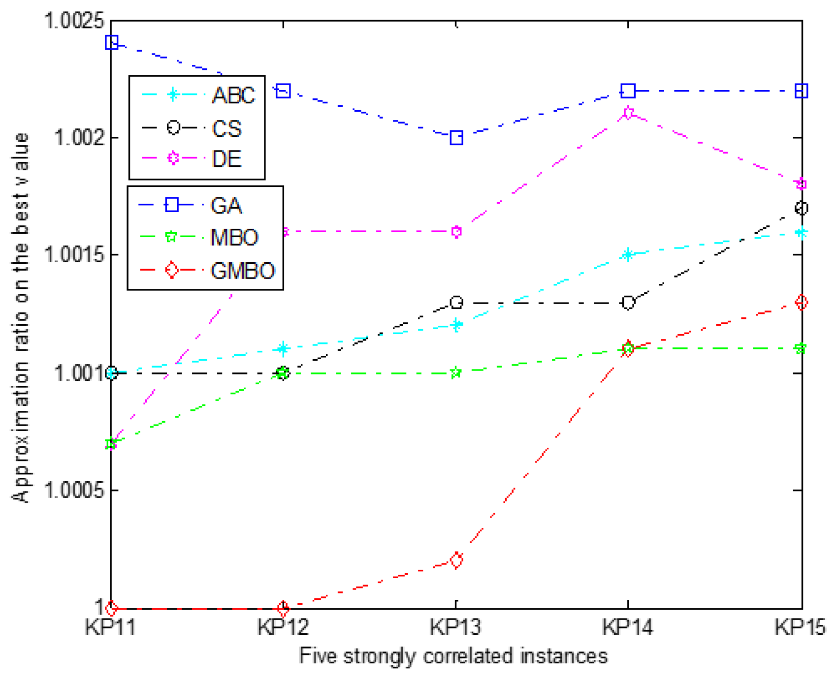
A comparative study of the six methods on five large-scale strongly correlated 0-1 KP instances are recorded in Table 10. Obviously, GMBO outperforms the other five methods for KP11–KP14 on five statistical standards except for Std. ABC obtains the best Std values for KP11–KP15. To KP15, GMBO can get better values on the worst. CS, DE, and GA fail to show outstanding performance for this case. Under these circumstances, the approximation ratio of the worst value of GMBO for KP11–KP15 was less than 1.0019.

For a clearer and more intuitive measure of the similar level of the theoretical optimal value and the actual value obtained by each algorithm, the values of ARB on three types of 0-1 KP instances are illustrated in Figure 4, Figure 5 and Figure 6. From Figure 4, the ARB of GMBO for KP1, KP3, and KP4 were extremely close to or equal to 1. GMBO had the smallest ARB for KP1, KP3–KP5, except for KP2, for which CS obtained the smallest ARB. Similar to Figure 4, from Figure 5, GMBO still had the smallest ARB values, which are 1.0 (KP6, KP7, and KP9) or less than 1.015 (KP8, KP10). In terms of the strongly correlated 0-1 KP instances, GMBO consistently outperformed the other five methods (see Figure 6), in which GMBO had the smallest ARB values except for KP15. Particularly, the ARB of GMBO was even less than 1.0015 for KP15.

Overall, Table 8, Table 9 and Table 10 and Figure 4, Figure 5 and Figure 6 indicate that GMBO was superior to the other five methods when addressing large-scale 0-1 KP problems. In addition, if we look at the worst values achieved by GMBO and the best values obtained by other methods, we can observe that for the majority instances, the former were even far better than the latter.

With regard to the best values, GMBO can gain better values than the others for almost all the instances except KP2, KP5, KP10, and KP15, in which CS and MBO twice achieved the best values, respectively. More specifically, compared to the suboptimal values researched by others, the improvements in KP1–KP15 brought by GMBO were 0.59%, −0.22%, 1.10%, 1.45%, −0.05%, 0.27%, 0.18%, 1.09%, 0.24%, −0.09%, 0.07%, 0.10%, 0.00%, and −0.02%, respectively.

With regard to the mean values, they were very similar to the best values. The improvements in KP1–KP15 were 1.51%, −0.02%, 1.15%, 2.16%, −0.09%, 0.77%, 0.83%, 1.37%, 0.96%, −0.24%, 0.11%, 0.09%, 0.07%, 0.00% and 0.00%, respectively.

With regard to the worst values, GMBO can still reach better values for almost all the 15 instances except KP3, KP5, and KP10 in which MBO was a little better than GMBO. The improvements in KP1–KP15 were 1.73%, 0.23%, −0.29%, 0.80%, −0.17%, 0.94%, 1.00%, 0.37%, 1.05%, −0.44%, 0.10%, 0.02%, 0.00%, 0.00%, and 0.01%, respectively.

In order to test the differences between the proposed GMBO and the other five methods, Wilcoxon’s rank-sum tests with the 5% significance level were used.

Table 11. Rank sum tests for GMBO with the other five methods on KP1–KP15.

GMBO	ABC	CS	DE	GA	MBO
KP1	1	1	1	1	1
KP2	1	1	1	1	0
KP3	1	1	1	1	1
KP4	1	1	1	1	1
KP5	1	1	1	1	−1
KP6	1	1	1	1	1
KP7	1	1	1	1	1
KP8	1	1	1	1	1
KP9	1	1	1	1	1
KP10	1	1	1	1	−1
KP11	1	1	1	1	−1
KP12	1	1	1	1	1
KP13	1	1	1	1	1
KP14	1	1	1	1	0
KP15	1	1	1	1	0
1	15	15	15	15	9
0	0	0	0	0	3
−1	0	0	0	0	3

records the results of rank-sum tests for KP1–KP15. In Table 11, “1” indicates that GMBO outperforms other methods at 95% confidence. Conversely, “−1”. Particularly, “0” represents that the two compared methods possess similar performance. The last three rows summarized the times that GMBO performed better than, similar to, and worse than the corresponding algorithm among 50 runs.

From Table 11, GMBO outperformed ABC, CS, DE, and GA on 15 0-1 KP instances. Compared with MBO, GMBO performed better than, similar to, or worse than MBO on 9, 3, 3 0-1KP instances, respectively. Therefore, one conclusion is easy to draw that GMBO was superior to or at least comparable to the other five methods. This conclusion is consistent with the foregoing analysis.

Table 12. Rankings of six algorithms based on the best values.

	ABC	CS	DE	GA	MBO	GMBO
KP1	4	2	5	6	3	1
KP2	4	1	5	6	2	3
KP3	4	3	5	6	2	1
KP4	4	2	5	6	3	1
KP5	3	4	5	6	1	2
KP6	4	2	5	6	3	1
KP7	4	2	5	6	3	1
KP8	4	2	5	6	3	1
KP9	4	2	5	6	3	1
KP10	4	1	5	6	3	2
KP11	4	4	2	6	2	1
KP12	4	2	5	6	2	1
KP13	3	4	5	6	2	1
KP14	4	3	5	6	2	1
KP15	3	4	5	6	1	2
Mean rank	3.80	2.53	4.80	6	2.33	1.33

,

Table 13. Rankings of six algorithms based on the mean values.

	ABC	CS	DE	GA	MBO	GMBO
KP1	3	4	5	6	2	1
KP2	3	4	5	6	1	2
KP3	3	4	5	6	2	1
KP4	3	4	5	6	2	1
KP5	3	4	5	6	1	2
KP6	4	3	5	6	2	1
KP7	4	3	5	6	2	1
KP8	3	4	5	6	2	1
KP9	4	3	5	6	2	1
KP10	3	4	5	6	1	2
KP11	4	5	3	6	2	1
KP12	3	4	5	6	2	1
KP13	3	4	5	6	2	1
KP14	3	4	5	6	2	1
KP15	3	4	5	6	1	2
Mean rank	3.27	3.87	4.87	6	1.73	1.27

and

Table 14. Rankings of six algorithms based on the worst values.

	ABC	CS	DE	GA	MBO	GMBO
KP1	3	4	5	6	2	1
KP2	3	4	5	6	2	1
KP3	3	4	5	6	1	2
KP4	3	4	5	6	2	1
KP5	3	4	5	6	1	2
KP6	3	4	5	6	2	1
KP7	3	4	5	6	2	1
KP8	3	4	5	6	2	1
KP9	3	4	5	6	2	1
KP10	3	4	5	6	1	2
KP11	2	4	5	6	3	1
KP12	2	4	5	6	2	1
KP13	1	4	5	6	3	1
KP14	1	3	5	6	4	1
KP15	3	4	5	6	2	1
Mean rank	2.60	3.93	5	6	2.07	1.20

illustrate the ranks of six methods for 15 large-scale 0-1 KP instances on the best values, the mean values, and the worst values, respectively. These clearly show the performance of GMBO in comparison with the other five algorithms.

According to Table 12, obviously, the proposed GMBO exhibited superior performance compared with all the other five methods. In addition, CS and MBO can be regarded as the second-best methods, having identical performance. GA consistently showed the worst performance. Overall, the average rank in descending order according to the best values were: GMBO (1.33), MBO (2.33), CS (2.53), ABC (3.80), DE (4.80), and GA (6).

From Table 13, we can see that the average rank of GMBO still occupied the first. MBO consistently outperformed the other four methods. Note that the rank value of ABC was identical to that of CS. The detailed rank was as follows: GMBO (1.27), MBO (1.73), ABC (3.27), CS (3.87), DE (4.87), and GA (6).

Table 14 shows the statistical results of the six methods based on the worst values. The ranking order of the six methods was GMBO (1.20), MBO (2.07), ABC (2.60), CS (3.93), DE (5), and GA (6), which was identical with that in Table 12.

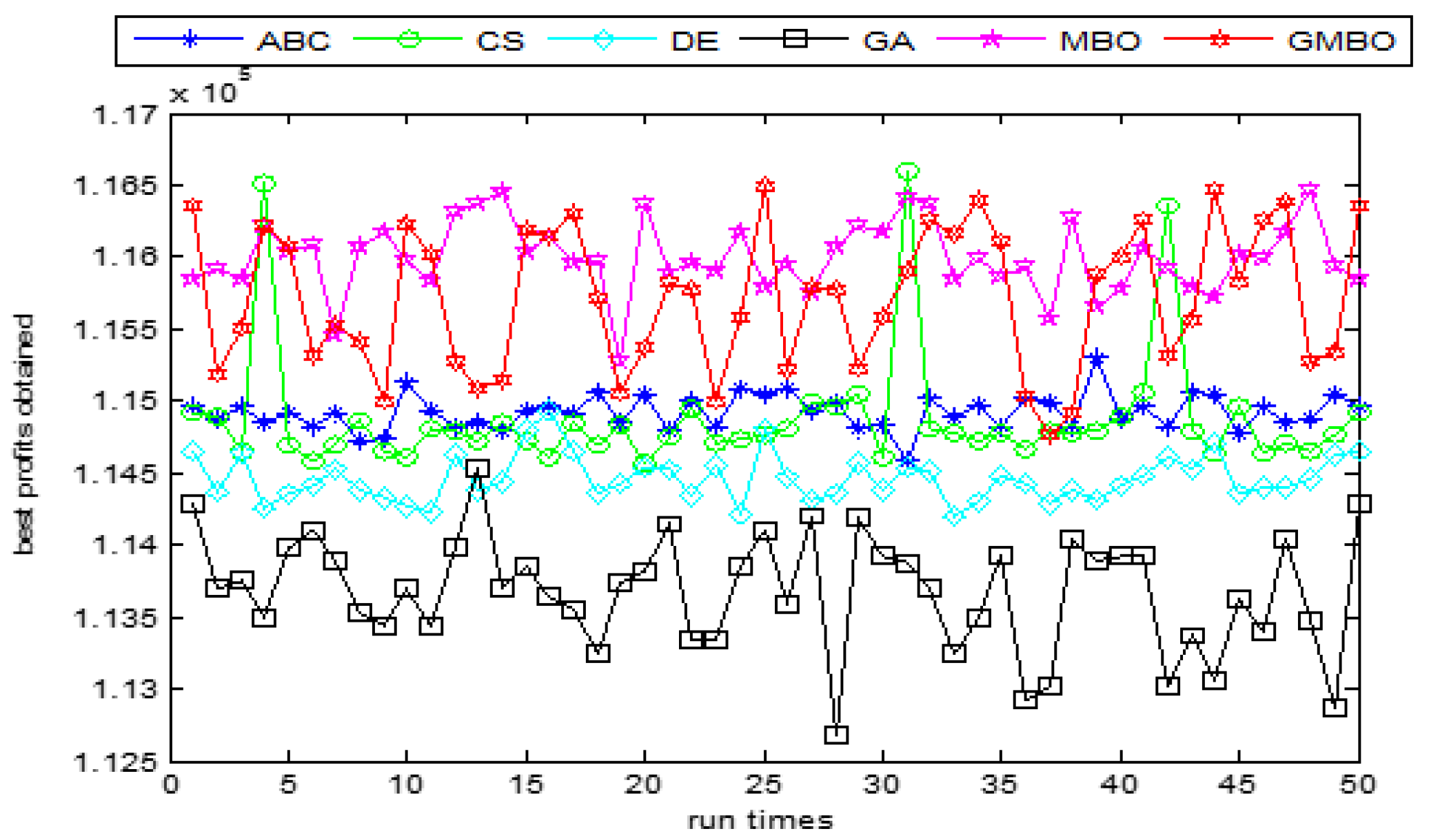
Then, a comparison of the six highest dimensional 0-1 KP instances, i.e., KP4, KP5, KP9, KP10, KP14, and KP15, is illustrated in Figure 7, Figure 8, Figure 9, Figure 10, Figure 11 and Figure 12, which was based on the best profits achieved by 50 runs.

Figure 7, Figure 9 and Figure 11 illustrate the best values achieved by the six methods on 1500-dimensional uncorrelated, weakly correlated, and strongly correlated 0-1 KP instances in 50 runs, respectively. From Figure 7, it can be easily seen that the best values obtained by GMBO far exceed that of the other five methods. Meanwhile, the two best values of CS outstripped the two worst values of GMBO. By looking at Figure 9, we can conclude that GMBO greatly outperformed the other five methods. The distribution of best values of GMBO in 50 times was close to a horizontal line, which pointed towards the excellent stability of GMBO in this case. With regard to numerical stability, CS had the worst performance. From Figure 11, the curve of GMBO still overtopped that of ABC, CS, DE, and GA, as illustrated in Figure 7 and Figure 9. This advantage, however, was not obvious when compared with MBO.

Figure 8, Figure 10 and Figure 12 show the best values obtained by six methods on 2000-dimensional uncorrelated, weakly correlated, and strongly correlated 0-1 KP instances in 50 runs, respectively. As the dimension becomes large, space is expanded dramatically to 2²⁰⁰⁰, which represents a challenge for any method. It can be said with certainty that almost all the values of GMBO are bigger than that of the other five methods except MBO. Similar to Figure 11, the curves of MBO partially overlaps that of GMBO in Figure 12, which may be interpreted as the ability of GMBO towards competing with MBO.

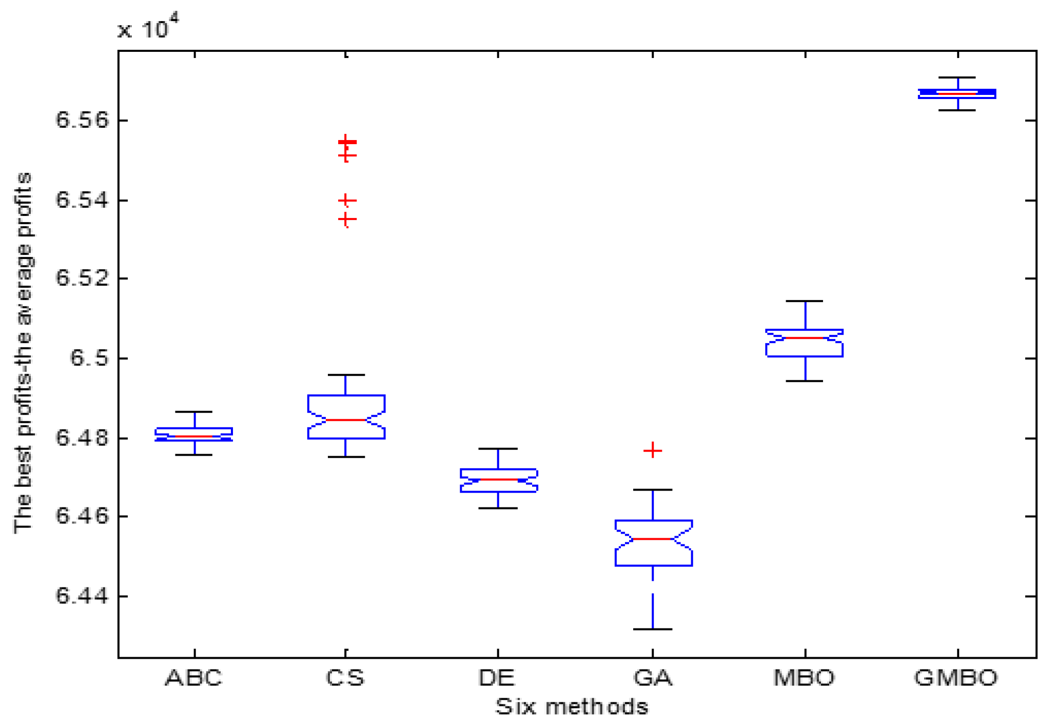
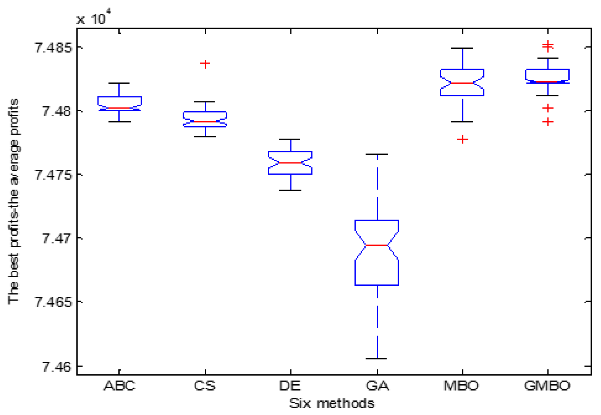
For the purpose of visualizing the experimental results from the statistical perspective, the corresponding boxplots of six higher dimensional KP4–KP5, KP9–KP10, and KP14-15 are shown in Figure 13, Figure 14, Figure 15, Figure 16, Figure 17 and Figure 18. On the whole, the boxplot for GMBO has greater value and less height than those of the other five methods, which indicates the stronger optimization ability and stability of GMBO even encountering high-dimensional instances.

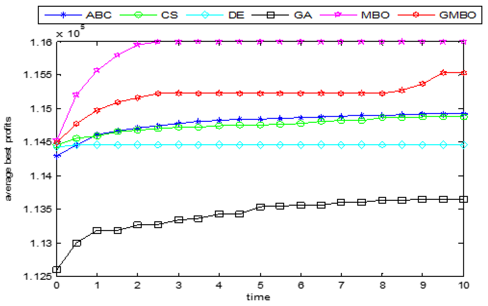
In order to examine the convergence rate of GMBO, the evolutionary process and convergent trajectories of six methods are illustrated in Figure 19, Figure 20, Figure 21, Figure 22, Figure 23 and Figure 24. It should be noted that six high dimensional instances, viz., KP4, KP5, KP9, KP10, KP14, and KP15, were chosen. In addition, Figure 19, Figure 20, Figure 21, Figure 22, Figure 23 and Figure 24 show the average best values with 50 runs, and not one independent experimental result.

From Figure 19, the curves of GMBO and MBO were almost coincident before 6 s, but afterward, GMBO converged rapidly to a better value as compared to the others. From Figure 20, it is indeed interesting to note that MBO has a weak advantage in the average values as compared to GMBO. From Figure 21, MBO and GMBO have identical initial function values, and the average values obtained by MBO were better than that of GMBO before 3 s. However, similar to the trend in Figure 19, 3 s later, GMBO quickly converged to a higher value. As depicted in Figure 22, unexpectedly, when addressing the 2000-dimensional weakly correlated 0-1 KP instances, GMBO was inferior to MBO. Figure 23 and Figure 24 illustrate the evolutionary process of strongly correlated 0-1 KP instances. By observation of 2 convergence graphs, we can conclude that GMBO and MBO have similar performance. Throughout Figure 19, Figure 20, Figure 21, Figure 22, Figure 23 and Figure 24, GMBO has a stronger optimization ability and faster convergence speed to reach optimum solutions than the other five methods.

4.4. The Comparisons of the GMBO and the Latest Algorithms

To evaluate the performance of the proposed GMBO, the two latest algorithms, namely, moth search (MS) [67] and moth-flame optimization (MFO) [68], were especially selected to compare with GMBO. The following factors were mainly considered. (1) The literature on the application of MS and MFO to solve 0-1 KP problem was not found. (2) The GMBO, MS, and MFO were novel nature-inspired swarm intelligence algorithms, which simulated the migration behavior of the monarch butterfly, the Lévy flight mode, or the navigation method of moths.

For MS, the max step S_max = 1.0, acceleration factor $\phi$ = 0.618, and the index $\beta$ = 1.5. For MFO, the maximum number of flames N = 30. In order to make a fair comparison, all experiments were conducted in the same experimental environment as described above. The detailed experimental results of GMBO and the other two algorithms on the three kinds of large-scale 0-1 KP instances were presented in

Table 15. Performance comparison of three algorithms on large-scale 0-1 KP instances.

No.	MBO			MFO			MS
	Best	Mean	Std	Best	Mean	Std	Best	Mean	Std
KP1	40,684	40,641	40.09	40,538	39,976	309.00	40,242	40,101	56.37
KP2	49,992	49,732	116.12	50590	50200	384.72	50,056	49,790	79.57
KP3	61764	61430	379.76	61,836	61,238	608.78	61,059	60,721	101.80
KP4	76,929	76,691	267.90	77,007	76,353	656.36	75,716	75,505	95.94
KP5	99,898	99,424	200.38	102,276	101,475	781.66	100,348	100,036	120.08
KP6	35,069	35,064	4.04	35,069	34,952	116.84	34,850	34,799	20.64
KP7	43,786	43,784	1.57	43,784	43,630	132.21	43,474	43,424	20.34
KP8	53,426	53,167	300.90	53,552	53,048	556.60	52,637	52,489	73.73
KP9	65,708	65,666	18.48	65,692	65,421	253.29	65,093	65,025	27.59
KP10	116,496	115,718	492.92	118,183	117,381	838.07	116,283	115,937	117.92
KP11	40,167	40,162	5.11	40,157	40,142	15.48	40,137	40,127	5.58
KP12	49,442	49,425	11.58	49,433	49,411	15.64	49,403	49,390	7.10
KP13	60,630	60,604	20.88	60,581	60,557	68.28	60,581	60,571	9.24
KP14	74,852	74,852	12.00	74,910	74,874	32.49	74,852	74,833	7.71
KP15	99,553	99,534	14.14	99,643	99,602	37.10	99,572	99,546	9.28
Total	8	10	5	8	5	0	0	0	10

. The best, mean, and standard deviation values in bold indicate superiority. The dominant times of the three algorithms in the three statistical values are given in the last line of Table 15. As the results presented in Table 15, the number of times the GMBO algorithm had priority in the best, the mean, and the standard deviation values were 8, 10, 5, respectively. The simulation results indicated that GMBO generally provided very excellent performance in most instances compared with MFO and MS. The two metrics, namely mean and standard deviation, demonstrated again that GMBO was more stable. The comprehensive performance of MFO was superior to that of MS.

To summarize, by analyzing Table 4, Table 5, Table 6, Table 7, Table 8, Table 9, Table 10, Table 11, Table 12, Table 13, Table 14 and Table 15 and Figure 4, Figure 5, Figure 6, Figure 7, Figure 8, Figure 9, Figure 10, Figure 11, Figure 12, Figure 13, Figure 14, Figure 15, Figure 16, Figure 17, Figure 18, Figure 19, Figure 20, Figure 21, Figure 22, Figure 23 and Figure 24, it can be inferred that GMBO had better optimization capability, numerical stability, and higher convergence speed. In other words, it can be claimed that GMBO is an excellent MBO variant, which is capable of addressing large-scale 0-1 KP instances.

5. Conclusions

In order to tackle high-dimensional 0-1 KP problems more efficiently and effectively, as well as to overcome the shortcomings of the original MBO simultaneously, a novel monarch butterfly optimization with the global position updating operator (GMBO) has been proposed in this manuscript. Firstly, a simple and effective dichotomy encoding scheme, without changing the evolutionary formula, is used. Moreover, an ingenious global position updating operator is introduced with the intention of enhancing the optimization capacity and convergence speed. The inspiration behind the new operator lies in creating a balance between intensification and diversification, a very important feature in the field of metaheuristics. Furthermore, a two-stage individual optimization method based on the greedy strategy is employed, which besides guaranteeing the feasibility of the solutions, is able to improve the quality further. In addition, the Orthogonal Design (OD) was applied to find suitable parameters. Finally, GMBO was verified and compared with ABC, CS, DE, GA, and MBO on large-scale 0-1 KP instances. The experimental results demonstrate that GMBO outperforms the other five algorithms on solution precision, convergence speed, and numerical stability.

The introduction of a global position operator coupled with an efficient two-stage repairing operator is instrumental towards the superior performance of GMBO. However, there is room for further enhancing the performance of GMBO. Firstly, the hybridization of the two methods complementing each other is becoming more and more popular, such as the hybridization of HS with CS [69]. Combining MBO with other methods could indeed be very promising and hence worth experimentation. Secondly, in the present work, three groups of high-dimensional 0-1 KP instances were selected. In the future, a multidimensional knapsack problem, quadratic knapsack problem, knapsack sharing problem, and randomized time-varying knapsack problem can be considered to investigate the performance of MBO. Thirdly, some typical combinatorial optimization problems, such as job scheduling problems [70,71,72], feature selection [73,74,75], and classification [76], deserve serious investigation and discussion. For these challenging engineering problems, the key issue is how to encode and process constraints. The application of MBO for these problems is another interesting research area. Finally, perturb [77], ensemble [78], learning mechanisms [79,80], or information feedback mechanisms [81] can be effectively combined with MBO to improve performance.

References

- Martello, S.; Toth, P. Knapsack Problems: Algorithms and Computer Implementations; John Wiley & Sons, Inc.: Hoboken, NJ, USA, 1990. [Google Scholar]
- Mavrotas, G.; Diakoulaki, D.; Kourentzis, A. Selection among ranked projects under segmentation, policy and logical constraints. Eur. J. Oper. Res. 2008, 187, 177–192. [Google Scholar] [CrossRef]
- Peeta, S.; Salman, F.S.; Gunnec, D.; Viswanath, K. Pre-disaster investment decisions for strengthening a highway network. Comput. Oper. Res. 2010, 37, 1708–1719. [Google Scholar] [CrossRef]
- Yates, J.; Lakshmanan, K. A constrained binary knapsack approximation for shortest path network interdiction. Comput. Ind. Eng. 2011, 61, 981–992. [Google Scholar] [CrossRef]
- Dantzig, G.B. Discrete-variable extremum problems. Oper. Res. 1957, 5, 266–288. [Google Scholar] [CrossRef]
- Shih, W. A branch and bound method for the multi-constraint zero-one knapsack problem. J. Oper. Res. Soc. 1979, 30, 369–378. [Google Scholar] [CrossRef]
- Toth, P. Dynamic programing algorithms for the zero-one knapsack problem. Computing 1980, 25, 29–45. [Google Scholar] [CrossRef]
- Martello, S.; Toth, P. A new algorithm for the 0-1 knapsack problem. Manag. Sci. 1988, 34, 633–644. [Google Scholar] [CrossRef]
- Pisinger, D. An expanding-core algorithm for the exact 0–1 knapsack problem. Eur. J. Oper. Res. 1995, 87, 175–187. [Google Scholar] [CrossRef]
- Puchinger, J.; Raidl, G.R.; Pferschy, U. The Core Concept for the Multidimensional Knapsack Problem. In Proceedings of the European Conference on Evolutionary Computation in Combinatorial Optimization, Budapest, Hungary, 10–12 April 2006; Gottlieb, J., Raidl, G.R., Eds.; Springer: Berlin, Germany, 2006; pp. 195–208. [Google Scholar] [Green Version]
- Thiel, J.; Voss, S. Some experiences on solving multi constraint zero-one knapsack problems with genetic algorithms. Inf. Syst. Oper. Res. 1994, 32, 226–242. [Google Scholar]
- Chen, P.; Li, J.; Liu, Z.M. Solving 0-1 knapsack problems by a discrete binary version of differential evolution. In Proceedings of the Second International Symposium on Intelligent Information Technology Application, Shanghai, China, 21–22 December 2008; Volume 2, pp. 513–516. [Google Scholar]
- Bhattacharjee, K.K.; Sarmah, S.P. Shuffled frog leaping algorithm and its application to 0/1 knapsack problem. Appl. Soft Comput. 2014, 19, 252–263. [Google Scholar] [CrossRef]
- Feng, Y.H.; Jia, K.; He, Y.C. An improved hybrid encoding cuckoo search algorithm for 0-1 knapsack problems. Comput. Intell. Neurosci. 2014, 2014, 1. [Google Scholar] [CrossRef]
- Feng, Y.H.; Wang, G.G.; Feng, Q.J.; Zhao, X.J. An effective hybrid cuckoo search algorithm with improved shuffled frog leaping algorithm for 0-1 knapsack problems. Comput. Intell. Neurosci. 2014, 2014, 36. [Google Scholar] [CrossRef]
- Kashan, M.H.; Nahavandi, N.; Kashan, A.H. DisABC: A new artificial bee colony algorithm for binary optimization. Appl. Soft Comput. 2012, 12, 342–352. [Google Scholar] [CrossRef]
- Xue, Y.; Jiang, J.; Zhao, B.; Ma, T. A self-adaptive artificial bee colony algorithm based on global best for global optimization. Soft Comput. 2018, 22, 2935–2952. [Google Scholar] [CrossRef]
- Zong, W.G.; Kim, J.H.; Loganathan, G.V. A New Heuristic Optimization Algorithm: Harmony Search. Simulation 2001, 76, 60–68. [Google Scholar] [CrossRef]
- Zou, D.; Gao, L.; Li, S.; Wu, J. Solving 0-1 knapsack problem by a novel global harmony search algorithm. Appl. Soft Comput. 2011, 11, 1556–1564. [Google Scholar] [CrossRef]
- Kong, X.; Gao, L.; Ouyang, H.; Li, S. A simplified binary harmony search algorithm for large scale 0-1 knapsack problems. Expert Syst. Appl. 2015, 42, 5337–5355. [Google Scholar] [CrossRef]
- Rezoug, A.; Boughaci, D. A self-adaptive harmony search combined with a stochastic local search for the 0-1 multidimensional knapsack problem. Int. J. Biol. Inspir. Comput. 2016, 8, 234–239. [Google Scholar] [CrossRef]
- Zhou, Y.; Li, L.; Ma, M. A complex-valued encoding bat algorithm for solving 0-1 knapsack problem. Neural Process. Lett. 2016, 44, 407–430. [Google Scholar] [CrossRef]
- Cai, X.; Gao, X.-Z.; Xue, Y. Improved bat algorithm with optimal forage strategy and random disturbance strategy. Int. J. Biol. Inspir. Comput. 2016, 8, 205–214. [Google Scholar] [CrossRef]
- Zhang, X.; Huang, S.; Hu, Y.; Zhang, Y.; Mahadevan, S.; Deng, Y. Solving 0-1 knapsack problems based on amoeboid organism algorithm. Appl. Math. Comput. 2013, 219, 9959–9970. [Google Scholar] [CrossRef]
- Li, X.; Zhang, J.; Yin, M. Animal migration optimization: An optimization algorithm inspired by animal migration behavior. Neural Comput. Appl. 2014, 24, 1867–1877. [Google Scholar] [CrossRef]
- Cui, Z.; Fan, S.; Zeng, J.; Shi, Z. Artificial plant optimization algorithm with three-period photosynthesis. Int. J. Biol. Inspir. Comput. 2013, 5, 133–139. [Google Scholar] [CrossRef]
- Simon, D. Biogeography-based optimization. IEEE Trans. Evol. Comput. 2008, 12, 702–713. [Google Scholar] [CrossRef]
- Li, X.; Wang, J.; Zhou, J.; Yin, M. A perturb biogeography based optimization with mutation for global numerical optimization. Appl. Math. Comput. 2011, 218, 598–609. [Google Scholar] [CrossRef]
- Wang, L.; Yang, R.; Ni, H.; Ye, W.; Fei, M.; Pardalos, P.M. A human learning optimization algorithm and its application to multi-dimensional knapsack problems. Appl. Soft Comput. 2015, 34, 736–743. [Google Scholar] [CrossRef]
- Wang, G.-G.; Guo, L.H.; Wang, H.Q.; Duan, H.; Liu, L.; Li, J. Incorporating mutation scheme into krill herd algorithm for global numerical optimization. Neural Comput. Appl. 2014, 24, 853–871. [Google Scholar] [CrossRef]
- Wang, G.-G.; Gandomi, A.H.; Yang, X.-S.; Alavi, H.A. A new hybrid method based on krill herd and cuckoo search for global optimization tasks. Int. J. Biol. Inspir. Comput. 2016, 8, 286–299. [Google Scholar] [CrossRef]
- Wang, G.-G.; Gandomi, A.H.; Alavi, H.A. Stud krill herd algorithm. Neurocomputing 2014, 128, 363–370. [Google Scholar] [CrossRef]
- Wang, G.-G.; Deb, S.; Cui, Z. Monarch butterfly optimization. Neural Comput. Appl. 2015. [Google Scholar] [CrossRef]
- Wang, G.-G.; Deb, S.; Gao, X.-Z.; Coelho, L.D.S. A new metaheuristic optimization algorithm motivated by elephant herding behavior. Int. J. Biol. Inspir. Comput. 2016, 8, 394–409. [Google Scholar] [CrossRef]
- Sang, H.-Y.; Duan, Y.P.; Li, J.-Q. An effective invasive weed optimization algorithm for scheduling semiconductor final testing problem. Swarm Evol. Comput. 2018, 38, 42–53. [Google Scholar] [CrossRef]
- Wang, G.-G.; Deb, S.; Coelho, L.D.S. Earthworm optimisation algorithm: A bio-inspired metaheuristic algorithm for global optimisation problems. Int. J. Biol. Inspir. Comput. 2018, 12, 1–22. [Google Scholar] [CrossRef]
- Jain, M.; Singh, V.; Rani, A. A novel nature-inspired algorithm for optimization: Squirrel search algorithm. Swarm Evol. Comput. 2019, 44, 148–175. [Google Scholar] [CrossRef]
- Singh, B.; Anand, P. A novel adaptive butterfly optimization algorithm. Int. J. Comput. Mater. Sci. Eng. 2018, 7, 69–72. [Google Scholar] [CrossRef]
- Sayed, G.I.; Khoriba, G.; Haggag, M.H. A novel chaotic salp swarm algorithm for global optimization and feature selection. Appl. Intell. 2018, 48, 3462–3481. [Google Scholar] [CrossRef]
- Simhadri, K.S.; Mohanty, B. Performance analysis of dual-mode PI controller using quasi-oppositional whale optimization algorithm for load frequency control. Int. Trans. Electr. Energy Syst. 2019. [Google Scholar] [CrossRef]
- Brezočnik, L.; Fister, I.; Podgorelec, V. Swarm intelligence algorithms for feature selection: A review. Appl. Sci. 2018, 8, 1521. [Google Scholar] [CrossRef]
- Feng, Y.H.; Wang, G.-G.; Deb, S.; Lu, M.; Zhao, X.-J. Solving 0-1 knapsack problem by a novel binary monarch butterfly optimization. Neural Comput. Appl. 2015. [Google Scholar] [CrossRef]
- Wang, G.-G.; Zhao, X.C.; Deb, S. A Novel Monarch Butterfly Optimization with Greedy Strategy and Self-adaptive Crossover Operator. In Proceedings of the 2nd International Conference on Soft Computing & Machine Intelligence (ISCMI 2015), Hong Kong, China, 23–24 November 2015. [Google Scholar]
- He, Y.C.; Wang, X.Z.; Kou, Y.Z. A binary differential evolution algorithm with hybrid encoding. J. Comput. Res. Dev. 2007, 44, 1476–1484. [Google Scholar] [CrossRef]
- He, Y.C.; Song, J.M.; Zhang, J.M.; Gou, H.Y. Research on genetic algorithms for solving static and dynamic knapsack problems. Appl. Res. Comput. 2015, 32, 1011–1015. [Google Scholar]
- He, Y.C.; Zhang, X.L.; Li, W.B.; Li, X.; Wu, W.L.; Gao, S.G. Algorithms for randomized time-varying knapsack problems. J. Comb. Optim. 2016, 31, 95–117. [Google Scholar] [CrossRef]
- Fang, K.-T.; Wang, Y. Number-Theoretic Methods in Statistics; Chapman & Hall: New York, NY, USA, 1994. [Google Scholar]
- Wilcoxon, F.; Katti, S.K.; Wilcox, R.A. Critical values and probability levels for the Wilcoxon rank sum test and the Wilcoxon signed rank test. Sel. Tables Math. Stat. 1970, 1, 171–259. [Google Scholar]
- Gutowski, M. Lévy flights as an underlying mechanism for global optimization algorithms. arXiv 2001, arXiv:math-ph/0106003. [Google Scholar]
- Pavlyukevich, I. Levy flights, non-local search and simulated annealing. Mathematics 2007, 226, 1830–1844. [Google Scholar] [CrossRef]
- Kennedy, J.; Eberhart, R.C. A discrete binary version of the particle swarm algorithm. In Proceedings of the 1997 Conference on Systems, Man, and Cybernetics, Orlando, FL, USA, 12–15 October 1997; pp. 4104–4108. [Google Scholar]
- Zhu, H.; He, Y.; Wang, X.; Tsang, E.C. Discrete differential evolutions for the discounted {0-1} knapsack problem. Int. J. Biol. Inspir. Comput. 2017, 10, 219–238. [Google Scholar] [CrossRef]
- Yang, X.S.; Deb, S.; Hanne, T.; He, X. Attraction and Diffusion in Nature-Inspired Optimization Algorithms. Neural Comput. Appl. 2019, 31, 1987–1994. [Google Scholar] [CrossRef]
- Joines, J.A.; Houck, C.R. On the use of non-stationary penalty functions to solve nonlinear constrained optimization problems with GA’s. Evolutionary Computation. In Proceedings of the First IEEE Conference on Evolutionary Computation, Orlando, FL, USA, 27–29 June 1994; pp. 579–584. [Google Scholar]
- Olsen, A.L. Penalty functions and the knapsack problem. Evolutionary Computation. In Proceedings of the First IEEE Conference on Evolutionary Computation, Orlando, FL, USA, 27–29 June 1994; pp. 554–558. [Google Scholar]
- Goldberg, D.E. Genetic Algorithms in Search, Optimization, and Machine Learning; Addison-Wesley: Boston, MA, USA, 1989. [Google Scholar]
- Simon, D. Evolutionary Optimization Algorithms; Wiley: New York, NY, USA, 2013. [Google Scholar]
- Du, D.Z.; Ko, K.I.; Hu, X. Design and Analysis of Approximation Algorithms; Springer Science & Business Media: Berlin, Germany, 2011. [Google Scholar]
- Pisinger, D. Where are the hard knapsack problems. Comput. Oper. Res. 2005, 32, 2271–2284. [Google Scholar] [CrossRef]
- Karaboga, D.; Basturk, B. A powerful and efficient algorithm for numerical function optimization: Artificial bee colony (ABC) algorithm. J. Glob. Optim. 2007, 39, 459–471. [Google Scholar] [CrossRef]
- Yang, X.S.; Deb, S. Cuckoo search via Lévy flights. In Proceedings of the World Congress on Nature and Biologically Inspired Computing (NaBIC 2009), Coimbatore, India, 9–11 December 2009; pp. 210–214. [Google Scholar]
- Storn, R.; Price, K. Differential evolution–A simple and efficient heuristic for global optimization over continuous spaces. J. Glob. Optim. 1997, 11, 341–359. [Google Scholar] [CrossRef]
- Mahdavi, M.; Fesanghary, M.; Damangir, E. An improved harmony search algorithm for solving optimization problems. Appl. Math. Comput. 2007, 188, 1567–1579. [Google Scholar] [CrossRef]
- Bansal, J.C.; Deep, K. A Modified Binary Particle Swarm Optimization for Knapsack Problems. Appl. Math. Comput. 2012, 218, 11042–11061. [Google Scholar] [CrossRef]
- Lee, C.Y.; Lee, Z.J.; Su, S.F. A New Approach for Solving 0/1 Knapsack Problem. In Proceedings of the IEEE International Conference on Systems, Man and Cybernetics, Montreal, QC, Canada, 7–10 October 2007; pp. 3138–3143. [Google Scholar]
- Cormen, T.H. Introduction to Algorithms; MIT Press: Cambridge, MA, USA, 2009. [Google Scholar]
- Wang, G.-G. Moth search algorithm: A bio-inspired metaheuristic algorithm for global optimization problems. Memet. Comput. 2018, 10, 151–164. [Google Scholar] [CrossRef]
- Mehne, S.H.H.; Mirjalili, S. Moth-Flame Optimization Algorithm: Theory, Literature Review, and Application in Optimal Nonlinear. In Nature Inspired Optimizers: Theories, Literature Reviews and Applications; Mirjalili, S., Jin, S.D., Lewis, A., Eds.; Spring: Berlin, Germany, 2020; Volume 811, p. 143. [Google Scholar]
- Gandomi, A.H.; Zhao, X.J.; Chu, H.C.E. Hybridizing harmony search algorithm with cuckoo search for global numerical optimization. Soft Comput. 2016, 20, 273–285. [Google Scholar]
- Li, J.-Q.; Pan, Q.-K.; Liang, Y.-C. An effective hybrid tabu search algorithm for multi-objective flexible job-shop scheduling problems. Comput. Ind. Eng. 2010, 59, 647–662. [Google Scholar] [CrossRef]
- Han, Y.-Y.; Gong, D.; Sun, X. A discrete artificial bee colony algorithm incorporating differential evolution for the flow-shop scheduling problem with blocking. Eng. Optim. 2014, 47, 927–946. [Google Scholar] [CrossRef]
- Li, J.-Q.; Pan, Q.-K.; Tasgetiren, M.F. A discrete artificial bee colony algorithm for the multi-objective flexible job-shop scheduling problem with maintenance activities. Appl. Math. Model. 2014, 38, 1111–1132. [Google Scholar] [CrossRef]
- Zhang, W.-Q.; Zhang, Y.; Peng, C. Brain storm optimization for feature selection using new individual clustering and updating mechanism. Appl. Intell. 2019. [Google Scholar] [CrossRef]
- Zhang, Y.; Li, H.-G.; Wang, Q.; Peng, C. A filter-based bare-bone particle swarm optimization algorithm for unsupervised feature selection. Appl. Intell. 2019, 49, 2889–2898. [Google Scholar] [CrossRef]
- Zhang, Y.; Wang, Q.; Gong, D.-W.; Song, X.-F. Nonnegative laplacian embedding guided subspace learning for unsupervised feature selection. Pattern Recognit. 2019, 93, 337–352. [Google Scholar] [CrossRef]
- Zhang, Y.; Gong, D.W.; Cheng, J. Multi-objective particle swarm optimization approach for cost-based feature selection in classification. IEEE ACM Trans. Comput. Biol. Bioinform. 2017, 14, 64–75. [Google Scholar] [CrossRef]
- Zhao, X. A perturbed particle swarm algorithm for numerical optimization. Appl. Soft Comput. 2010, 10, 119–124. [Google Scholar]
- Wu, G.; Shen, X.; Li, H.; Chen, H.; Lin, A.; Suganthan, P.N. Ensemble of differential evolution variants. Inf. Sci. 2018, 423, 172–186. [Google Scholar] [CrossRef]
- Wang, G.G.; Deb, S.; Gandomi, A.H.; Alavi, A.H. Opposition-based krill herd algorithm with Cauchy mutation and position clamping. Neurocomputing 2016, 177, 147–157. [Google Scholar] [CrossRef]
- Zhang, Y.; Gong, D.-W.; Gao, X.-Z.; Tian, T.; Sun, X.-Y. Binary differential evolution with self-learning for multi-objective feature selection. Inf. Sci. 2020, 507, 67–85. [Google Scholar] [CrossRef]
- Wang, G.-G.; Tan, Y. Improving metaheuristic algorithms with information feedback models. IEEE Trans. Cybern. 2019, 49, 542–555. [Google Scholar] [CrossRef]
Figure 1.
The example of the dichotomy encoding scheme.
Figure 2.
Flowchart of global position updating operator (GMBO) algorithm for 0-1 knapsack (KP) problem.
Figure 3.
The changing trends of all the factor levels.
Figure 4.
Comparison of ARB for KP1-KP5.
Figure 5.
Comparison of ARB for KP6-KP10.
Figure 6.
Comparison of ARB for KP11-KP15.
Figure 7.
Comparison of the best values on KP4 in 50 runs.
Figure 8.
Comparison of the best values on KP5 in 50 runs.
Figure 9.
Comparison of the best values on KP9 in 50 runs.
Figure 10.
Comparison of the best values on KP10 in 50 runs.
Figure 11.
Comparison of the best values on KP14 in 50 runs.
Figure 12.
Comparison of the best values on KP15 in 50 runs.
Figure 13.
Boxplot of the best values on KP4 in 50 runs.
Figure 14.
Boxplot of the best values on KP5 in 50 runs.
Figure 15.
Boxplot of the best values on KP9 in 50 runs.
Figure 16.
Boxplot of the best values on KP10 in 50 runs.
Figure 17.
Boxplot of the best values on KP14 in 50 runs.
Figure 18.
Boxplot of the best values on KP15 in 50 runs.
Figure 19.
The convergence graph of six methods on KP4 in 10 s.
Figure 20.
The convergence graph of six methods on KP5 in 10 s.
Figure 21.
The convergence graph of six methods on KP9 in 10 s.
Figure 22.
The convergence graph of six methods on KP10 in 10 s.
Figure 23.
The convergence graph of six methods on KP14 in 10 s.
Figure 24.
The convergence graph of six methods on KP15 in 10 s.