Econophysics and Fractional Calculus: Einstein’s Evolution Equation, the Fractal Market Hypothesis, Trend Analysis and Future Price Prediction

Abstract

This paper examines a range of results that can be derived from Einstein’s evolution equation focusing on the effect of introducing a Lévy distribution into the evolution equation. In this context, we examine the derivation (derived exclusively from the evolution equation) of the classical and fractional diffusion equations, the classical and generalised Kolmogorov–Feller equations, the evolution of self-affine stochastic fields through the fractional diffusion equation, the fractional Poisson equation (for the time independent case), and, a derivation of the Lyapunov exponent and volatility. In this way, we provide a collection of results (which includes the derivation of certain fractional partial differential equations) that are fundamental to the stochastic modelling associated with elastic scattering problems obtained under a unifying theme, i.e., Einstein’s evolution equation. This includes an analysis of stochastic fields governed by a symmetric (zero-mean) Gaussian distribution, a Lévy distribution characterised by the Lévy index $\gamma \in [0,2]$ and the derivation of two impulse response functions for each case. The relationship between non-Gaussian distributions and fractional calculus is examined and applications to financial forecasting under the fractal market hypothesis considered, the reader being provided with example software functions (written in MATLAB) so that the results presented may be reproduced and/or further investigated.

1. Introduction

We study one of the principal field equations in statistical mechanics, namely, Einstein’s evolution equation (EEE or E${}^3$). This is done in order to derive mathematical models and thereby specific financial indices in a unified manner, an approach which includes the use of fractional calculus.

E${}^3$ models the random motion and (elastic) interactions of a canonical ensemble of particles. It provides a description for the time evolution of the spatial density field that represents the concentration of such particles in a macroscopic sense. In an n-dimensional space, each particle is taken to be undergoing a random walk in which the direction that a particle “propagates” after a “scattering event” (in which energy and momentum are conserved) is random together with the length of propagation. The scattering angle $\theta$ is taken to be conform to a distribution of angles $\mathrm{Pr}\left[\theta \left(\mathbf{r}\right)\right],\mathbf{r}\in {\mathbb{R}}^n$ and the (free) propagation length is taken to conform to some distribution of lengths $\mathrm{Pr}\left[L\right(\mathbf{r}\left)\right]$ whose mean value defines the mean free path (MFP). This was the basis for Albert Einstein’s original study of Brownian motion in 1905 [1], albeit for the one-dimensional case.

In addition to the work of Josiah Gibbs, the evolution equation that Einstein derived is one the foundations of statistical mechanics [2,3]. The approach can, for example, be applied equally well to modelling the diffusion of light propagating through a complex of scatterers. In this case the light is taken to be a ray-field where each ray (reflected from one particle to another) has a random path length and scattering angle.

1.1. Focus and Context

The focus of this paper is to derive a range of equations and metrics via an n-dimensional version of E${}^3$ in order to demonstrate an inherent connectivity and association in a unified sense. These equations include the classical diffusion equation, the classical and generalised Kolmogorov–Feller equations and the evolution of self-affine stochastic fields through the fractional diffusion equation. The fractional form of these equations is shown to be a direct consequence of introducing non-Gaussian distributions as "governors" for the statistical characteristics under which random processes occur, subject to the condition that all such processes involve independent elastic interactions.

For certain non-Gaussian models such as Lévy processes, this leads naturally to the use of fractional calculus to develop solutions to the evolution equation as studied in this paper. Further, it is shown that such solutions are fundamental to the application of the fractal market hypothesis [4] for analysing financial time series and thereby in developing trading strategies based on this hypothesis. This approach represents an Econophysics methodology in which a fundamental model used to describe stochastic processes, originally developed in the study of Brownian motion, is used to solve problems in economics. In this paper, following developments published previously by Blackledge et al. (e.g., [5,6,7,8,9,10,11,12,13,14]), it is shown that this approach is inclusive of the application of fractional calculus.

1.2. Structure and Organisation

The structure of the paper is as follows. Section 2 provides a brief overview of the principal mathematical results used in this paper including basic definitions and notation. This section also includes a short introduction to fractional calculus, specifically some of the conventional definitions of a fractional integral and a fractional derivative. Section 3 presents E${}^3$ upon which all the results derived in this paper are ultimately dependent, thereby providing a unifying framework for the work reported as discussed in Section 4, which provides a brief introduction to financial time series analysis in the context of E${}^3$.

Two equations, that are a conditional representation of E${}^3$, are considered in Section 5, namely the Classical Kolmogorov–Feller and the Generalised Kolmogorov–Feller equations which are studied later on in the paper, specifically in Section 14. In the context of E${}^3$, Section 6 provides statements on the random walk hypothesis and the efficient and fractal market hypotheses coupled with a brief history associated with the development of such hypotheses for interpreting and analysing financial time series. As discussed in Section 3, E${}^3$ is predicated on a model for the probability density function of a stochastic system using a continuous random walk model and Section 7 therefore introduces density functions whose basic properties are important to appreciate in the context of the work reported here. Section 8 and Section 9 study the derivation from the E${}^3$ of two metrics, namely, the Lyapunov exponent and the volatility, respectively. These metrics are then combined into a Lyapunov-to-volatility ratio (LVR) to develop a trend analysis algorithm which is presented in Section 10, the idea being to provide an indicator that flags when a financial time series changes its trending behaviour. This is based on a change in the polarity of the LVR and it is shown, for example, that in order to obtain suitable accuracies appropriate for algorithmic trading, both pre- (of the financial signal) and post-filtering (of the LVR) is required. This is quantified in Section 10 using a back-testing strategy. In addition to being bi-polar, the amplitude of the LVR has values that reflect periods of relative stability in the dynamic behaviour of a financial signal and in Section 11, a method is proposed to exploit this indication and provide short term predictions on future prices using the principles of evolution computing (EC). In this paper, EC is implemented using an online resource and applications package called ‘Eureqa’.

The remaining sections of the paper deal with the classical and fractional diffusion equations, both of which are derived from E${}^3$ in Section 12 and Section 13 using Gaussian and non-Gaussian (Lévy) distributions, respectively. In the latter case, and, using the principles of fractional calculus established in Section 2, a time series model is developed that depends upon the Lévy index. Section 14 then provides a complementary approach to deriving similar results using the Generalised Kolmogorov–Feller equation and an orthonormal memory function which yields the same scaling properties compounded in the impulse response function. The application of this index for financial trend analysis is provided in Section 15, illustrating that the Lyapunov exponent and the Lévy index have similar predictive power providing the data is pre- and post-filtered. Section 16 provides a review and discussion of the results presented followed by a general conclusion and some open questions to direct future research.

1.3. Original Contributions

Judging from the open literature, and, to the best of the authors’ knowledge, the approach taken in this paper is original as are the numerical results presented. In regard to the latter case, an effort has been made by the authors to integrate important numerical functions with the derivation of certain important metrics associated with the theoretical models used and the mathematical analysis presented. These functions are given in Appendix A and their aim is to provide the reader with the opportunity to reproduce the results presented (the online data sources being referenced throughout) and investigate their performance for different financial data.

2. Mathematical Preliminaries

In this section, we provide a short overview of some of the mathematical results that are of importance to the material developed in this paper, specifically the short introduction to fractional calculus provided in Section 2.3.

2.1. Fourier Transformation and the Convolution Integral

The mathematical models developed in this paper rely on the properties of the Fourier transform coupled with the convolution and correlation integrals in n-dimensions. For a square integrable function $f\left(\mathbf{r}\right)\in L^2\left({\mathbb{R}}^n\right):\mathbb{C}\to \mathbb{C}$, we define the Fourier and inverse Fourier transforms in the “non-unitary form” as

$$F\left(\mathbf{k}\right)={\mathcal{F}}_n\left[f\left(\mathbf{r}\right)\right]\equiv \underset{-\infty }{\overset{\infty }{\int }}f\left(\mathbf{r}\right)exp(-i\mathbf{k}·\mathbf{r})d^n\mathbf{r}$$

and

$$f\left(\mathbf{r}\right)={\mathcal{F}}_n^{-1}\left[F\left(\mathbf{k}\right)\right]\equiv \frac{1}{{\left(2\pi \right)}^n}\underset{-\infty }{\overset{\infty }{\int }}F\left(\mathbf{k}\right)exp(i\mathbf{k}·\mathbf{r})d^n\mathbf{k}$$

respectively. Here, $\mathbf{r}$ is the n-dimensional spatial vector where $r\equiv \mid \mathbf{r}\mid ={(r_1^2+r_2^2+\dots +r_n^2)}^{\frac{1}{2}}$. Similarly, $\mathbf{k}$ is the spatial frequency vector where $k\equiv \mid \mathbf{k}\mid =2\pi /\lambda$ for wavelength $\lambda$ and $\mathbf{k}·\mathbf{r}=k_1{r}_1+k_2{r}_2+\dots +k_n{r}_n$. These integral transforms define a Fourier transform pair which, in this paper, we write using the notation

$$F\left(\mathbf{k}\right)\leftrightarrow f\left(\mathbf{r}\right).$$

We define the (n-dimensional) Dirac delta function as

$${\delta }^n\left(\mathbf{r}\right)={\mathcal{F}}_n^{-1}\left[1\right]\equiv \frac{1}{{\left(2\pi \right)}^n}\underset{-\infty }{\overset{\infty }{\int }}exp(i\mathbf{k}·\mathbf{r})d^n\mathbf{k}$$

(1)

where, with ⊗ denoting the convolution integral,

$$f\left(\mathbf{r}\right)={\delta }^n\left(\mathbf{r}\right)\otimes f\left(\mathbf{r}\right),$$

the convolution of two functions $f\left(\mathbf{r}\right)$ and $g\left(\mathbf{r}\right)$ being given by

$$s\left(\mathbf{r}\right)=g\left(\mathbf{r}\right)\otimes f\left(\mathbf{r}\right)\equiv \underset{-\infty }{\overset{\infty }{\int }}g(\mathbf{r}-\mathbf{s})f\left(\mathbf{s}\right)d^n\mathbf{s}$$

and their correlation by

$$s\left(\mathbf{r}\right)=g\left(\mathbf{r}\right)\odot f\left(\mathbf{r}\right)\equiv \underset{-\infty }{\overset{\infty }{\int }}g(\mathbf{r}+\mathbf{s})f\left(\mathbf{s}\right)d^n\mathbf{s}$$

where $[s\left(\mathbf{r}\right),g\left(\mathbf{r}\right),f\left(\mathbf{r}\right)]\in L^2\left({\mathbb{R}}^n\right):\mathbb{C}\to \mathbb{C}$. Note that the dimension associated with the integral operators ⊗ and ⊙ is taken to be inferred from the dimension of the functions to which these operators are applied. In addition, note that, strictly speaking, the Fourier transform is taken over a Schwartz tempered distributional space, and, in this context, the following theorems are fundamental:

(i) Convolution Theorem

$$g\left(\mathbf{r}\right)\otimes f\left(\mathbf{r}\right)\leftrightarrow G\left(\mathbf{k}\right)F\left(\mathbf{k}\right)$$

where $G\left(\mathbf{k}\right)\leftrightarrow g\left(\mathbf{r}\right)$ and $F\left(\mathbf{k}\right)\leftrightarrow f\left(\mathbf{r}\right)$.

(ii) Correlation Theorem

$$g\left(\mathbf{r}\right)\odot f\left(\mathbf{r}\right)\leftrightarrow G^{*}\left(\mathbf{k}\right)F\left(\mathbf{k}\right)$$

(iii) Product Theorem

$$g\left(\mathbf{r}\right)f\left(\mathbf{r}\right)\leftrightarrow \frac{1}{{\left(2\pi \right)}^n}G\left(\mathbf{k}\right)\otimes F\left(\mathbf{k}\right)$$

We note the following Fourier transform relationships [15]

$$\mid x{\mid }^{\alpha }\leftrightarrow -\frac{2sin\left(\frac{\pi \alpha }{2}\right)\Gamma (1+\alpha )}{\mid k{\mid }^{1+\alpha }}$$

(2)

$$\frac{1}{{(\mp ix)}^{\alpha }}\leftrightarrow \frac{2\pi }{\Gamma \left(\alpha \right)}\frac{H(\pm k)}{{(\pm k)}^{1-\alpha }},0<\alpha <1,$$

(3)

where $H\left(k\right)$ is the Heaviside step function

$$H\left(k\right)=\left\{\begin{array}{cc}1,\hfill & k\ge 0;\hfill \\ 0,\hfill & k<0.\hfill \end{array}\right.\Rightarrow \frac{d}{dx}H\left(k\right)=\delta \left(x\right)$$

and for $\mathbf{r}\in {\mathbb{R}}^n$

$$\frac{1}{\mid \mathbf{r}{\mid }^{\alpha }}\leftrightarrow \frac{{\left(2\pi \right)}^n}{c_{n,\alpha }}\frac{1}{\mid \mathbf{k}{\mid }^{n-\alpha }},0<\mathrm{Re}\left[\alpha \right]<n;c_{n,\alpha }={\pi }^{\frac{n}{2}}{2}^{\alpha }\frac{\Gamma \left(\frac{\alpha }{2}\right)}{\Gamma \left(\frac{n-\alpha }{2}\right)}$$

(4)

where $\Gamma$ is the Gamma function,

$$\Gamma \left(z\right)=\underset{0}{\overset{\infty }{\int }}{x}^{z-1}exp(-x)dx,\mathrm{Re}\left[z\right]>0.$$

2.2. The p- and Uniform-Norm

We define the p-norm as

$${\parallel f\left(\mathbf{r}\right)\parallel }_p\equiv {\left(\underset{{\mathbb{R}}^n}{\int }\mid f\left(\mathbf{r}\right){\mid }^p{d}^n\mathbf{r}\right)}^{\frac{1}{p}},1\le p\le \infty$$

with the uniform norm being given by

$${\parallel f\left(\mathbf{r}\right)\parallel }_{\infty }=\sup \{\mid f\left(\mathbf{r}\right)\mid ,\mathbf{r}\in {\mathbb{R}}^n\}$$

and principal properties

$${\parallel f\left(\mathbf{r}\right)+g\left(\mathbf{r}\right)\parallel }_p\le {\parallel f\left(\mathbf{r}\right)\parallel }_p+{\parallel g\left(\mathbf{r}\right)\parallel }_p{,\parallel f\left(\mathbf{r}\right)g\left(\mathbf{r}\right)\parallel }_p\le {\parallel f\left(\mathbf{r}\right)\parallel }_p{\parallel g\left(\mathbf{r}\right)\parallel }_p$$

and

$${\parallel f\left(\mathbf{r}\right)\otimes g\left(\mathbf{r}\right)\parallel }_p\le {\parallel f\left(\mathbf{r}\right)\parallel }_p{\parallel g\left(\mathbf{r}\right)\parallel }_p.$$

2.3. Fractional Integrals and Differentials

Since, for $n=0,1,2,\dots$,

$$\frac{d^{\pm n}}{d{x}^{\pm n}}f\left(x\right)\leftrightarrow {\left(ik\right)}^{\pm n}F\left(k\right)$$

we can, in principal, generalise this result to the case when n is non-integer. Thus, suppose we wish to fractionally integrate the differential equation

$$\frac{d^{\alpha }}{d{x}^{\alpha }}f\left(x\right)=g\left(x\right),0<\alpha <1$$

to obtain a solution for $f\left(x\right)$ in terms of $g\left(x\right)$. Fourier transforming,

$$F\left(k\right)=\frac{G\left(k\right)}{{\left(ik\right)}^{\alpha }},F\left(k\right)\leftrightarrow f\left(x\right),G\left(k\right)\leftrightarrow g\left(x\right)$$

and thus, using the convolution theorem, we can write

$$f\left(x\right)=h\left(x\right)\otimes g\left(x\right),h\left(x\right)=\frac{1}{2\pi }\underset{-\infty }{\overset{\infty }{\int }}\frac{exp\left(ikx\right)}{{\left(ik\right)}^{\alpha }}dk=\frac{H\left(x\right)}{\Gamma \left(\alpha \right)}\frac{1}{x^{1-\alpha }}$$

using Relationship (3).

This important result is easily derived by expressing the inverse Fourier transform in terms of a Bromwich integral so that, with $p=ik$, we can write $h\left(x\right)$ in terms of the inverse Laplace transform

$$h\left(x\right)=\frac{1}{2\pi i}\underset{-i\infty }{\overset{i\infty }{\int }}\frac{exp\left(px\right)}{p^{\alpha }}dp.$$

Generalising the Laplace transform of the function $x^n$ (for positive integer n) given by

$$\underset{0}{\overset{\infty }{\int }}{x}^{n}exp(-px)dx=\frac{n!}{p^{1+n}}\Rightarrow \underset{0}{\overset{\infty }{\int }}{x}^{n-1}exp(-px)dx=\frac{\Gamma \left(n\right)}{p^n},\Gamma \left(n\right)=(n-1)!$$

to

$$\underset{0}{\overset{\infty }{\int }}{x}^{\alpha -1}exp(-px)dx=\frac{\Gamma \left(\alpha \right)}{p^{\alpha }}\Rightarrow \frac{1}{\Gamma \left(\alpha \right)}\underset{0}{\overset{\infty }{\int }}\frac{exp(-px)}{x^{1-\alpha }}dx=\frac{1}{p^{\alpha }}$$

it is then clear that

$$\frac{1}{{\left(ik\right)}^{\alpha }}=\frac{1}{\Gamma \left(\alpha \right)}\underset{-\infty }{\overset{\infty }{\int }}\frac{H\left(x\right)}{x^{1-\alpha }}exp(-ikx)dx.$$

This expression for $f\left(x\right)$ in terms of the convolution $h\left(x\right)\otimes g\left(x\right)$ is the basic fractional integral known as the Riemann–Liouville integral which, specifying the limits of integration, takes the form

$${}_a{D}_x^{-\alpha }f\left(x\right)\equiv \frac{1}{\Gamma \left(\alpha \right)}\underset{a}{\overset{x}{\int }}\frac{f\left(y\right)}{{(x-y)}^{1-\alpha }}dy$$

(5)

thereby expressing the integral in terms of an inverse differential operator $D^{-\alpha }$ over the limits a and x. This allows us to express a fractional differential denoted by the operator ${}_a{D}_x^{\alpha }\equiv d^{\alpha }/d{x}^{\alpha }$ in terms of a fractional integral by noting that

$$\begin{array}{cc}\hfill {}_a{D}_x^{\alpha }f\left(x\right)& =D_x^1{}_a{D}_x^{\alpha -1}f\left(x\right)=D_x^1{}_a{D}_x^{-(1-\alpha )}f\left(x\right)\hfill \\ \hfill & =\frac{1}{\Gamma (1-\alpha )}\frac{d}{dx}\underset{a}{\overset{x}{\int }}\frac{f\left(y\right)}{{(x-y)}^{\alpha }}dy=\frac{-\alpha }{\Gamma (1-\alpha )}\underset{a}{\overset{x}{\int }}\frac{f\left(y\right)}{{(x-y)}^{1+\alpha }}dy\hfill \end{array}$$

(6)

When $\alpha$ is a negative value and noting that $\Gamma (1+\alpha )=\alpha \Gamma \left(\alpha \right)$,

$${}_a{D}_x^{-\alpha }f\left(x\right)=\frac{\alpha }{\Gamma (1+\alpha )}\underset{a}{\overset{x}{\int }}\frac{f\left(y\right)}{{(x-y)}^{1-\alpha }}dy=\frac{1}{\Gamma \left(\alpha \right)}\underset{a}{\overset{x}{\int }}\frac{f\left(y\right)}{{(x-y)}^{1-\alpha }}dy$$

thereby recovering the expression for a fractional integral given by Equation (5). Thus, combining the results, we can write

$${}_a{D}_x^{\pm \alpha }f\left(x\right)=\frac{1}{\Gamma (\mp \alpha )}\underset{a}{\overset{x}{\int }}\frac{f\left(y\right)}{{(x-y)}^{1\pm \alpha }}dy.$$

(7)

Since, for some scaling value $\lambda$ (and with $z=\lambda y$),

$$\frac{1}{\Gamma (\mp \alpha )}\underset{a}{\overset{x}{\int }}\frac{f\left(\lambda y\right)}{{(x-y)}^{1\pm \alpha }}dy=\frac{1}{\Gamma (\mp \alpha )}\underset{a}{\overset{x}{\int }}\frac{f\left(z\right)}{{[x-(z/\lambda )]}^{1\pm \alpha }}d(z/\lambda )=\frac{{\lambda }^{\pm \alpha }}{\Gamma (\mp \alpha )}\underset{a}{\overset{x}{\int }}\frac{f\left(z\right)}{{(\lambda x-z)}^{1\pm \alpha }}dz,$$

this operator has the self-affine scaling characteristic

$${}_a{D}_x^{\pm \alpha }f\left(\lambda x\right)={\lambda }^{\pm \alpha }{}_a{D}_x^{\pm \alpha }f\left(x\right).$$

(8)

Another related approach to defining a fractional differential is through application of the delta function. For $\mathbf{r}\in {\mathbb{R}}^1$

$$f\left(x\right)=\delta \left(x\right)\otimes f\left(x\right)\mathrm{and}{f}^{\left(n\right)}\left(x\right)={\delta }^{\left(n\right)}\left(x\right)\otimes f\left(x\right)\mathrm{where}{f}^{\left(n\right)}\left(x\right)\equiv \frac{d^n}{d{x}^n}f\left(x\right)$$

Generalising this result to the non-integer case, we write

$$f^{\left(\alpha \right)}\left(x\right)={\delta }^{\left(\alpha \right)}\left(x\right)\otimes f\left(x\right),$$

where, from Equation (1),

$${\delta }^{\left(\alpha \right)}\left(x\right)=\frac{1}{2\pi }\underset{-\infty }{\overset{\infty }{\int }}{\left(ik\right)}^{\alpha }exp\left(ikx\right)dk.$$

We can then write

$$\begin{array}{cc}{\delta }^{\left(\alpha \right)}\left(x\right)\hfill & =\frac{d}{dx}{\delta }^{(\alpha -1)}\left(x\right)=\frac{d}{dx}\frac{1}{2\pi }\underset{-\infty }{\overset{\infty }{\int }}\frac{1}{{\left(ik\right)}^{1-\alpha }}exp\left(ikx\right)dk\hfill \\ \hfill & =\frac{1}{\Gamma (1-\alpha )}\frac{d}{dx}\frac{H\left(x\right)}{x^{\alpha }}=\frac{1}{\Gamma (1-\alpha )}\frac{\delta \left(x\right)}{x^{\alpha }}-\frac{\alpha }{\Gamma (1-\alpha )}\frac{H\left(x\right)}{x^{1+\alpha }}.\hfill \end{array}$$

(9)

A further definition of a fractional differential can be obtained using the sign function $\mathrm{sgn}\left(x\right)$ where

$$\mathrm{sgn}\left(x\right)=\frac{x}{\mid x\mid }=\left\{\begin{array}{cc}+1,\hfill & x>0;\hfill \\ -1,\hfill & x<0;\hfill \\ 0,\hfill & x=0.\hfill \end{array}\right.$$

and

$$\mathrm{sgn}\left(x\right)\leftrightarrow \frac{2}{ik},$$

when we can write

$$f^{\left(\alpha \right)}\left(x\right)=\frac{1}{2}f\left(x\right)\otimes {\mathrm{sgn}}^{(1+\alpha )}\left(x\right),\forall \alpha .$$

This result becomes clear if we note that

$$\frac{1}{2}f\left(x\right)\otimes {\mathrm{sgn}}^{(1+\alpha )}\left(x\right)=\frac{1}{2}f\left(x\right)\otimes {\mathrm{sgn}}^{(1+\alpha )}\left(x\right)\otimes \delta \left(x\right)=\frac{1}{2}f\left(x\right)\otimes \mathrm{sgn}\left(x\right)\otimes {\delta }^{(1+\alpha )}\left(x\right)$$

and therefore that

$$\frac{1}{2}f\left(x\right)\otimes \mathrm{sgn}\left(x\right)\otimes {\delta }^{(1+\alpha )}\left(x\right)\leftrightarrow \frac{1}{2}F\left(k\right)\frac{2}{ik}{\left(ik\right)}^{1+\alpha }={\left(ik\right)}^{\alpha }F\left(k\right).$$

Defining a fractional differential and integral in terms of the operators ${}_a{D}_x^{\alpha }$ and ${}_a{D}_x^{-\alpha }$, respectively, is based on a generalisation of the Fourier transform under differentiation and integration, respectively. Traditional (integer) calculus goes hand-in-hand with a geometrical interpretation of the associated operations, starting with a differential defining the gradient of a function at a point (at least for a piecewise continuous function). With fractional calculus, generalisations of this type do not easily lend themselves to a geometrical interpretation. However, geometric and physical interpretation of fractional derivatives have been developed (e.g., [16,17]) including the connectivity between fractional calculus and fractal geometry [18] which is based on the scaling relationship compounded in Equation (8). An important characteristic of these interpretations that is relevant to the remit of this paper, is that the operator ${}_a{D}_x^{-\alpha }$ operating on a stochastic function is characterised by this scaling property, a property that yields self-affine stochastic fields or random scaling fractals.

As discussed later on in this paper, many financial signals can be classified as random scaling fractal signals (with a fractal dimension $D\in [1,2]$). This is the basis for the fractal market hypothesis in mathematical economics and hence, the applications of fractional calculus. Note however, that the "process" of generalising the Fourier transform used above for defining fractional differentials and integrals is just one such generalisation that can be applied. Thus, the operators defined by Equations (5) and (6), for example, are not unique and there are many definitions and generalisations of a fractional derivative that have been developed [19] and continue to be so [20].

Although there are, in principle, an unlimited number of definitions that may be “designed” to define a fractional derivative, there is a common theme to all of them which is that they are expressed in terms of a convolution. For example, the Caputo fractional derivative is given by

$${}_a{D}_x^{-\alpha }f\left(x\right)=\underset{a}{\overset{x}{\int }}{K}_{\alpha }(x-y)f^{\left(n\right)}\left(y\right)dy\mathrm{where}{K}_{\alpha }(x-y)=\frac{{(x-y)}^{n-\alpha -1}}{\Gamma (n-\alpha )},$$

which is easily formulated via application of the inverse Fourier transform given that if

$$f\left(x\right)=\frac{1}{2\pi }\underset{-\infty }{\overset{\infty }{\int }}exp\left(ikx\right)F\left(k\right)dk$$

and

$$D^{-\alpha }f\left(x\right)=\frac{1}{2\pi }\underset{-\infty }{\overset{\infty }{\int }}\frac{exp\left(ikx\right)}{{\left(ik\right)}^{\alpha }}F\left(k\right)dk=\frac{1}{2\pi }\underset{-\infty }{\overset{\infty }{\int }}\frac{{\left(ik\right)}^{n}exp\left(ikx\right)}{{\left(ik\right)}^{n+\alpha }}F\left(k\right)dk$$

then from Relationship (3),

$$D^{-\alpha }f\left(x\right)=\frac{1}{2\pi }\frac{d^n}{d{x}^n}\underset{-\infty }{\overset{\infty }{\int }}\frac{exp\left(ikx\right)}{{\left(ik\right)}^{n+\alpha }}F\left(k\right)dk=\frac{d^n}{d{x}^n}\frac{H\left(x\right)}{\Gamma (n+\alpha )}\frac{1}{x^{1-(n+\alpha )}}\otimes f\left(x\right)$$

and hence

$$D^{\alpha }f\left(x\right)=\frac{H\left(x\right)}{\Gamma (n-\alpha )}\frac{d^n}{d{x}^n}\frac{1}{x^{1-(n-\alpha )}}\otimes f\left(x\right)=\frac{H\left(x\right)}{\Gamma (n-\alpha )}\frac{1}{x^{1-(n-\alpha )}}\otimes f^{\left(n\right)}\left(x\right).$$

The results considered here are fundamental to the implementation of fractional calculus in econophysics (and physics in general) as they are predicated on the Fourier transform which arguably plays the most pivotal role of all in so many aspects of physics and especially in the analysis and processing of signals, e.g., [21,22], including financial signals.

Irrespective of the non-unique definition of a fractional derivative, there is one fundamental difference between a classical and a fractional derivative which is characterised by Equation (7), for example. A nth order derivative of a piecewise continuous function $f\left(x\right)$ can be defined at a single point on x at $x_0$ say, and is independent of any other values of $f\left(x\right)$ for $x<x_0$ or $x>x_0$. However, given that a fractional derivative involves the convolution of the function $f\left(x\right)$ with $1/x^{1+\alpha }$, for example, its value at a point $x_0$ depends on prior values of $f\left(x\right)$ for $x<x_0$. Thus the value of a fractional derivative of $f\left(x\right)$ depends on its “history” and thus, unlike an integer derivative, a fractional derivative therefore incurs “memory”. This “memory effect” is another way of approaching the analysis of financial signals using fractional calculus as financial signals are influenced by the memory of past financial conditions, albeit within a stochastic context. This is a key element to the analysis of financial signals using fractional calculus and a fundamental component to applications of the fractal market hypothesis (as discussed later on in this paper).

3. Einstein’s Evolution Equation

Let $p\left(\mathbf{r}\right)$ denote a probability density function (PDF) where

$$\underset{-\infty }{\overset{\infty }{\int }}p\left(\mathbf{r}\right)d^n\mathbf{r}=1,$$

which characterises with the position of particles in an n-dimensional space $\mathbf{r}\in {\mathbb{R}}^n$ where, at any instant in time t, the particles exist as a result of some “random walk” generated by a sequence of “elastic scattering” processes (with other like particles in the same n-dimensional space) that have occurred over some period of time $<t$. Further, let $u(\mathbf{r},t)$ denote the density function associated with a canonical assemble of particles all undergoing the same random walk process (i.e., the number of particles per unit space, e.g., per unit volume for $n=3$).

Consider the initial condition where we have an infinitely small concentration of such particles at a time $t=0$ located at the origin $\mathbf{r}=\mathbf{0}$. The density function at $t=0$ is then given by $u(\mathbf{r},0)={\delta }^n\left(\mathbf{r}\right)$ where ${\delta }^n\left(\mathbf{r}\right)$ is the n-dimensional Dirac delta function. At some short time later $t=\tau <<1$, it can be expected that the density function will be determined by the PDF governing the distribution of particles after a (short duration) random walk. Thus we can write

$$u(\mathbf{r},\tau )=p\left(\mathbf{r}\right)\otimes u(\mathbf{r},0)=p\left(\mathbf{r}\right)\otimes {\delta }^n\left(\mathbf{r}\right)=p\left(\mathbf{r}\right),$$

where ⊗ denotes the convolution integral over all $\mathbf{r}$. The PDF $p\left(\mathbf{r}\right)$ therefore represents the response (in a statistical sense) associated with a short time random walk process, and, in this context, can be considered to be a statistical impulse response function (IRF). Thus for any time t, the density field at some later time $t+\tau$ will be given by

$$u(\mathbf{r},t+\tau )=p\left(\mathbf{r}\right)\otimes u(\mathbf{r},t).$$

(10)

For any instant in time t, Equation (10) shows that the spatial behaviour of the density field at some future time $\tau$ is given by the convolution of the density of particles at a previous time with the PDF of the system that governs its “statistical evolution”. In this sense, $p\left(\mathbf{r}\right)$ is analogous to the IRF of a linear stationary system when, for an initial condition $u_0\left(\mathbf{r}\right)\equiv u(\mathbf{r},t=0)$, say,

$$u(\mathbf{r},t)=g(r,t)\otimes u_0(\mathbf{r},t)$$

where $g(r,t)$ is the characteristic Green’s function of the system. However, in this case $u(\mathbf{r},t)$ denotes a deterministic function associated with the behaviour of a deterministic system, whereas in Equation (10), $u(\mathbf{r},t)$ is the density function associated with the evolution of a statistical system. This “system” is taken to be stationary in a statistical sense because it is assumed that $p\left(\mathbf{r}\right)$ does not vary in time and the time evolution model given by Equation (10) is referred to as being “Ergodic”. Further, we note that if the PDF is symmetric, then $p\left(\mathbf{r}\right)\equiv p\left(r\right)$.

Equation (10) is Einstein’s evolution equation (E${}^3$). It is a “master equation” for elastic scattering processes in statistical mechanics and is an example of a continuous time random walk model. On the basis of Equation (10), one can derive a variety of stochastic field equations as shall be shown later on in this paper.

In regard to the continuous time random walk model given by Equation (10), $p\left(\mathbf{r}\right)$ is the PDF for the displacement $\mathbf{r}$ of a particle’s position over time interval $\tau$. The equivalent discrete time random walk model, Equation (10) takes the form

$$u({\mathbf{r}}_m,t_n+\tau )=p\left({\mathbf{r}}_m\right)\otimes u({\mathbf{r}}_m,t_n)$$

where ${\mathbf{r}}_m$ and $t_n$ are discrete vector and scalar arrays, respectively, and, ⊗ denotes the convolution sum. In this case, $\tau$ is fixed time step and, in the context of the work reported in this paper, may be considered to be a time-unit for financial markets, i.e., a minute, hour, day or week associated with a price value $u\left(t_n\right)$.

For a source function $s(\mathbf{r},t)$ (a source density), which may be a stochastic function, the evolution equation is

$$u(\mathbf{r},t+\tau )=p\left(\mathbf{r}\right)\otimes u(\mathbf{r},t)+s(\mathbf{r},t).$$

(11)

This equation describes the evolution of of the density function $u(\mathbf{r},t)$ when the initial particle concentration is replenished in space and/or time and can be extended further to include a decay factor over time when it is required to consider an evolution equation of the type (for decay rate factor R)

$$u(\mathbf{r},t+\tau )=p\left(\mathbf{r}\right)\otimes u(\mathbf{r},t)+s(\mathbf{r},t)-Ru(\mathbf{r},t)$$

(12)

The financial time series models and metrics that are considered in this paper are all derived from Equation (11) and for this reason, in the following section, a short introduction to financial time series analysis is provided. This is necessary for readers to appreciate the focus of the application that is considered in this paper.

4. Financial Time Series Analysis

A financial time series is a discrete set of price values that are most commonly regular samples over a specific time interval (minutes, hours, days, etc.) which depend on the financial price index available (e.g., world-wide indices such as FTSE100, S & P 500, FOREX, etc.). Over longer time intervals, the price index is usually an average of the samples taken over the next smallest time interval. Most financial data is available as a time series and therefore developing mathematical models (both linear and non-linear) of time series data is an essential component underpinning many aspects of mathematical finance leading to algorithms for day-to-day trading, forecasting and econometrics in general.

There are numerous internet resources that provide up-to-date and historical data of different indices over different time scales such as the data available at [23] which is the internet source used to access the data presented in this paper. Similarly, there are numerous “metrics” (also called a financial index) which are the result of processing samples of data over a look-back window of a specified length usually known as the “period”. Such metrics range from statistical metrics based on an autoregressive moving average and nonlinear locally non-constant variance models (applicable to volatile financial returns, interest, exchange rates and futures) through to descriptive techniques for various features, such as long term level fluctuations and distributions, short and long memory dependence, directionality and volatility.

Methods of fitting time series models to time series data and their statistical validation determine the application to which they can (or otherwise) be successfully applied to forecasting, systematic trading, fund manager evaluation, hedging and simulation for example. The online resource ‘Investopedia’ [24] provides descriptions, computational algorithms and examples of the numerous metrics, indices and other parameters that have, and are continuing to be, developed for financial time series analysis.

In this paper, continuous time series models for a financial signal denoted by $u\left(t\right)$ are derived exclusively from Equation (11), the associated discrete time series model being denoted by $u_n,n=1,2,\dots ,N$ which is taken to describe a digital financial signal consisting of N elements.

5. Einstein’s Evolution Equation and the Kolmogorov–Feller Equations

The Classical and Generalised Kolmogorov–Feller Equations can be derived directly from E${}^3$ through application of a Taylor series in time and a memory function (in time), respectively. They are in fact representations of E${}^3$ for the case when $\tau <<1$ and otherwise, respectively, as shall now be shown, both equations being studied later on in this paper.

5.1. The Classical Kolmogorov–Feller Equation

Consider the following Taylor series for the function $u(\mathbf{r},t+\tau )$ in Equation (10):

$$u(\mathbf{r},t+\tau )=u(\mathbf{r},t)+\tau \frac{\partial }{\partial t}u(\mathbf{r},t)+\frac{{\tau }^2}{2!}\frac{{\partial }^2}{\partial t^2}u(\mathbf{r},t)+\dots$$

For $\tau <<1$

$$u(\mathbf{r},t+\tau )\simeq u(\mathbf{r},t)+\tau \frac{\partial }{\partial t}u(\mathbf{r},t)$$

and from Equation (10), we obtain the classical Kolmogorov–Feller equation (CKFE), [25,26]

$$\tau \frac{\partial }{\partial t}u(\mathbf{r},t)=-u(\mathbf{r},t)+u(\mathbf{r},t)\otimes p\left(r\right),$$

(13)

which is essentially a representation of Equation (10) for $\tau <<1$.

Equation (13) is based on a critical assumption which is that the time evolution of the density field $u(\mathbf{r},t)$ is influenced only by short term events and that longer term events have no influence on the behaviour of the field at any time t, i.e., the “system” described by Equation (13) has no “memory”. This statement is the physical basis upon which the condition $\tau <<1$ is imposed, thereby facilitating the Taylor series expansion of the function $u(\mathbf{r},t+\tau )$ to first order alone.

5.2. The Generalised Kolmogorov–Feller Equation

Given that Equation (13) is memory invariant, the question arises as to how longer term temporal influences can be modelled, other than by taking an increasingly larger number of terms in the Taylor expansion of $u(\mathbf{r},t+\tau )$ which is not of practical analytical value, i.e., writing Equation (10) in the form

$$\tau \frac{\partial }{\partial t}u(\mathbf{r},t)+\frac{{\tau }^2}{2!}\frac{{\partial }^2}{\partial t^2}u(\mathbf{r},t)+\dots =-u(\mathbf{r},t)+u(\mathbf{r},t)\otimes p\left(r\right).$$

The key to solving this problem is to express the infinite series on the left hand side of the equation above in terms of a “memory function” $\mathrm{m}\left(t\right)$ and write

$$\tau \mathrm{m}\left(t\right)\otimes \frac{\partial }{\partial t}u(\mathbf{r},t)=-u(\mathbf{r},t)+u(\mathbf{r},t)\otimes p\left(r\right).$$

This is the generalised Kolmogorov–Feller equation (GKFE) which reduces to the CKFE when $\mathrm{m}\left(t\right)=\delta \left(t\right)$.

A characteristic time spectrum $M\left(\omega \right)$ for $m\left(t\right)$ can be obtained by noting that we have, in effect, considered the result

$$u(\mathbf{r},t+\tau )=u(\mathbf{r},t)+\tau \frac{\partial }{\partial t}u(\mathbf{r},t)+\frac{{\tau }^2}{2!}\frac{{\partial }^2}{\partial t^2}u(\mathbf{r},t)+\dots =u(\mathbf{r},t)+\tau \mathrm{m}\left(t\right)\otimes \frac{\partial }{\partial t}u(\mathbf{r},t)$$

so that, after taking the Fourier transform with respect to t, we obtain

$$U(\mathbf{r},\omega )exp\left(i\omega \tau \right)=U(\mathbf{r},\omega )+i\omega \tau U(\mathbf{r},\omega )+\frac{1}{2!}{\left(i\omega \tau \right)}^{2}U(\mathbf{r},\omega )+\dots =U(\mathbf{r},\omega )+i\omega \tau M\left(\omega \right)U(\mathbf{r},\omega )$$

where $U(\mathbf{r},\omega )\leftrightarrow u(\mathbf{r},t)$ and $M\left(\omega \right)\leftrightarrow m\left(t\right)$, from which it follows that we can write $M\left(\omega \right)$ as

$$M\left(\omega \right)=\sum _{n=1}^{\infty }\frac{1}{n!}{\left(i\omega \tau \right)}^{n-1}=\frac{exp\left(i\omega \tau \right)-1}{i\omega \tau }$$

5.3. Orthonormal Memory Functions

For any inverse function or class of inverse functions of the type $n\left(t\right)$, say, such that

$$n\left(t\right)\otimes m\left(t\right)=\delta \left(t\right),$$

the GKFE can be written in the form

$$\tau \frac{\partial }{\partial t}u(\mathbf{r},t)=-n\left(t\right)\otimes u(\mathbf{r},t)+n\left(t\right)\otimes u(\mathbf{r},t)\otimes p\left(\mathbf{r}\right),$$

(14)

where the GKFE is again recovered when $n\left(t\right)=\delta \left(t\right)$ given that $\delta \left(t\right)\otimes \delta \left(t\right)=\delta \left(t\right)$. The function $n\left(t\right)$ is an orthonormal function of $m\left(t\right)$.

6. The Random Walk, the Efficient and the Fractal Market Hypotheses

From Equation (11) we can generate a simple (continuous) financial time series model by integrating over $\mathbf{r}$ to obtain

$$u(t+\tau )=u\left(t\right)+s\left(t\right),$$

(15)

where

$$u(t+\tau )=\underset{-\infty }{\overset{\infty }{\int }}u(\mathbf{r},t+\tau )d^n\mathbf{r},s\left(t\right)=\underset{-\infty }{\overset{\infty }{\int }}s(\mathbf{r},t)d^n\mathbf{r}$$

and, for $p\left(\mathbf{r}\right)={\delta }^n\left(\mathbf{r}\right)$,

$$u\left(t\right)=\underset{-\infty }{\overset{\infty }{\int }}[{\delta }^n\left(\mathbf{r}\right)\otimes u(\mathbf{r},t)]d^n\mathbf{r}=\underset{-\infty }{\overset{\infty }{\int }}u(\mathbf{r},t)d^n\mathbf{r}.$$

If $s\left(t\right)$ is taken to be a (bi-polar) stochastic function of time and $u\left(t\right)$ is some price value (of some commodity) then Equation (15) describes the case in which a future price at some future time $t+\tau$ is given by the known price at time t plus some random price value $s\left(t\right)$. Note that for any value of t, $s\left(t\right)$ may be a positive or negative value thereby giving a higher or lower price value at $t+\tau$. The principal point here is that although Equation (15) is the simplest of models for price variation, it can nevertheless be seen to be the result of a spatial integration of E${}^3$ when $p\left(\mathbf{r}\right)={\delta }^n\left(\mathbf{r}\right)$. Moreover, it is a model that encompasses some of the earliest questions associated with the dynamics of a free market economy as discussed in the following section.

6.1. The Random Walk Hypothesis

In 1900, Louis Bachelier [27] concluded that the price of a commodity today is the best estimate of its price in the future (at least in the short term). The random behaviour of commodity prices was again noted by Holbrook Working in 1934 [28] in an analysis of time series data. In the 1950s, Maurice Kendall [29] attempted to find periodic cycles in the financial time series of various securities and commodities but did not observe any. Prices appeared to be yesterday’s price plus some random change (up or down); he suggested that price changes were independent and that they followed random walks. Thus the first models conceived for price variation were based on the sum of independent random variations often referred to as Brownian motion and quantified in Equation (15). This led to the creation of the random walk hypothesis, and the closely related efficient market hypothesis which states that random price movements indicate a well-functioning or efficient market.

An example of the type of time series that illustrates this effect is given in Figure 1. The figure shows a signal obtained using a zero mean Gaussian random number generated to compute $s_n$ based on the iteration

$$u_{n+1}=u_n+s_n,u_1=100,n=1,2,3,\dots ,999.$$

Trivial though this model is, it nevertheless provides remarkably similar signals to those that characterise many financial signals. However, it is an example of a stationary signal in the sense that the scale of random deviations is invariant of time and the trends (up and down) are over similar amplitude and time scales—characteristics that are not properties of financial signals in general, at least over large time scales.

6.2. The Efficient Market Hypothesis

It is often stated that asset prices should follow Gaussian random walks because of the efficient market hypothesis (EMH), e.g., [30,31,32] (and references therein). The EMH states that the current price of an asset fully reflects all available information relevant to it and that new information is immediately incorporated into the price. Thus, in an efficient market, models for asset pricing are concerned with the arrival of new information which is taken to be independent and random.

The EMH implies independent price increments, but why should they be Gaussian distributed? A Gaussian PDF is chosen because price movements are presumed to be an aggregation of smaller ones and sums of independent random contributions have a Gaussian PDF due to the central limit theorem. This is equivalent to arguing that all financial time series used to construct an “averaged signal” such as the FTSE100 or Dow Jones Industrial Average are statistically independent. Such an argument is not fully justified because it assumes that the reaction of investors to one particular stock market is independent of investors in other stock markets which, in general, will not be the case as each investor may have a common reaction to economic issues that transcend any particular stock. In other words, asset management throughout the markets relies on a high degree of connectivity and the arrival of new information can send "shocks" through the market as people react to it and then to each other’s reactions.

The EMH assumes that there is a rational and unique way to use available information, that all agents possess this knowledge and that any chain reaction produced by a “shock” happens instantaneously. This is clearly not physically possible or financial viable and financial models that are based on such a hypothesis have and will continue to fail.

6.3. The Fractal Market Hypothesis

One of the principal concerns with regard to the EMH relates to the issue of assuming that the markets are Gaussian distributed. This is because it has long been known that financial time series (specifically price changes) do not adhere to a Gaussian distribution and this is arguably the most important of the shortcomings relating to the EMH model (i.e., the failure of the independence and the Gaussian distribution of increments assumption). It is fundamental to the inability for EMH-based analysis such as the Black-Scholes model [33] to explain the characteristics of financial signals such as clustering, flights and failure to explain “boom-bust” events, and, in particular, financial “crashes” leading to recession.

More recently, financial time series have been shown to be random self-affine signals which has led to the related development of the fractal market hypothesis in which price variations are in effect random walks whose statistical distribution of values is similar over different time scales. Ralph Elliott (a professional accountant) first reported on the apparent self-affine properties of financial data in 1938 [34,35]. He was the first to observe that segments of financial time series data of different sizes could be scaled in such a way that they were statistically the same, producing so-called Elliot waves. He proposed that trends in financial prices resulted from investors’ predominant psychology and found that swings in mass psychology always seemed to be a manifestation of the same recurring self-affine patterns in financial markets.

A primary goal of an investor is to attempt to obtain information that can provide some confidence in the immediate future of a commodity’s price, based on patterns of the past. One of the principal components of this goal is based on the observation that there are “waves within waves” that appear to permeate financial signals when studied in sufficient detail and imagination. It is these repeating self-affine wave patterns that occupy both the financial investor and the financial systems modeller alike and it is clear that although economies have undergone many changes in the last 100 years, the dynamics of market data does not appear to have changed significantly (ignoring scale).

The Elliott wave principal developed in the late 1930s and the fractal market hypothesis developed in the late 1990s provide data consistent models for the interpretation and analysis of financial signals and investment theory. In turn, and, as discussed in this paper, fractal signals and fields can be cast in terms of solutions to certain fractional differential equations for which an understanding of the fractional calculus is a pre-requisite. Hence, the application of fractional calculus is and is likely to continue to have a primary role in mathematical economics.

In this context, and, on the basis of Equation (11), an overview of the contents of this paper and its subject connectivity is quantified in terms of the flow diagram given in

Table 1. Fow diagram illustrating the connectivity between Einstein’s Evolution Equation (E${}^3$), two well known financial indices (i.e., the volatility $\sigma$ and Lyapunov exponent $\lambda$) and the classical and fractional diffusion equations both of which can be derived from the evolution equation using the Characteristic Functions (CFs) shown (where c is a constant, k is the spatial frequency and $\gamma$ is the Lévy index). The flow diagram also illustrates the relationship between the evolution equation and two principal market hypotheses: the efficient market hypothesis and the fractal market hypothesis, the latter hypothesis being a concomitant of the fractional calculus. The asterisk (${}^{*}$) denotes the connection between the Generalised KFE and the introduction of a memory function which allows E${}^3$ to be written in a different form without loss of generality.

Kolmogorov–Feller Equation (KFE)	←	Taylor Series Analysis	→	Generalised KFE${}^{*}$
		↑		↓
Lyapunov Exponent ($\lambda$)	←	E${}^3$		Volatility ($\sigma$)
		↓
Gaussian Distribution with CF $exp(-c\mid k{\mid }^2)$	←	Probability Density Function	→	Lévy Distribution with CF $exp(-c\mid k{\mid }^{\gamma }),\gamma \in [0,2]$
↓				↓
Classical Diffusion Equation				Fractional Diffusion Equation
↕				↕
Classical Calculus	↔	Memory Function${}^{*}$	↔	Fractional Calculus
↕				↕
Efficient Market Hypothesis				Fractal Market Hypothesis
↓				↓
Time Series Model	→	Financial Trend Analysis based on time variations in $\sigma$, $\lambda$ & $\gamma$	←	Time Series Model
		↓
		Evolutionary Computing
		↓
		Future Price Prediction

where the discrete time dependent behaviour of $u\left(t\right)$ is taken to represent a digital financial time series $u_n,n=1,2,\dots ,N$. This flow diagram highlights the relationship between the E${}^3$ and the applications of fractional calculus in mathematical economics which is a theme of this paper. It is illustrative of the unified approach that has been taken in order to produce a coherent exposition for the development of three fundamental indices that are used to analyse financial signals, namely, the Lyapunov exponent, the volatility and the Lévy index. As shall be studied later on in this paper, these indices are used to undertake a trend analysis which, in turn, provides a confidence criterion for the application of evolutionary computing to predict future prices.

6.4. Principal Properties of Financial Signals

Whatever the hypothesis that is considered in regard to understanding and analysing financial signals, there are some basic characteristics of such signals that are common. These include the following:

• financial signals are stochastic signals;
• they are non-stationary signals;
• their distributions (specifically the price differences) are non-Gaussian;
• they are often characterized by long term historical correlations;
• they have random repeating patterns at different scales—they are statistically self-affine (random fractals);
• they have instabilities at all scales—sometimes referred to a “Lévy flights”.

The models, metrics and computation algorithms reported in this paper attempt to take each of the above properties into account while maintaining adherence to E${}^3$ as a unifying theme.

7. Density Function Distributions

Suppose that the one-dimensional density function $u(x,t)$ is ergodic and has a PDF $p\left(x\right)\equiv \mathrm{Pr}\left[u\right(x,t\left)\right]\forall t$ where

$$\underset{-\infty }{\overset{\infty }{\int }}p\left(x\right)dx=1.$$

If, for all time $t>0$, the distributions of $u(y,t)$ and $u(z,t)$ are identical, what is the (symmetric) distribution of the density functions in the plane $\mathbf{r}\in {\mathbb{R}}^2$ and the volume $\mathbf{r}\in {\mathbb{R}}^3$?

It is clear that the cumulative distribution function of $u(x,t)$ is given by

$$c\left(x\right)=\stackrel{x}{\int }p\left(x\right)dx,$$

and hence, from the fundamental theorem of calculus

$$p\left(x\right)=\frac{d}{dx}c\left(x\right).$$

Thus, for $\mathbf{r}\in {\mathbb{R}}^2$, when $p\left(x\right)=p\left(y\right)$, the (circularly symmetric) cumulative distribution is (using polar coordinates $(r,\theta )$ with $r=\sqrt{x^2+y^2}$)

$$c\left(r\right)=\int p\left(r\right)d^{2}r=\underset{0}{\overset{2\pi }{\int }}\underset{0}{\overset{r}{\int }}p\left(r\right)rdrd\theta =2\pi \underset{0}{\overset{r}{\int }}p\left(r\right)rdr$$

and so the PDF $p_2\left(r\right)$, say, is given by

$$p_2\left(r\right)=2\pi \frac{d}{dr}\underset{0}{\overset{r}{\int }}p\left(r\right)rdr=2\pi rp\left(r\right),r\in {\mathbb{R}}^2.$$

Similarly for $\mathbf{r}\in {\mathbb{R}}^3$, when $p\left(x\right)=p\left(y\right)=p\left(z\right)$, then for the spherically symmetric case (using spherical polar coordinates $(r,\theta ,\varphi )$ with $r=\sqrt{x^2+y^2+z^2}$),

$$c\left(r\right)=\int p\left(r\right)d^{3}r=\underset{0}{\overset{r}{\int }}\underset{-1}{\overset{1}{\int }}\underset{0}{\overset{2\pi }{\int }}p\left(r\right)r^{2}drd(cos\theta )d\varphi =4\pi \underset{0}{\overset{r}{\int }}p\left(r\right)r^{2}dr$$

so that

$$p_3\left(r\right)=4\pi \frac{d}{dr}\underset{0}{\overset{r}{\int }}p\left(r\right)r^{2}dr=4\pi r^{2}p\left(r\right).r\in {\mathbb{R}}^3.$$

7.1. Gaussian and Rayleigh Distributions

In the case when $u(x,t),u(y,t)$ and $u(z,t)$ are (zero mean) Gaussian distributed and

$$p\left(x\right)=\frac{exp[-x^2/\left(2{\sigma }^2\right)]}{\sqrt{2\pi {\sigma }^2}}$$

where $\sigma$ is the standard deviation and when the characteristic function (CF) is given by [36]

$$P\left(k\right)={\mathcal{F}}_n\left[p\left(x\right)\right]=exp(-{\sigma }^2{k}^2/2),$$

then

$$p_2\left(r\right)=\frac{r}{{\sigma }^2}exp[-r^2/\left(2{\sigma }^2\right)],\mathbf{r}\in {\mathbb{R}}^2,$$

which is a standard Rayleigh distribution with characteristics function [36]

$$P_2\left(k\right)=-i\sqrt{2\pi }\sigma kexp(-{\sigma }^2{k}^2/2).$$

For the three dimensional case

$$p_3\left(r\right)=\frac{2}{\pi }\frac{r^2}{{\sigma }^3}exp[-r^2/\left(2{\sigma }^2\right)],\mathbf{r}\in {\mathbb{R}}^3,$$

which has the CF [36]

$$P_3\left(k\right)=-2({\sigma }^2{k}^2-1)exp(-{\sigma }^2{k}^2/2).$$

The distributions $p_2\left(r\right)$ and $p_3\left(r\right)$ represent the random length of the two- and three-vectors respectively.

The case associated with $p_2\left(r\right)$ frequently occurs when a random time signal $u\left(t\right)$ has a distribution $p\left(x\right)$. By computing the Hilbert transform of this signal, we obtain the quadrature component $w\left(t\right)$ which has the same distribution as $u\left(t\right)$. The analytic signal $s\left(t\right)$, is then given by

$$s\left(t\right)=u\left(t\right)+iw\left(t\right)\mathrm{where}w\left(t\right)=\frac{1}{\pi t}\otimes u\left(t\right)$$

(16)

and the amplitude modulations given by $A\left(t\right)=\sqrt{u^2\left(t\right)+w^2\left(t\right)}$ are therefore $2\pi rp\left(r\right)$ distributed.

7.2. Lévy and Associated Distributions

The symmetric Lévy distribution features in material considered later on in this work and is a key to the connectivity between E${}^3$ and the fractional diffusion equation. We therefore take the opportunity at this point in the paper to consider some of the basic definitions and results associated with this distribution. The CF of a (zero-mean) Gaussian distribution can be written as $P\left(k\right)=exp(-c\mid k{\mid }^2)$ where $c\ge 0$ is a real constant (=${\sigma }^2/2$). The Lévy distribution is one whose CF is based on a generalisation of the CF of a Gaussian distribution to

$$P\left(k\right)=exp(-c\mid k{\mid }^{\gamma }),\gamma \in [0,2]$$

(17)

where $\gamma$ is the Lévy index. It is then clear that $\gamma =2$ recovers a Gaussian PDF, $\gamma =1$ generates a Cauchy distribution given that

$$exp(-c\mid k\mid )\leftrightarrow \frac{1}{\pi c}\left(\frac{c^2}{c^2+x^2}\right)\sim \frac{1}{x^2},x\to \infty$$

and it is noted that

$$\underset{\gamma \to 0}{lim}exp(-c\mid k{\mid }^{\gamma })\leftrightarrow \delta \left(x\right).$$

For $\gamma \in (0,2)$ it possible to derive the asymptotic result [37]

$$exp(-c\mid k{\mid }^{\gamma })\leftrightarrow \frac{1}{\mid x{\mid }^{1+\gamma }},x\to \infty .$$

A simple derivation of this result can be obtained by noting that

$$\begin{array}{cc}\hfill p\left(x\right)& ={\mathcal{F}}_1^{-1}[exp(-c\mid k{\mid }^{\gamma })]={\mathcal{F}}_1^{-1}\left[1\right]+\sum _{n=1}^{\infty }{(-1)}^n\frac{c^n}{n!}{\mathcal{F}}_1^{-1}[\mid k{\mid }^{n\gamma }]\hfill \\ \hfill & =\delta \left(x\right)-\frac{1}{\pi }\sum _{n=1}^{\infty }{(-1)}^n\frac{c^n}{n!}\left[\frac{sin\left(\frac{\pi n\gamma }{2}\right)\Gamma (1+n\gamma )}{\mid x{\mid }^{1+n\gamma }}\right]\sim \frac{1}{\mid x{\mid }^{1+\gamma }},\mid x\mid \to \infty \hfill \end{array}$$

using Relationship (2). The non-asymptotic Lévy distribution for arbitrary values of $\gamma$ can easily be evaluated numerically through application of a discrete Fourier transform. Figure 2 shows examples of the Lévy distribution $p\left(x\right)$ for different values of $\gamma$ (with $c=2$) and associated distributions $xp\left(x\right)$ for the same values of $\gamma$ but for $c=1/2$. It is noted that the tails of each distribution for $\gamma <2$ are longer than those for the case when $\gamma =2$, thereby representing stochastic processes in which rare but extreme events are more likely to occur than with a Gaussian distributed process. These events include Lévy flights which, in financial time series analysis, mark positions in time when the value of a price may increase or decrease in a way that is inconsistent with the statistical signature of the series in a more general sense. An example of this is given in Figure 3 which shows Lévy flights in the complex plane associated with a FTSE 100 signal, the data having been obtained from [23].

Identifying metrics that can flag the positions in time at which a Lévy flight may occur are an important feature of financial trading. The first of these that we consider in this paper is the Lyapunov exponent which, in the context E${}^3$, is discussed in the following section.

8. The Lyapunov Exponent

The Lyapunov exponent is a quantity that characterises the rate of separation of infinitesimally close trajectories, a trajectory being a time-ordered set of states of a dynamical system. Specifically, a trajectory is a sequence $f_n\left(x\right),n\in \mathbb{N}$ calculated by the iterated application of a mapping f to an element x of its source. In this section, we illustrate the derivation of this exponent from E${}^3$.

Consider some dynamical system that is modelled by an iterative equation characterised by a function $f(t,x_0)$ which produces a solution at some time t given by $x\left(t\right)$ for an initial condition $x_0\equiv x(t=0)$. The system is such that it may be stable or unstable depending on the initial condition $x_0$ and system parameters, i.e., the numerical value of the parameters that characterise the function $f(t,x_0)$. For stability, we can expect the solution $x\left(t\right)$ to be characterised by convergence to a specific value (which could be zero) so that as $t\to \infty$, $x\left(t\right)=x(t+\tau )$ where $\tau <<1$. If the solution is unstable we can expect $x\left(t\right)$ might increase in value with t and/or have some chaotic behaviour where $x\left(t\right)$ becomes a chaotic variable of time. In this case, a fundamental “diagnostic” is associated with asking the following question: Is a given system, characterised by the function $f(t,x_0)$, unstable, and, if so, how unstable is it? The answer to this question is compounded in the Lyapunov exponent, whose value is typically taken to be a measure of how sensitive $x\left(t\right)$ is to the initial condition $x_0$. If we denote $\delta x\left(t\right)$ to be some change to the solution which depends on a change to the initial condition denoted by $\delta x_0$, then this sensitivity is compounded in the following equation

$${\parallel \delta x\left(t\right)\parallel }_p\sim exp\left(\lambda t\right){\parallel \delta x_0\parallel }_p,$$

(18)

where $\lambda$ is referred to as the (leading) Lyapunov exponent and has the solution

$$\lambda \sim \frac{1}{t}ln\left[\frac{{\parallel \delta x\left(t\right)\parallel }_p}{\parallel \delta x_0{\parallel }_p}\right].$$

(19)

This exponent represents the mean rate of separation of trajectories of the system where the term “trajectory” refers to the time evolution of $x\left(t\right)$ subject to the initial condition $x_0$. Thus, any two trajectories $x\left(t\right)=f(t,x_0)$ and $x\left(t\right)+\delta x\left(t\right)=f(t,x_0+\delta x_0)$, say, that are close to each other for $t<<1$ and consequently separate exponentially with time, will represent a system defined by function $f(t,x_0)$ that has a large value of $\lambda$. On the other hand, if all values of $x\left(t\right)$ and $x\left(t\right)+\delta x\left(t\right)$ converge to the same value in some neighbourhood of time, then $\delta x\left(t\right)$ must approach zero, and, from Equation (18), this implies that $\lambda <0$. Thus, on the basis of Equation (18), a positive value of $\lambda$ defines a system with chaotic behaviour in time and a negative value of $\lambda$ characterises a stable system which convergences in time. Moreover, the larger the value of $\lambda$ becomes the faster the rate of convergence (for $\lambda <1$) or the “route to chaos” (for $\lambda >1$), [39,40,41].

Given the description above as to what the Lyapunov exponent is and what it characterises, we consider a derivation of this exponent within the context of Equation (10) for $\mathbf{r}\in {\mathbb{R}}^3$ and uniform discretisation in time so that we can write

$$u(\mathbf{r},t_{n+1})=p\left(\mathbf{r}\right)\otimes u(\mathbf{r},t_n),n=0,1,2,\dots .,N.$$

(20)

Suppose that after many time steps, this iteration converges to the function $u(\mathbf{r},t_{\infty })$, say. We can then represent the iteration in the form

$$u(\mathbf{r},t_n)=u(\mathbf{r},t_{\infty })+ϵ(\mathbf{r},t_n),$$

(21)

where $ϵ(\mathbf{r},t_n)$ denotes the error at any time step n. Convergence to the function $u(\mathbf{r},t_{\infty })$ then occurs if $ϵ(\mathbf{r},t_n)\to 0$ as $n\to \infty$. If we now consider a model for the error at each time step given by (for some real constant $\epsilon$)

$$ϵ(\mathbf{r},t_{n+1})=\epsilon exp\left(\lambda t_n\right)$$

(22)

with $t_n=n\tau$ (where $\tau$ defines the time sampling interval) it is clear that we can then write

$$ϵ(\mathbf{r},t_{n+1})=ϵ(\mathbf{r},t_n)exp\left(\lambda \tau \right),$$

or, after taking the $p=1$-norm of both sides,

$$\overline{ϵ}\left(t_{n+1}\right)=\overline{ϵ}\left(t_n\right)exp\left(\lambda \tau \right)$$

where

$$\overline{ϵ}\left(t_n\right)={\parallel ϵ(\mathbf{r},t_n)\parallel }_1.$$

Thus we can consider an expression for $\lambda$ given by

$$\lambda =\underset{N\to \infty }{lim}\frac{1}{N\tau }\sum _{n=1}^{N}ln\frac{\overline{ϵ}\left(t_{n+1}\right)}{\overline{ϵ}\left(t_n\right)}$$

If $\lambda$ is negative, then the iterative process is stable since we can expect that for $n>>1$, $\overline{ϵ}\left(t_{n+1}\right)/\overline{ϵ}\left(t_n\right)<1$ and thus $ln\overline{ϵ}\left(t_{n+1}\right)/\overline{ϵ}\left(t_n\right)<0$. If $\lambda$ is positive then the iterative process will diverge, such a criterion for convergence/divergence being dependent on the exponential model given in Equation (22) used to represent the error function at each iteration. This result applies for any time iteration process. However, in the case of Equation (20), we note that, if  $u(\mathbf{r},t_0)={\delta }^3\left(\mathbf{r}\right)$ then $u(\mathbf{r},t_1)=p\left(\mathbf{r}\right),u(\mathbf{r},t_2)=p\left(\mathbf{r}\right)\otimes u(\mathbf{r},t_1)=p\left(\mathbf{r}\right)\otimes p\left(\mathbf{r}\right),\dots$ so that, through application of the Central Limit Theorem, we have

where Gauss(r) is a normalised three-dimensional Gaussian function such that

$$\underset{-\infty }{\overset{\infty }{\int }}\mathrm{Gauss}\left(\mathbf{r}\right)d^3\mathbf{r}=1$$

From Equation (21) we can now consider the equation $u(\mathbf{r},t_n)=\mathrm{Gauss}\left(\mathbf{r}\right)+ϵ(\mathbf{r},t_n)$, or, after taking $p=1$ norms, $\overline{u}\left(t_n\right)\le 1+\overline{ϵ}\left(t_n\right)$ where $\overline{u}\left(t_n\right)={\parallel u(\mathbf{r},t_n)\parallel }_1$. For a discrete time series $u_n>0\forall n$, say, we compute the Lyapunov exponent using the relatively simple formula

$$\lambda =\frac{1}{N\tau }\sum _{n=1}^{N}ln\left(\frac{u_{n+1}}{u_n}\right).$$

(23)

Hence, for a time series which is assumed to be predicated on Equation (10), we can compute the corresponding Lyapunov exponent using Equation (23), albeit, in practice, for a finite array of size N. This includes financial time series data when $\lambda$ can be computed for a moving look-back window to generate a signal composed of Lyapunov exponents. In this context, the product $N\tau$ merely scales the computed value of the exponent but if $u_{n+1}>u_n,\forall n=1,2,\dots ,N$ then $\lambda >0$ and if $u_{n+1}<u_n,\forall n=1,2,\dots ,N$ then $\lambda <0$. Hence, irrespective of the scale used, a change of polarity in the value of $\lambda$ is a signature of a change in the gradient of the time series. For this reason a change in polarity of the Lyapunov exponent can be used to quantify the transition between the growth or decay of a financial series.

An example of this is given in Figure 4 which shows a financial signal (the first 1000 elements of the FTSE 100 prices given in Figure 3)—from 14/03/2006–26/02/2010—which has been normalised for display purposes, i.e., $u_n:=u_n/{\parallel u_n\parallel }_{\infty }$. The associated Lyapunov exponent has been computed using function Lyapunov given in Appendix A.2 and re-scaled for values $\tau =0.01$ and $N=32$ according to Equation (23). Note that the first N values in Figure 3 are missing which is due to the window being a look-back window holding data that contributes to the first computation of the exponent at point N.

As with other metrics computed from financial time series, the Lyapunov exponent obtained depends critically on the look-back window that is applied. However, subject to a delay which is proportional to the size of the look-back window used (determined by the time scale of the analysis), the polarity (and continuity thereof) of the signal can be used to estimate the macroscopic trends in a financial time series as illustrated in Figure 4. This is discussed further later on in this paper.

Since we can write Equation (23) in the form

$$\lambda =\frac{1}{N\tau }\sum _{n=0}^N\left(ln{u}_{n+1}-ln{u}_n\right)$$

and that

$$\frac{ln{u}_{n+1}-ln{u}_n}{\tau }\sim \frac{d}{dt}lnu\left(t\right),$$

then, for the continuous case with time series function $u\left(t\right),t\in [0,T]$, we can write

$$\lambda \sim \frac{1}{T}\underset{0}{\overset{T}{\int }}\frac{d}{dt}lnu\left(t\right)dt=\frac{1}{T}ln\left[\frac{u\left(T\right)}{u\left(0\right)}\right]$$

giving a result that is analogous to Equation (19).

9. The Evolution Equation, Volatility and Risk

For a stochastic source term $s(\mathbf{r},t)$, as given in Equation (11), Equation (14) becomes

$$\tau \frac{\partial }{\partial t}u(\mathbf{r},t)=-n\left(t\right)\otimes u(\mathbf{r},t)+n\left(t\right)\otimes u(\mathbf{r},t)\otimes p\left(\mathbf{r}\right)+n\left(t\right)\otimes s(\mathbf{r},t)$$

Consider the case when $p\left(\mathbf{r}\right)={\delta }^n\left(\mathbf{r}\right)$. Integrating over $\mathbf{r}\in {\mathbb{R}}^n$, we can then write the rate equation

$$d_{t}u\left(t\right)=\sigma [n\left(t\right)\otimes s\left(t\right)]\Rightarrow u\left(t\right)=\sigma \stackrel{t}{\int }[n\left(t\right)\otimes s\left(t\right)]dt=\sigma s\left(t\right)\otimes \stackrel{t}{\int }n\left(t\right)dt(+\mathrm{constant})$$

where

$$d_{t}u\left(t\right)\equiv \frac{d}{dt}u\left(t\right),u\left(t\right)=\underset{-\infty }{\overset{\infty }{\int }}u(\mathbf{r},t)d^n\mathbf{r},s\left(t\right)=\underset{-\infty }{\overset{\infty }{\int }}s(\mathbf{r},t)d^n\mathbf{r}\mathrm{and}\sigma =\frac{1}{\tau }.$$

Suppose we write this equation in the form

$$d_{t}lnu\left(t\right)\equiv \frac{1}{u\left(t\right)}\frac{d}{dt}u\left(t\right)=\frac{\sigma }{u\left(t\right)}\left[n\left(t\right)\otimes s\left(t\right)\right],u\left(t\right)>0\forall t$$

and consider an iterative solution for $u\left(t\right)$ given by

$$d_{t}ln{u}_k\left(t\right)=\frac{\sigma }{u_k\left(t\right)}\left[n\left(t\right)\otimes s\left(t\right)\right],k=0,1,2,\dots$$

so that the first iterate $u\left(t\right):=u_1\left(t\right)$ becomes the solution to the rate equation

$$d_{t}lnu\left(t\right)\sim \sigma f\left(t\right)$$

(24)

where, for  $u_0\left(t\right)=1$,

$$f\left(t\right)=n\left(t\right)\otimes s\left(t\right).$$

Equation (24) then shows that the volatility is a measure of the randomness of $lnu\left(t\right)$ through the convolution of $s\left(t\right)$ with the time integration of $n\left(t\right)$. If, for example, $\mid s\left(t\right)\mid \le 1$, then, in the term $\sigma s\left(t\right)$, $\sigma$ determines the amplitude of $s\left(t\right)$.

Equation (24) does not provide a practically useful formula for $\sigma$ as it relies on defining the functions $n\left(t\right)$ and $s\left(t\right)$ when what is ideally required is a definition for $\sigma$ that relies on knowledge of $u\left(t\right)$ alone. To do this we are required to derive a formula for $\sigma$ in terms of the function $u\left(t\right)$ through the elimination $f\left(t\right)$ and this requires a condition to be applied. In this context, suppose we assume that $f\left(t\right)$ is a phase only function (with unit amplitude) of compact support T and with a bandwidth $\Omega$. This requires that both $s\left(t\right)$ and $n\left(t\right)$ are phase only functions of the same compact support and bandwidth. In this case $F\left(\omega \right)=exp\left[i\theta \right(\omega \left)\right]$ where $\theta \left(\omega \right)$ is the "Phase Spectrum" and using Parseval’s Theorem, we have

$$\underset{-T/2}{\overset{T/2}{\int }}\mid f\left(t\right){\mid }^{2}dt=\frac{1}{2\pi }\underset{-\Omega /2}{\overset{\Omega /2}{\int }}\mid F\left(\omega \right){\mid }^{2}d\omega =\frac{\Omega }{2\pi }.$$

Hence, we obtain an expression for the volatility given by

$$\sigma =\sqrt{\frac{2\pi }{\Omega }}\parallel d_t{lnu\left(t\right)\parallel }_2,{\parallel d_{t}lnu\left(t\right)\parallel }_2:={\left(\underset{-T/2}{\overset{T/2}{\int }}\mid d_{t}lnu\left(t\right){\mid }^{2}dt\right)}^{\frac{1}{2}}.$$

For a uniformly sampled discrete time series $u_n,n=1,2,3,\dots ,N$, application of a forward differencing scheme for a time interval $\Delta t$ when

$$d_{t}lnu\left(t\right)\to \frac{ln{u}_{n+1}-ln{u}_n}{\Delta t}=\frac{1}{\Delta t}ln\left(\frac{u_{n+1}}{u_n}\right)$$

gives

$$\sigma =\sqrt{\frac{2\pi }{\Omega \Delta t}}{∥ln\left(\frac{u_{n+1}}{u_n}\right)∥}_2,{∥ln\left(\frac{u_{n+1}}{u_n}\right)∥}_2={\left[\sum _{n=1}^N{\left|ln\left(\frac{u_{n+1}}{u_n}\right)\right|}^2\right]}^{\frac{1}{2}}.$$

The sampling interval $\Delta t$ of $u_n$ is related to the sampling interval $\Delta \omega$ of the discrete Fourier transform of $u_n$ by the equation

$$\Delta t\Delta \omega =\frac{2\pi }{N}$$

and since the bandwidth of the discrete spectrum of $u_n$ is $N\Delta \omega$ is is clear that $\Delta t\Omega =2\pi$. Thus we derive a simple formula for the volatility given by

$$\sigma ={∥ln\left(\frac{u_{n+1}}{u_n}\right)∥}_2.$$

(25)

Comparing Equation (25) with Equation (23), we observe similarities in regard to the commonality of the quotient $u_{n+1}/u_n$ and the logarithmic function but where $\lambda <0$ or $\lambda \ge 0$ and where $\sigma \ge 0\forall n$.

An example of the short time volatility is given in Figure 5 which shows a financial signal (the first 1000 elements of the FTSE 100 prices given in Figure 3), normalised for display purposes. In this example $\sigma$ in Equation (25) was computed using function volatility given in Appendix A.3 for $N=32$.

In financial time series modelling, the volatility is a measure of the noise in the signal. For data that has a stable trend (up or down) the volatility is relatively low, and, in this context, trading is best undertaken working with financial signals that have a low volatility other than options trading where there may have been a “bet” of a move of a certain magnitude. In this sense, the volatility of a signal provides a measure of the risk, a low risk loosely equating to a low volatility. In the derivation of the volatility provided in this section: $\sigma =1/\tau$ where $\tau$ is a coefficient in Equation (14). In this respect, and, in context of the evolution equation, $\tau$ is a measure of risk, the greater the value of $\tau$ the lower the risk associated with an investment. For short $\delta \left(t\right)$ type memory functions the GKFE reduces to the classical Kolmogorov–Feller equation which, in terms of its relationship to the evolution equation requires that $\tau <<1$. Thus low risk requires that a financial time series is characterised by long memory functions, at least in terms of the model compounded in Equation (14)—a result that makes intuitive sense.

10. Trend Analysis Using the Lyapunov Exponent to Volatility Index Ratio

The changes in polarity or “zero-crossings” associated with the Lyapunov exponent (computed on a moving window basis) as discussed in Section 8 provide the positions in time where there is a transition in the type of trend (growth leading to decay and decay leading to growth). The value of the volatility indicates the “stability” of the time series, the temporal characteristics of all indicators being dependent of the size of the window or "period" used. This suggests scaling the Lyapunov exponent with the inverse of the volatility, i.e., computing the quotient

$${\lambda }_{\sigma }=\frac{\lambda }{\sigma }$$

(26)

where $\sigma$ is defined by Equation (25) and $\lambda$ is defined by Equation (23) with $\tau =1/N$ thereby making ${\lambda }_{\sigma }$ scale independent. This index then assesses not only changes in the direction of a trend but the corresponding stability of that trend. This idea has obvious applications to a range of time series but especially in regard to financial time series analysis where forecasting both the type and characteristics of a trend is of fundamental importance, a positive trend with low volatility indicating a good investment horizon, for example. We define ${\lambda }_{\sigma }$ as the Lyapunov-to-volatility ratio (LVR). Figure 6 shows the time varying LVR of a financial signal (the first 1000 elements of the FTSE 100 prices given in Figure 3 after normalisation) for $N=32$.

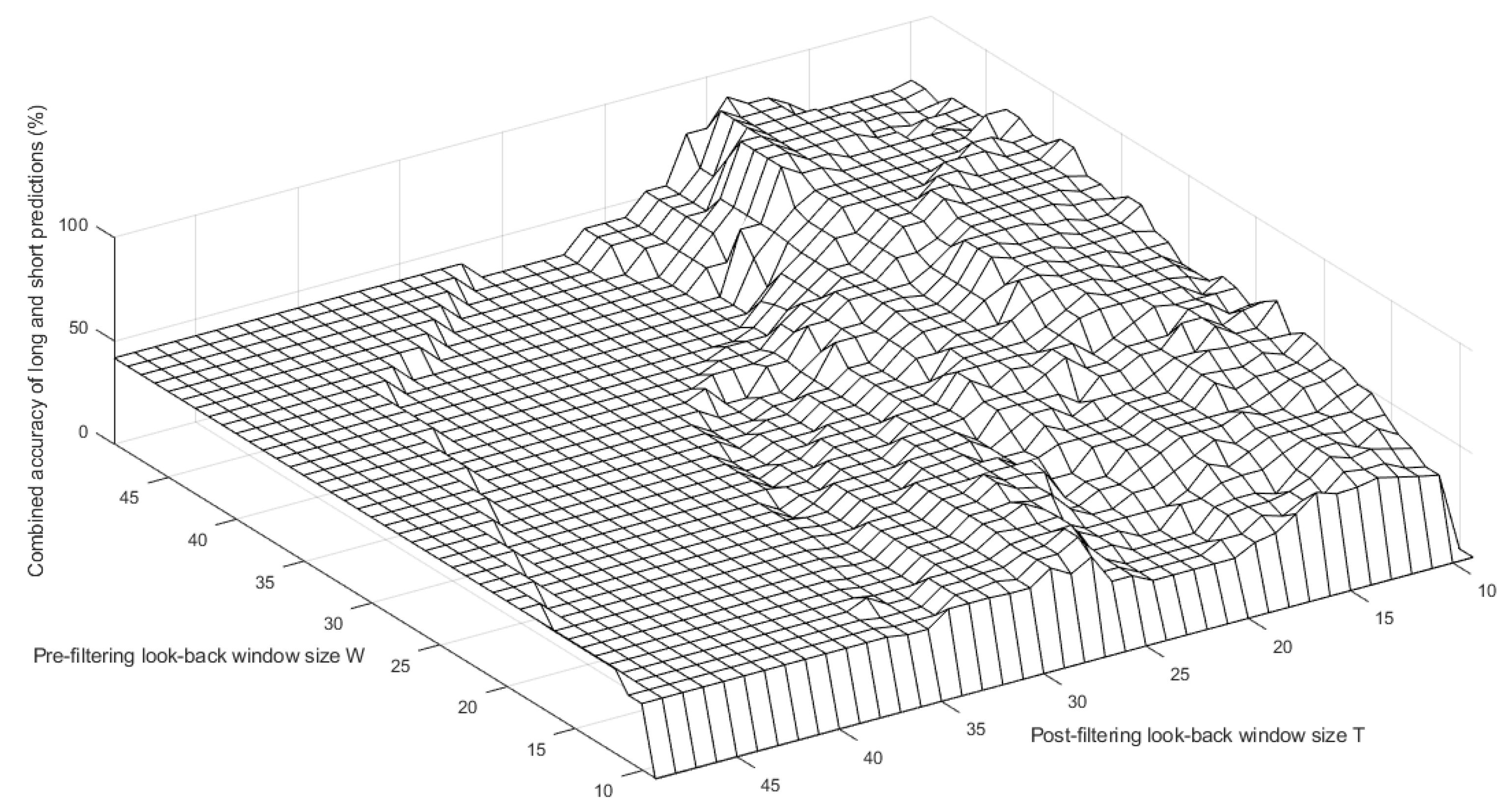
10.1. Pre- and Post-Filtering

As shall be discussed later, the numerical accuracy of results obtained in predicting a trend and its longevity, is critically dependent on the filtering of both the input data and ${\lambda }_{\sigma }$—pre- and post-filtering, respectively.

10.1.1. Pre-Filtering

The positions in time at which the zero crossings are evaluated using Equation (26) depend on the accuracy of the algorithm used to compute ${\lambda }_{\sigma }$ which in turn, depends on the intrinsic noise associated with the time series data. This can yield errors in the positions at which the zero-crossings are computed especially in regard to changes associated with very short time micro-trends.

In the context of longer term macro-trends, such micro-trends may legitimately be interpreted as noise although, in the context of financial times series analysis, for example, the term "noise" must be understood to reflect legitimate price values. To overcome this effect, $u_n$ is filtered using a moving average filter defined by:

$$u\left(t\right):=w\left(t\right)\otimes u\left(t\right)$$

where

$$w\left(t\right)=\left\{\begin{array}{cc}1/W,\hfill & \mid t\mid \le W\hfill \\ 0,\hfill & \mid t\mid >W\hfill \end{array}\right.$$

and W defines the length of the “moving window”. The function given in Appendix A.4 provides a moving average filter for pre-filtering the data $u_n$ using a window of size W.

10.1.2. Post-Filtering

In addition to pre-filtering the time series data, an option for post-filtering the ${\lambda }_{\sigma }$ is required to further control the dynamic behaviour of this index. We therefore again consider a moving average filter given by

$${\lambda }_{\sigma }\left(t\right):=w\left(t\right)\otimes {\lambda }_{\sigma }\left(t\right)$$

where

$$w\left(t\right)=\left\{\begin{array}{cc}1/T,\hfill & \mid t\mid \le T\hfill \\ 0,\hfill & \mid t\mid >T\hfill \end{array}\right.$$

and T defines the length of the “moving window”, $T\ne W$.

10.2. Zero-Crossings Analysis

On the basis of the ideas considered in the previous section, the critical points at which a trend forecasting decision is made are the zero crossing points associated with ${\lambda }_{\sigma }$. By computing ${\lambda }_{\sigma }\left(t\right)$ where t is the position in time of the window, identification of the zero crossings denoted by the function $z_c\left(t\right)$ involves the follow basic procedure:

$$z_c\left(t\right)=\left\{\begin{array}{cc}+1,\hfill & {\lambda }_{\sigma }\left(t\right)<0\&{\lambda }_{\sigma }(t+\epsilon )\ge 0;\hfill \\ -1,\hfill & {\lambda }_{\sigma }\left(t\right)>0\&{\lambda }_{\sigma }(t+\epsilon )\le 0;\hfill \\ 0,\hfill & \mathrm{otherwise}.\hfill \end{array}\right.$$

where $\epsilon$ is a small perturbation in time. This procedure generates a series of Kronecker delta functions whose polarity determines the position(s) in time at which a trend is expected to be positive or negative. Thus the function $z_c\left(t\right)$ identifies the zero crossings associated with the end of an upward trend and the start of a downward trend when $z_c\left(t\right)=-1$ and the end of downward trend and the start of an upward trend when $z_c\left(t\right)=+1$. This is therefore a "critical indicator" in regard to forecasting the trending behaviour of a time series.

10.3. Back-Testing Evaluator

Back-testing algorithms are designed to “gauge” the accuracy of results in terms of trend predictions, for example, and, are usually, but not exclusively, related to testing a strategy for forecasting the behaviour of a financial time series. They are usually designed to assess the overall accuracy of some trading strategy based on historical data when the future outcomes of such a strategy can be evaluated. In this context, the function given in Appendix A.5 evaluates the performance associated with the zero-crossings analysis discussed in the previous section. This evaluation operates on the basis that the price differences should reflect the interval between the start and end points of a predicted trend if the prediction is correct. Thus, in the case when $z_c\left(t\right)>0$ and the trend is positive, the price difference between this point in the time series and the next point in time series when $z_c\left(t\right)<0$ should be positive, thereby representing a net price gain between the two zero crossings. Similarly, when $z_c\left(t\right)<0$ and the trend is negative, the price difference between this point in the time series and the next point in time series when $z_c\left(t\right)>0$ should be negative, thereby representing a net price loss between the two zero crossings. In those cases where this occurs throughout the duration of the time series considered, the predicted entry and exits points are taken to be correct, or else, they are taken to be incorrect. The accuracy associated with this evaluation is computed as a percentage in terms of successful entries and exits, i.e., going “long” (when an investment might be made because the price of a commodity is increasing) and going “short” (when an investment would be held or sold at the start of a downward trend), respectively.

10.4. Example Results

A function called Backtester is provided in Appendix A.6 which gives the user options on the sizes of the look-back window length W and T and the size L of the data stream that is used from the available input data. This data is provided in the form of a column vector via a .txt file. The function normalises this data so that it can be plotted on a scale that is consistent with the scale of ${\lambda }_{\sigma }\left[n\right]$. The function provides a plot which shows the evolution of $u_n$ (normalised), ${\lambda }_{\sigma }\left[n\right]$ and $z_c\left[n\right]$ and then evaluates the results using function evaluator as discussed in the previous section. Note that both the Lyapunov exponent and the volatility are evaluated from the original data (and not the normalised data used for the plot) using a look-back window of T.

Figure 7 shows some example results of running Backtester for the first 1000 elements of the FTSE 100 prices given in Figure 3. The three examples provided are for function Backtester(10,10,1000), Backtester(20,10,1000) and Backtester(30,10,1000) for which the combined entry/exit (long/short) accuracy is 36.55%, 64.58% and 72.73%, respectively. From these results it is clear that the accuracy improves significantly with the extent of the pre-filtering that is applied to the time series before computation of the LVR. This is to be expected as pre-filtering reduces the noise associated with the time series prior to the computation of the LVR.

In order to quantify both the pre- and post-filtering effect on the combined accuracy of the long/short predictions, Figure 8 shows a surface (mesh) plot of the combined accuracy as a function of the pre- and post-filtering look-back window sizes W and T, respectively. The maximum value associated with this ‘$WT$-map’ is 87.5% which occurs at $(W,T)$ coordinates (40, 10). From Figure 8 it can be seen that the highest combined accuracies (>70%) are obtained for approximate values of $W\in [30,50]$ and $T\in [10,20]$. However, it should be noted that $WT$-maps of this kind are data dependent and will vary with the type of financial time series that is processed and on the non-stationary characteristics that occur over the length of the data series that is chosen (i.e., the input parameter L in function Backtester). Hence, $WT$-maps of the type given in Figure 8 provide a “signature” for a financial signal from which optimal values of the pre- and post filtering windows can be established. This optimisation is based on finding the smallest values of W and T that will maintain a combined accuracy compatible with an expected return over a given time scale.

As a comparative example, Figure 9 shows the equivalent $WT$-map for 1000 elements of the Eruo-Dollar (USA) daily (averaged) exchange rates from 29/04/2008 to 27/02/2012 as given in Figure 10. In this case, a maximum value of 83.33% occurs at $WT$ coordinates with minimum values of (38, 12). Although the quantitative details of this $WT$-map are unique to the data used, in qualitative terms, it is similar to the $WT$-map given in Figure 8 revealing that greater accuracy is achieved for large values of W relative to T which is intuitively to be expected. Clearly, for any specific financial date series, a $WT$-map is required to provide an optimal accuracy associated with the trend analysis of that series under the assumption that the stochastic behaviour of the series is stationary, i.e., the financial signal is Ergodic.

11. Price Prediction Using Evolutionary Computing

The trend analysis considered in the previous sections provides evidence of being able to predict a positive or negative trend in a financial signal over a period of time that yields a net positive of negative gradient, respectively, before the trend is reversed. This is based on pre-filtering the financial signal and post-filtering the LVR in which the accuracy achieved is based on the look-back windows of both filters. Such an approach only provides a statement on the expected future trend of a financial signal; it does not provide an estimate of the actual future price.

On the basis of Equation (15) and the random walk hypothesis it represents, it is not possible to determine a future price with 100% accuracy whatever the time scale, given that most financial signals are known to be self-affine stochastic fields which exhibit the same statistical distributions over all time scales. Thus, it is well known and understood (but not always appreciated) that in economics, only an estimate (essentially an informed guess) of a future price is possible. However, in principle, the lower the volatility of the signal, the less likely it is to exhibit large random variation at some future (short) time and hence, the larger the LVR the more likely it is that an estimate of a future price will be a more accurate prediction. In terms of Equation (15), this means that $u(t+\tau )\sim u\left(t\right)$ given that $s\left(t\right)\sim 0$, i.e., ‘tomorrow’s price is likely to be close to today’s price. This provides the basis for using evolutionary computing to estimate short time price values by using the LVR to flag when the approach can be used effectively, i.e., when the LVR reaches a maximum or minimum above or below a certain threshold, respectively—as illustrated in Figure 7 for a threshold of 2, for example.

11.1. Evolutionary Computing

Evolutionary computing (EC) involves “applying the Darwinian principles of natural selection to algorithmic problem solving” [42] and has its origins in the 1960s with the introduction of “evolutionary programming” [43], “genetic algorithms” [44], and “evolutionary strategies” [45]. Following independent developments in the 1990s these areas merged to form the discipline of genetic programming known today as EC in which a correlation exists between natural evolution and evolution by computational problem solving [46].

In the context of a local environment that has a population striving for survival and to reproduce, with natural evolution, the success (fitness) of each individual is dependent on their environment and how well they meet their goals. Similarly, with a trial-and-error mathematical process, a candidate solution is judged in the context of the problem that it is trying to solve and how well the candidate solves the problem which determines whether or not it is kept as a candidate solution. A common theme in EC is the idea of taking a population of individuals “operating” according to environmental pressures causing natural selection and thereby the growth of a fitter population. Many aspects of EC are stochastic and the starting point of candidate solutions can be either deterministic or stochastic. In either case, the aim is to produce a “solution” that minimises some fitness function.

11.2. Eureqa

Eureqa is an EC tool originally developed by the Cornell Creative Machine Laboratory (Cornell University) and commercialised by Nutonian Inc. ( Boston, MA, USA) [47]. The underlying principle is to use genetic programming to generate equations, each of which provides an increasingly better fitness function to model a given dataset. The system iteratively generates a sequence of non-linear functions to describe input (digital) signals which may include stochastic signals [48]. It is a modelling engine predicated on artificial intelligence using evolutionary searches to determine an equation that represents a set of data [49]. The system automatically discovers formulae through evolutionary algorithms requiring no human intervention starting by randomly creating equations via sequences of mathematical building blocks based on a combination of common functions. The content of these formulae is ordered only by a basic syntax (e.g., two addition signs cannot appear one after the other). Beyond this basic syntax, the sequences generated by the program are entirely random.

11.3. Application to Financial Forecasting

With a little data “Eureqa generates fundamental laws of nature” [50]. However, there have been few applications of EC to financial forecasting. This is partly due to the significance of Equation (15) and the basic random walk hypothesis which financial signals adhere to, albeit as self-affine stochastic fields. Thus although EC can be used to generate a non-linear equation for some short time financial signal, no fundamental significance in terms of a “law of nature” can be inferred by such an equation due to the random walk nature of the data that is used. To date, the only “law of nature” that can be used to describe financial signals is that they are statistically self-affine fields to which the fractal market hypothesis is thereby applicable. Nevertheless, EC can be used to provide short time predictions including the performance of equity markets [51] and energy commodities [52], for example. This is done by using EC to generate representative equations for existing prices over a look-back window and can, in principle, be applied successive for a moving (look-back) window especially for time periods where the volatility of the time series is low and future prices can be expected to be random but locally similar to past prices.

11.4. An Example Result

With reference to Figure 7, we consider the daily prices for array values between 870 and 900 (inclusively) which correspond to days 24/08/2009 to 08/09/2009 when the LVR is ∼3 and relatively flat. With these 30 price values, Eureqa provides the following formula:

$$\begin{array}{cc}\hfill f\left(t\right)& =5025.73417939762+8.96527863946579t^2+1.52597679067939\times {10}^{-6}{t}^6\hfill \\ \hfill & +cos\left(8.96527863946579t\right)-76.8453768284695t-0.253321938783733t^3\hfill \\ \hfill & -48.5578781261177sin(0.96446841878421+7.16244232473996t)\hfill \end{array}$$

(27)

obtained after 51,056 generations giving a correlation coefficient of 0.98362871, an $R^2$ (coefficient of determination) goodness of fit of 0.96684623, a mean absolute error of 16.623419 and a complexity of 51.

Figure 11 shows a comparison of the true price values with the estimates obtained using a discretised version of Equation (27) given by

$$\begin{array}{cc}\hfill f_n& =5025.73417939762+8.96527863946579t_n^2+1.52597679067939\times {10}^{-6}{t}_n^6\hfill \\ \hfill & +cos\left(8.96527863946579t_n\right)-76.8453768284695t_n-0.253321938783733t_n^3\hfill \\ \hfill & -48.5578781261177sin(0.96446841878421+7.16244232473996t_n),n=1,2,\dots ,N,t_n=n\hfill \end{array}$$

(28)

for $N=30$, and, additionally, for $n=31,32$ and 33 thereby providing future price prediction for three days ahead.

A comparison of the numerical values for these price predictions is given in

Table 2. Table comparing the actual and predicted prices for three days of the FTSE100 using Equation (28).

Day	09/09/2009	10/09/2009	11/09/2009
$t_n$	31	32	33
Predicted price value $f_n$	5022.9	5066.6	5087.4
Actual price value $u_n$	5138.0	5108.9	5154.6

.

11.5. Discussion

With reference to Figure 11, the local trend in prices before and inclusive of element 30 (i.e., elements 26–30) is downward and so based on the principle of Equation (15) for $s\left(t\right)\sim 0$ and application of exponential smoothing for time series forecasting [53], for example, continuation of this trend will lead to inaccurate predictions that are inconsistent with the local increase in prices for elements 31, 32 and 33—the circled dots in Figure 11. However, the equivalent future predictions given by Equation (28) are consistent with the actual values which represent a short time up-ward trend as shown in Table 2. The predictive ability of EC can only be considered for very short future time increments (a look-forward prediction window) but this example result does provide evidence for the success of using EC exercised on a moving look-back window basis.

A quantitative study on the accuracy of this approach in terms of the look-back window and the look-forward (prediction) window relative to the local LVR lies beyond the scope of this work. However, it is to be expected that the success of this approach will be predicated on the size of the amplitude of $\mid {\lambda }_{\sigma }\mid$ when the volatility is low. Hence, based on the results given in Figure 7, an EC moving window approach may be used when $\mid {\lambda }_{\sigma }\mid \ge 2$ where ${\lambda }_{\sigma }$ is given by Equation (26). In this context, the LVR not only provides a method of predicting trends (subject to appropriate pre- and post-filtering) based on its change in polarity but also flags when to apply EC to generate future price estimates.

12. Derivations of the Diffusion Equation from the Evolution Equation

So far in this paper, we have developed a predictive indicator that is based on combining the Lyapunov exponent and the volatility into a ratio (the LVR), both parameters having been derived from E${}^3$ and computed on a moving window basis. We have then used the amplitude of this ratio to gauge the likelihood of using EC to successfully predict short term future price values. We have not yet studied the effect of applying specific models for the PDF associated with E${}^3$ which is the subject of later sections. In particular, we show how the classical diffusion equation is a result of considering a Gaussian PDF in E${}^3$ and the non-classical fractional diffusion equation is the result of considering a non-Gaussian PDF, in particular, a Lévy distribution and undertaken using the associated characteristic functions.

In this section we consider three approaches to deriving the classical diffusion equation in order to show the connectivity between this equation and E${}^3$ in terms of applying different conditions and approximations. We start with Einstein’s original approach which is independent of the specific PDF but on the condition that the PDF is symmetric.

12.1. Einstein’s Derivation for $\mathbf{r}\in {\mathbb{R}}^1$

In his 1905 paper [1], Einstein considered the one-dimensional case, when $\mathbf{r}\in {\mathbb{R}}^1$, and where the PDF is taken to be symmetric so that $p\left(x\right)=p(-x)$. In this case, Equation (10) can be written as

$$u(x,t+\tau )=\underset{-\infty }{\overset{\infty }{\int }}p(x-\lambda )u(\lambda ,t)d\lambda =\underset{-\infty }{\overset{\infty }{\int }}p(x+\lambda )u(\lambda ,t)d\lambda =\underset{-\infty }{\overset{\infty }{\int }}p\left(\lambda \right)u(x+\lambda ,t)d\lambda$$

Taylor expanding $u(x,t)$ to first order in time, and, to second order in space, we then obtain

$$u(x,t)+\tau \frac{\partial }{\partial t}u(x,t)=\underset{-\infty }{\overset{\infty }{\int }}d\lambda p\left(\lambda \right)\left[u(x,t)+\lambda \frac{\partial }{\partial x}u(x,t)+\frac{{\lambda }^2}{2}\frac{{\partial }^2}{\partial x^2}u(x,t)\right]$$

$$=u(x,t)\underset{-\infty }{\overset{\infty }{\int }}p\left(\lambda \right)d\lambda +\frac{\partial }{\partial x}u(x,t)\underset{-\infty }{\overset{\infty }{\int }}\lambda p\left(\lambda \right)d\lambda +\frac{{\partial }^2}{\partial x^2}u(x,t)\underset{-\infty }{\overset{\infty }{\int }}\frac{{\lambda }^2}{2}p\left(\lambda \right)d\lambda$$

$$=u(x,t)+\frac{{\partial }^2}{\partial x^2}u(x,t)\underset{-\infty }{\overset{\infty }{\int }}\frac{{\lambda }^2}{2}p\left(\lambda \right)d\lambda$$

since

$$\underset{-\infty }{\overset{\infty }{\int }}p\left(\lambda \right)d\lambda =1\mathrm{and}\underset{-\infty }{\overset{\infty }{\int }}\lambda p\left(\lambda \right)d\lambda =0.$$

We can thus write the equation

$$\frac{\partial }{\partial t}u(x,t)=D\frac{{\partial }^2}{\partial x^2}u(x,t)$$

(29)

where

$$D=\underset{-\infty }{\overset{\infty }{\int }}\frac{{\lambda }^2}{2\tau }p\left(\lambda \right)d\lambda .$$

(30)

which is the one-dimensional diffusion equation for diffusivity D with dimensions of Length${}^2$/Time. This derivation of the diffusion equation relies on the conditions $\tau <<1$ and ${\lambda }^2<<1$ which are required in order to truncate the Taylor series expansion of $u(x,t+\tau )$ in time and $u(x+\lambda ,t)$ in space. However, this derivation of the diffusion equation is independent of the PDF (subject to the condition that the PDF is symmetric) which determines the diffusivity D through Equation (30).

12.2. Einstein’s Derivation for $\mathbf{r}\in {\mathbb{R}}^3$

A similar approach can be used to deriving of the diffusion equation for $\mathbf{r}\in {\mathbb{R}}^3$ as shall now be demonstrated. In this case

$$u(\mathbf{r},t+\tau )=p\left(r\right)\otimes u(\mathbf{r},t),p\left(r\right)=p(-r)$$

can be written out in the form

$$u(\mathbf{r},t+\tau )=\underset{-\infty }{\overset{\infty }{\int }}u(\mathbf{r}+\lambda ,t)p\left(\lambda \right)d\lambda$$

where $\lambda$ is a scalar with dimensions of length and components ${\lambda }_x,{\lambda }_y$ and ${\lambda }_z$. Expanding $u(\mathbf{r}+\lambda ,t)$ in terms of a three-dimensional Taylor series,

$$u(\mathbf{r}+\lambda ,t)=u(\mathbf{r},t)+{\lambda }_x\frac{\partial u(\mathbf{r},t)}{\partial x}+{\lambda }_y\frac{\partial u(\mathbf{r},t)}{\partial y}+{\lambda }_z\frac{\partial u(\mathbf{r},t)}{\partial z}+\frac{{\lambda }_x^2}{2!}\frac{{\partial }^{2}u(\mathbf{r},t)}{\partial x^2}+\frac{{\lambda }_y^2}{2!}\frac{{\partial }^{2}u(\mathbf{r},t)}{\partial y^2}+\frac{{\lambda }_z^2}{2!}\frac{{\partial }^{2}u(\mathbf{r},t)}{\partial z^2}$$

$$+{\lambda }_x{\lambda }_y\frac{{\partial }^{2}u(\mathbf{r},t)}{\partial x\partial y}+{\lambda }_x{\lambda }_z\frac{{\partial }^{2}u(\mathbf{r},t)}{\partial x\partial z}+{\lambda }_y{\lambda }_z\frac{{\partial }^{2}u(\mathbf{r},t)}{\partial y\partial z}+\dots$$

so that, for $\tau <<1$,

$$u(\mathbf{r},t)+\tau \frac{\partial u(\mathbf{r},t)}{\partial t}=\underset{-\infty }{\overset{\infty }{\int }}u(\mathbf{r},t)p\left(\lambda \right)d\lambda +\underset{-\infty }{\overset{\infty }{\int }}\left({\lambda }_x\frac{\partial u(\mathbf{r},t)}{\partial x}+{\lambda }_y\frac{\partial u(\mathbf{r},t)}{\partial y}+{\lambda }_z\frac{\partial u(\mathbf{r},t)}{\partial z}\right)p\left(\lambda \right)d\lambda$$

$$+\underset{-\infty }{\overset{\infty }{\int }}\left(\frac{{\lambda }_x^2}{2!}\frac{{\partial }^{2}u(\mathbf{r},t)}{\partial x^2}+\frac{{\lambda }_y^2}{2!}\frac{{\partial }^{2}u(\mathbf{r},t)}{\partial y^2}+\frac{{\lambda }_z^2}{2!}\frac{{\partial }^{2}u(\mathbf{r},t)}{\partial z^2}\right)p\left(\lambda \right)d\lambda$$

$$+\underset{-\infty }{\overset{\infty }{\int }}\left({\lambda }_x{\lambda }_y\frac{{\partial }^{2}u(\mathbf{r},t)}{\partial x\partial y}+{\lambda }_x{\lambda }_z\frac{{\partial }^{2}u(\mathbf{r},t)}{\partial x\partial z}+{\lambda }_y{\lambda }_z\frac{{\partial }^{2}u(\mathbf{r},t)}{\partial y\partial z}\right)p\left(\lambda \right)d\lambda$$

We then obtain

$$\begin{array}{cc}\hfill \tau \frac{\partial }{\partial t}u(\mathbf{r},t)=& \underset{-\infty }{\overset{\infty }{\int }}\frac{{\lambda }_x^2}{2}\frac{{\partial }^{2}u(\mathbf{r},t)}{\partial x^2}p\left(\lambda \right)d\lambda +\underset{-\infty }{\overset{\infty }{\int }}\frac{{\lambda }_x{\lambda }_y}{2}\frac{{\partial }^{2}u(\mathbf{r},t)}{\partial x\partial y}p\left(\lambda \right)d\lambda +\underset{-\infty }{\overset{\infty }{\int }}\frac{{\lambda }_x{\lambda }_z}{2}\frac{{\partial }^{2}u(\mathbf{r},t)}{\partial x\partial z}p\left(\lambda \right)d\lambda \hfill \\ \hfill & +\underset{-\infty }{\overset{\infty }{\int }}\frac{{\lambda }_y{\lambda }_x}{2}\frac{{\partial }^{2}u(\mathbf{r},t)}{\partial y\partial x}p\left(\lambda \right)d\lambda +\underset{-\infty }{\overset{\infty }{\int }}\frac{{\lambda }_y^2}{2}\frac{{\partial }^{2}u(\mathbf{r},t)}{\partial y^2}p\left(\lambda \right)d\lambda +\underset{-\infty }{\overset{\infty }{\int }}\frac{{\lambda }_y{\lambda }_z}{2}\frac{{\partial }^{2}u(\mathbf{r},t)}{\partial y\partial z}p\left(\lambda \right)d\lambda \hfill \\ \hfill & +\underset{-\infty }{\overset{\infty }{\int }}\frac{{\lambda }_z{\lambda }_x}{2}\frac{{\partial }^{2}u}{\partial z\partial x}p\left(\lambda \right)d\lambda +\underset{-\infty }{\overset{\infty }{\int }}\frac{{\lambda }_z{\lambda }_y}{2}\frac{{\partial }^{2}u(\mathbf{r},t)}{\partial z\partial y}p\left(\lambda \right)d\lambda +\underset{-\infty }{\overset{\infty }{\int }}\frac{{\lambda }_z^2}{2}\frac{{\partial }^{2}u(\mathbf{r},t)}{\partial z^2}p\left(\lambda \right)d\lambda \hfill \\ \hfill & +\underset{-\infty }{\overset{\infty }{\int }}{\lambda }_x\frac{\partial u(\mathbf{r},t)}{\partial x}p\left(\lambda \right)d\lambda +\underset{-\infty }{\overset{\infty }{\int }}{\lambda }_y\frac{\partial u(\mathbf{r},t)}{\partial y}p\left(\lambda \right)d\lambda +\underset{-\infty }{\overset{\infty }{\int }}{\lambda }_z\frac{\partial u(\mathbf{r},t)}{\partial z}p\left(\lambda \right)d\lambda \hfill \end{array}$$

which can be written as

$$\frac{\partial }{\partial t}u(\mathbf{r},t)=\nabla ·\mathbf{D}\nabla u(\mathbf{r},t)+\mathbf{V}·\nabla u(\mathbf{r},t)$$

where $\mathbf{D}$ is the diffusion tensor given by

$$\mathbf{D}=\left(\begin{array}{ccc}{D}_{xx}& D_{xy}& D_{xz}\\ D_{yx}& D_{yy}& D_{yz}\\ D_{zx}& D_{zy}& D_{zz}\end{array}\right),D_{ij}=\underset{-\infty }{\overset{\infty }{\int }}\frac{{\lambda }_i{\lambda }_j}{2\tau }p\left(\lambda \right)d\lambda$$

and $\mathbf{V}$ is a flow vector which describes any drift velocity that the particle ensemble may have and is given by

$$\mathbf{V}=\left(\begin{array}{c}{V}_x\\ V_y\\ V_z\end{array}\right),V_i=\underset{-\infty }{\overset{\infty }{\int }}\frac{{\lambda }_i}{\tau }p\left(\lambda \right)d\lambda .$$

Note that as ${\lambda }_i{\lambda }_j={\lambda }_j{\lambda }_i$, the diffusion tensor is diagonally symmetric (i.e., $D_{ij}=D_{ji}$). For isotropic diffusion when $\langle {\lambda }_i{\lambda }_j\rangle =0$ for $i\ne j$ and $\langle {\lambda }_i{\lambda }_j\rangle =\langle {\lambda }^2\rangle$ for $i=j$ and with a zero drift velocity when $\mathbf{V}=\mathbf{0}$,

$$\frac{\partial }{\partial t}u(\mathbf{r},t)=\nabla ·\left(\begin{array}{ccc}D& 0& 0\\ 0& D& 0\\ 0& 0& D\end{array}\right)\nabla u(\mathbf{r},t)=D{\nabla }^{2}u(\mathbf{r},t),D=\underset{-\infty }{\overset{\infty }{\int }}\frac{{\lambda }^2}{2\tau }p\left(\lambda \right)d\lambda$$

12.3. PDF Dependent Derivation of the Diffusion Equation

Consider the case when, for  $\mathbf{r}\in {\mathbb{R}}^1$, $p\left(x\right)$ is a zero-mean normal (Gaussian) distribution with Standard Deviation $\sigma$ and Variance ${\sigma }^2$, i.e.,

$$p\left(x\right)=\frac{1}{\sqrt{2\pi {\sigma }^2}}exp\left(-\frac{x^2}{2{\sigma }^2}\right),$$

Taylor expansion to first order of Equation (10) followed by application of the convolution theorem yields the Fourier space equation

$$U(k,t)+\tau \frac{\partial }{\partial t}U(k,t)=P\left(k\right)U(k,t)$$

(31)

where

$$U(k,t)=\underset{-\infty }{\overset{\infty }{\int }}u(x,t)exp(-ikx)dx$$

and

$$P\left(k\right)=\underset{-\infty }{\overset{\infty }{\int }}p\left(x\right)exp(-ikx)dx=exp\left(-\frac{{\sigma }^2{k}^2}{2}\right),$$

$P\left(k\right)$ being the Characteristic Function.

Suppose we now consider the case when the variance is small, i.e., ${\sigma }^2<<1$. Then

$$P\left(k\right)=1-\frac{{\sigma }^2{k}^2}{2}+\frac{1}{2!}{\left(\frac{{\sigma }^2{k}^2}{2}\right)}^2+\dots \sim 1-\frac{{\sigma }^2{k}^2}{2},{\left(\sigma k\right)}^2<<1$$

and Equation (31) can be written as

$$\frac{\partial }{\partial t}U(k,t)=-U(k,t)\frac{{\sigma }^2{k}^2}{2\tau }$$

through which we again obtain the diffusion equation

$$\frac{\partial }{\partial t}u(x,t)=D\frac{{\partial }^2}{\partial x^2}u(x,t)\mathrm{where}D=\frac{{\sigma }^2}{2\tau }$$

given that

$$-k^{2}U(k,t)\leftrightarrow \frac{{\partial }^2}{\partial x^2}u(x,t).$$

In this case, the “key” to the derivation of the diffusion equation is the assumption that the variance of a normal distribution is small and that $\tau <<1$. We note that an identical analysis in the two- and three-dimensional domains yields the the two- and three-dimensional diffusion equation

$$\frac{\partial }{\partial t}u(\mathbf{r},t)=D{\nabla }^{2}u(\mathbf{r},t),\mathbf{r}\in {\mathbb{R}}^n,n=2,3$$

12.4. Generalisation

We can generalise this approach further by writing the evolution equation in Fourier space using the convolution theorem and in expanded form as

$$U(\mathbf{k},t)+\tau \frac{\partial }{\partial t}U(\mathbf{k},t)+\frac{{\tau }^2}{2!}\frac{{\partial }^2}{\partial t^2}U(\mathbf{k},t)+\dots =U(\mathbf{k},t)-\tau D{k}^{2}U(\mathbf{k},t)+\frac{{\tau }^2}{2!}{D}^2{k}^{4}U(\mathbf{k},t)-\dots$$

so that upon inverse Fourier transformation we have, for $\mathbf{r}\in {\mathbb{R}}^n,n=1,2,3$

$$\tau \frac{\partial }{\partial t}u(\mathbf{r},t)+\frac{{\tau }^2}{2!}\frac{{\partial }^2}{\partial t^2}u(\mathbf{r},t)+\dots =\tau D{\nabla }^{2}u(\mathbf{r},t)-\frac{{\tau }^2}{2!}{D}^2{\nabla }^4+\dots$$

Equating terms with the same coefficients in regard to powers of $\tau$, we have (for any positive integer m)

$$\frac{\partial }{\partial t}u(\mathbf{r},t)=D{\nabla }^{2}u(\mathbf{r},t),\frac{{\partial }^2}{\partial t^2}u(\mathbf{r},t)=D^2{\nabla }^{4}u(\mathbf{r},t),\dots ,\frac{{\partial }^m}{\partial t^m}u(\mathbf{r},t)=D^m{\nabla }^{m+2}u(\mathbf{r},t)$$

Since all such equations can be constructed from the diffusion equation, i.e.,

$$\frac{{\partial }^2}{\partial t^2}u(\mathbf{r},t)=D{\nabla }^2\frac{\partial }{\partial t}u(\mathbf{r},t)=D{\nabla }^2\left[D{\nabla }^{2}u(\mathbf{r},t)\right],\dots$$

this analysis confirms that the diffusion equation is E${}^3$ for the case when the PDF is a Gaussian distribution.

12.5. Green’s Function Solution

For the initial condition $u_0\left(\mathbf{r}\right)\equiv u(\mathbf{r},t=0),\mathbf{r}\in {\mathbb{R}}^n,n=1,2,3$ and in the infinite domain, the Green’s function solution to the homogeneous diffusion equation is [54]

$$u(\mathbf{r},t)=G(\mathbf{r},t)\otimes u_0\left(\mathbf{r}\right)$$

where $G(\mathbf{r},t)$ is the Green’s function given by

$$G(\mathbf{r},t)={\left(\frac{1}{4\pi Dt}\right)}^{\frac{n}{2}}exp\left(-\frac{r^2}{4Dt}\right),t>0;n=1,2,3.$$

12.6. The Black–Scholes Model

There is a synergy associated with the diffusion equation and the Black–Scholes model for a call premium which is compounded in the partial differential equation [55]

$$\frac{\partial }{\partial t}c(x,t)+\frac{1}{2}{\sigma }^2{s}^2\frac{{\partial }^2}{\partial s^2}c(x,t)+rs\frac{\partial }{\partial s}c(x,t)-rc(x,t)=0$$

where $c(x,t)$ is the call premium, s is the stock price, $\sigma$ is the volatility and r is the risk. Subject to specific initial and boundary conditions, this equation can be transformed into the classical diffusion equation through application of a change of variables when it can be written in the form

$$\frac{\partial }{\partial \tau }u(x,\tau )+\frac{1}{2}{\sigma }^2\frac{{\partial }^2}{\partial x^2}u(x,t)$$

which has the same Green’s function solution as given in the previous section, for $n=1$ and initial condition $u(x,t=0)$. Thus, just as the classical diffusion equation is a manifestation of the PDF associated with E${}^3$ being normal, so the Black-Scholes model may be taken to be predicated on Gaussian processes.

13. The Fractional Diffusion Equation

The fractional diffusion equation (FDE) can be derived by generalising the Gaussian characteristic function $P\left(k\right)=exp\left(-{\sigma }^2{k}^2/2\right)$ to the form

$$P\left(k\right)=exp\left(-c\mid k{\mid }^{\gamma }\right)$$

where $\gamma \in [0,2]$ is the Lévy index and c is a constant with dimensions of Length${}^{\gamma }$ as previously discussed in Section 7.2.

Using the Reisz definition of the fractional Laplacian operator ${\nabla }^{\gamma },\mathbf{r}\in {\mathbb{R}}^n$, namely,

$${\nabla }^{\gamma }\leftrightarrow -\mid \mathbf{k}{\mid }^{\gamma }$$

with $D_{\gamma }=c/\tau$, repetition of the analysis given in Section 12.4 yields the homogeneous FDE

$$\frac{\partial }{\partial t}u(\mathbf{r},t)=D_{\gamma }{\nabla }^{\gamma }u(\mathbf{r},t)$$

where $D_{\gamma }$ is the fractional diffusivity with dimensions of Length${}^{\gamma }$/Time, and, for $\mathbf{r}\in {\mathbb{R}}^3$ with Cartesian coordinates $(x,y,z)$,

$${\nabla }^{\gamma }\equiv \frac{{\partial }^{\gamma }}{\partial \mid x{\mid }^{\gamma }}+\frac{{\partial }^{\gamma }}{\partial \mid y{\mid }^{\gamma }}+\frac{{\partial }^{\gamma }}{\partial \mid z{\mid }^{\gamma }}$$

Thus, we obtain a fundamental connectivity between between Einstein’s evolution equation and fractional calculus, i.e., application of the Lévy distribution in Equation (10) yields the FDE.

13.1. Continuity Equation

For the case when $\gamma =1$, we can use the FDE to construct the transport equation

$$\frac{\partial }{\partial t}u(\mathbf{r},t)+D_1\widehat{\mathbf{n}}·\nabla u(\mathbf{r},t)=0$$

where $\widehat{\mathbf{n}}$ is the unit vector. This is a continuity equation, and, in the context of the evolution equation, illustrates the connectivity between the concept of flux (the flow of an ensemble of particles) and the Cauchy distribution (as discussed in Section 7.2).

13.2. Time-Independent Analysis

If we consider Equation (11), then for the time dependent case the FDE becomes

$${\nabla }^{\gamma }u\left(\mathbf{r}\right)=s\left(\mathbf{r}\right),r\in {\mathbb{R}}^n$$

where $u\left(\mathbf{r}\right)$ is a stochastic function. Since ${\nabla }^{\gamma }u\left(\mathbf{r}\right)\leftrightarrow -\mid \mathbf{k}{\mid }^{\gamma }$ we can construct the solution

$$u\left(\mathbf{r}\right)={\mathcal{F}}_n^{-1}\left[\frac{S\left(\mathbf{k}\right)}{\mid \mathbf{k}{\mid }^{\gamma }}\right],S\left(\mathbf{k}\right)\leftrightarrow s\left(\mathbf{r}\right)$$

Using Equation (4) and the convolution theorem, we can then write $u\left(\mathbf{r}\right)$ as

$$u\left(\mathbf{r}\right)=\frac{c_{n,\gamma }}{{\left(2\pi \right)}^n}\frac{1}{\mid \mathbf{r}{\mid }^{n-\gamma }}\otimes s\left(\mathbf{r}\right),0<\mathrm{Re}\left[\gamma \right]<n;c_{n,\gamma }={\pi }^{\frac{n}{2}}{2}^{n-\gamma }\frac{\Gamma \left(\frac{n-\gamma }{2}\right)}{\Gamma \left(\frac{\gamma }{2}\right)}.$$

This solution for $u\left(\mathbf{r}\right)$ defines the Riesz potential and has a fundamental scaling property obtained by considering the convolution of the source function for a scaling factor $\lambda$ when it is simple to show that

$$\frac{c_{n,\gamma }}{{\left(2\pi \right)}^n}\frac{1}{\mid \mathbf{r}{\mid }^{n-\gamma }}\otimes s\left(\lambda \mathbf{r}\right)=\frac{1}{{\lambda }^{\gamma }}u\left(\lambda \mathbf{r}\right)$$

and hence $u\left(\mathbf{r}\right)$ is a scale-invariant stochastic function defined by the relationship

$$\mathrm{Pr}\left[u\left(\lambda \mathbf{r}\right)\right]={\lambda }^{\gamma }\mathrm{Pr}\left[u\left(\mathbf{r}\right)\right].$$

(32)

Thus, for a stochastic source, the Riesz potential $u\left(\mathbf{r}\right)$ is a random scaling self-affine field—a random scaling fractal. In this context, Appendix B develops the relationship between the topological dimension n, the fractal dimension D and the Lévy index $\gamma$ which is given by

$$D=\frac{3n+2-2\gamma }{2}.$$

(33)

Thus, for example, a Mandelbrot surface, which has a fractal dimension $D=4-\gamma \in [2,3]$, can be defined in terms of the solution to the two-dimensional fractional Poisson equation (FPE)

$${\nabla }^{\gamma }u\left(\mathbf{r}\right)=s\left(\mathbf{r}\right),r\in {\mathbb{R}}^2,\gamma \in [2,1]$$

and if $s\left(\mathbf{r}\right)$ has a white spectrum, i.e., a spectrum whose power spectral density function (PSDF) is a constant, then the PSDF of $u\left(\mathbf{r}\right)$ is determined by $1/\mid \mathbf{k}{\mid }^{4-\gamma }$.

We note that by Taylor expanding Equation (11) for the time-independent case, then in Fourier space, we obtain $U\left(\mathbf{k}\right)=P\left(\mathbf{k}\right)U\left(\mathbf{k}\right)+S\left(\mathbf{k}\right)$ and with $P\left(\mathbf{k}\right)=exp(-c\mid \mathbf{k}{\mid }^{\gamma })$ it can be shown that  [37]

$$u\left(\mathbf{r}\right)={\mathcal{F}}_n^{-1}\left[\frac{S\left(\mathbf{k}\right)}{1-exp(-c\mid \mathbf{k}{\mid }^{\gamma })}\right]\sim \frac{1}{r^{n+\gamma }}\otimes s\left(\mathbf{r}\right),r\to \infty ;r\in {\mathbb{R}}^n$$

This asymptotic result yields a similar inverse power law but with the scaling law,

$$\mathrm{Pr}\left[u\left(\mathbf{r}\right)\right]={\lambda }^{\gamma }\mathrm{Pr}\left[u\left(\lambda \mathbf{r}\right)\right],$$

a result that is a characteristic of scale-invariant field theory when the field equations are scale invariant so that for any solution $\varphi \left(\mathbf{r}\right)$, say, of the field equations, there exist other solutions of the form ${\lambda }^{\Delta }\varphi \left(\mathbf{r}\right)$ for an exponent $\Delta$ (not necessarily related to $\gamma$).

13.3. Time-Dependent Analysis

We study the FDE with $\mathbf{r}\in {\mathbb{R}}^1$ for a stochastic source, namely,

$$\left(D_{\gamma }\frac{{\partial }^{\gamma }}{\partial \mid x{\mid }^{\gamma }}-\frac{\partial }{\partial t}\right)u(x,t)=-s(x,t)$$

(34)

and consider the generic Green’s function solution

$$u(x,t)=g(x,t)\otimes s(x,t)$$

where the convolution operation is taken to apply to both x and t. We are then required to compute the Green’s function in this case.

13.4. Green’s Function for the Fractional Diffusion Equation

We consider an evaluation of the Green’s function for the fractional diffusion equation which is defined as the solution to

$$\left(D_{\gamma }\frac{{\partial }^{\gamma }}{\partial \mid x{\mid }^{\gamma }}-\frac{\partial }{\partial t}\right)g(\mid x\mid ,t)=-\delta (\mid x\mid )\delta \left(t\right),t\ge 0.$$

(35)

Writing the Green’s function in terms of the Fourier transformation

$$g(\mid x\mid ,t)=\frac{1}{{\left(2\pi \right)}^2}\underset{-\infty }{\overset{\infty }{\int }}G(k,\omega )exp(ik\mid x\mid )exp\left(i\omega t\right)dkd\omega$$

noting that

$$\delta (\mid x\mid )=\frac{1}{2\pi }\underset{-\infty }{\overset{\infty }{\int }}exp(ik\mid x\mid )dk,\mathrm{and}\delta \left(t\right)=\frac{1}{2\pi }\underset{-\infty }{\overset{\infty }{\int }}exp\left(i\omega t\right)d\omega$$

and using the Reisz definition of a fractional derivative, Equation (35) becomes

$$[-D_{\gamma }\mid k{\mid }^{\gamma }-\left(i\omega \right)]G(k,\omega )=-1$$

which can be written in the factored form

$$\left[(\mid k{\mid }^{\gamma /2}+{(-i\omega /D_{\gamma })}^{1/2})(\mid k{\mid }^{\gamma /2}-{(-i\omega /D_{\gamma })}^{1/2})\right]G(k,\omega )=\frac{1}{D_{\gamma }}.$$

(36)

It is well known that for the equation

$$\left(D_{\gamma }\frac{{\partial }^2}{\partial x^2}-\frac{{\partial }^2}{\partial t^2}\right)g(\mid x\mid ,t)=-\delta (\mid x\mid )\delta \left(t\right),$$

$$(k^2-{\omega }^2/D_{\gamma })G(k,\omega )=\frac{1}{D_{\gamma }}\mathrm{or}\left[(k+\omega /\sqrt{D_{\gamma }})(k-\omega /\sqrt{D_{\gamma }})\right]G(k,\omega )=\frac{1}{D_{\gamma }}$$

and the outgoing Green’s function is given by

$$\tilde{g}(x\mid x_0,\omega )=\frac{i}{2\omega \sqrt{D_{\gamma }}}exp[i(\omega /\sqrt{D_{\gamma }})\mid x\mid ].$$

(37)

Generalising this result for Equation (36), we therefore consider the expression

$$\tilde{g}(\mid x\mid ,\omega )=\frac{i}{2D_{\gamma }{(-i\omega /D_{\gamma })}^{1/\gamma }}exp[i{(-i\omega /D_{\gamma })}^{1/\gamma }\mid x\mid ],$$

(38)

given that when $\gamma =2$ and $-i\omega /D_{\gamma }:={\omega }^2/D_{\gamma }$, Equation (37) is recovered.

To find the time evolution of the Green’s function, we are required to take the inverse Fourier transform of $\tilde{g}(\mid x\mid ,\omega )$, and evaluate the integral

$$g(\mid x\mid ,t)=\frac{1}{2\pi }\underset{-\infty }{\overset{\infty }{\int }}\frac{i}{2D_{\gamma }{(-i\omega /D_{\gamma })}^{1/\gamma }}exp[i{(-i\omega /D_{\gamma })}^{1/\gamma }\mid x\mid ]exp\left(i\omega t\right)d\omega .$$

(39)

This can be achieved by writing the exponential function $exp[i{(-i\omega /D_{\gamma })}^{1/\gamma }\mid x\mid ]$ as a series which yields the series solution

$$\begin{array}{cc}\hfill g(\mid x\mid ,t)& =\frac{i}{2D_{\gamma }}{\mathcal{F}}_n^{-1}\left[\frac{1}{{(-i\omega /D_{\gamma })}^{1/\gamma }}+i\mid x\mid +\sum _{n=2}^{\infty }\frac{i^n}{n!}{(-i\omega /D_{\gamma })}^{(n-1)/\gamma }\mid x{\mid }^n\right]\hfill \\ \hfill & =\frac{i}{2D_{\gamma }}{\mathcal{F}}_n^{-1}\left[\frac{D_{\gamma }^{1/\gamma }}{{(-1)}^{1/\gamma }{\left(i\omega \right)}^{1/\gamma }}+i\mid x\mid +\sum _{n=2}^{\infty }\frac{i^n}{n!}{\left(\frac{-1}{D_{\gamma }}\right)}^{(n-1)/\gamma }{\left(i\omega \right)}^{(n-1)/\gamma }\mid x{\mid }^n\right]\hfill \\ \hfill & =\frac{i}{2D_{\gamma }}\left[\frac{D_{\gamma }^{1/\gamma }}{{(-1)}^{1/\gamma }\Gamma (1/\gamma )}\frac{H\left(t\right)}{t^{1-1/\gamma }}+i\mid x\mid \delta \left(t\right)+\sum _{n=2}^{\infty }\frac{i^n}{n!}{\left(\frac{-1}{D_{\gamma }}\right)}^{(n-1)/\gamma }\mid x{\mid }^n{\delta }^{\left[\right(n-1)/\gamma ]}\left(t\right)\right]\hfill \end{array}$$

(40)

where

$$H\left(t\right)=\underset{-\infty }{\overset{t}{\int }}\delta \left(s\right)ds$$

is the Heaviside step function. This result comes from noting that for $0<\alpha <1$

$$\frac{1}{\Gamma \left(\alpha \right)}\frac{1}{t^{1-\alpha }}\leftrightarrow \frac{1}{{\left(i\omega \right)}^{\alpha }}\mathrm{and}{\left(i\omega \right)}^{\alpha }\leftrightarrow {\delta }^{\left(\alpha \right)}\left(t\right)\equiv \frac{d^{\alpha }}{d{t}^{\alpha }}\delta \left(t\right),$$

the function ${\delta }^{\left[\right(n-1)/\gamma ]}\left(t\right)$ being defined in terms of Equation (9).

Note that from Equation (39) when $\gamma =2$

$$\begin{array}{cc}\hfill g(\mid x\mid ,t)& =\frac{1}{2\pi \sqrt{D_2}}\underset{-\infty }{\overset{\infty }{\int }}\frac{1}{2\sqrt{i\omega }}exp(-\sqrt{i\omega /D_2}\mid x\mid )exp\left(i\omega t\right)d\omega \hfill \\ \hfill & =\frac{1}{2\sqrt{D_2}}\frac{1}{2\pi i}\underset{-i\infty }{\overset{i\infty }{\int }}\frac{exp(-\sqrt{s}\mid x\mid )}{\sqrt{s}\sqrt{D_2}}exp\left(st\right)ds\hfill \\ \hfill & =\frac{1}{2\sqrt{\pi D_{2}t}}exp(-\mid x{\mid }^2/4D_{2}t),t>0,\hfill \end{array}$$

(41)

which is the Green’s function for the classical diffusion equation where $D_2$ is the classical diffusivity.

13.5. Asymptotic Solution

From Equation (40), it is clear that we can define the time dependent Green’s function for the case when $x\to 0$ as

$$g(0,t)=\frac{c_{\gamma }H\left(t\right)}{t^{1-1/\gamma }},c_{\gamma }=\frac{i}{2D_{\gamma }^{1-1/\gamma }{(-1)}^{1/\gamma }\Gamma (1/\gamma )}.$$

(42)

The Green’s function solution to Equation (34) is then given by

$$u\left(t\right)=g\left(t\right)\otimes s\left(t\right)$$

(43)

where $u\left(t\right),g\left(t\right)$ and $s\left(t\right)$ represent the functions $u(0,t),g(0,t)$ and $s(0,t)$. We note that as $x\to 0$, Equation (41) reduces to

$$g(0,t)=\frac{1}{2\sqrt{\pi D_{2}t}},t>0$$

(44)

and that this result is consistent with Equation (42) given that for $\gamma =2$, $\Gamma (1/2)=\sqrt{\pi }$ and we have

$$g(0,t)=\frac{i}{2\sqrt{D_2}\sqrt{-1}\Gamma (1/2)t^{1/2}}=\frac{1}{2\sqrt{\pi D_{2}t}},t>0.$$

The scaling relationship associated with Equation (43) is given by (c.f. Equation (32))

$$\mathrm{Pr}\left[u\left(\lambda x\right)\right]={\lambda }^{1/\gamma }\mathrm{Pr}\left[u\left(x\right)\right]$$

and from Equation (33), the relationship between Fractal Dimension D and the Lévy index in this case is $D=(5-2/\gamma )/2,\in [1,2];\Rightarrow \gamma \in [2/3,2]$. Figure 12 shows examples of the function $u_{\gamma }\left(t\right)$ for $\gamma =2/3,1$ and $3/2$ using the same stochastic source function $s\left(t\right)$. Comparing these results with the example given in Figure 3, it is clear that the case of $\gamma \sim 1$ provides a time series that (through visual inspection) better matches that of the financial signal. This is verified through application of regression applied to the data given in Figure 3 which yields $\gamma =1.1455$ based on assuming that the data has an amplitude spectrum $\mid U\left(\omega \right)\mid$ with the following spectral power law:

$$\mid U\left(\omega \right)\mid \sim \frac{1}{\mid \omega {\mid }^{1/\gamma }},\mid \omega \mid >0$$

(45)

This value of $\gamma$ is the one associated with the data given in Figure 3 in its entirety, and, like the Lyapunov exponent and the volatility, it can be computed on a moving window basis to obtain a (short) time dependent signature which is explored further in Section 15.

The regression algorithm used to achieve this result is given in Appendix A.7 and is based on computing the exponent $\alpha$ associated with the power law $U\left(\omega \right)\sim \mid \omega {\mid }^{\alpha }$ using the least squares method (LSM). For a uniformly sampled frequency (or time) series $u_n>0\forall n,n=1,2,\dots ,N$$\alpha$ is given by

$$\alpha =\frac{{\displaystyle \sum _{n=1}^N}ln{U}_n{\displaystyle \sum _{n=1}^N}lnn-N{\displaystyle \sum _{n=1}^N}ln{U}_{n}lnn}{{\left({\displaystyle \sum _{n=1}^N}lnn\right)}^2-N{\displaystyle \sum _{n=1}^N}ln{n}^2}.$$

The Lévy index is then related to $\alpha$ by the equation $\gamma =-1/\alpha$. Note that to compute $\gamma$ using the LSM requires computation of the amplitude spectrum using a discrete (fast) Fourier transform. The data used is that in the positive half-space of the amplitude spectrum with the DC component removed, thereby adhering to the condition $\mid \omega \mid >0$ in the spectral power law defined by Equation (45). Thus, the LSM is applied for $\mid U_n\mid ,n=2,3,\dots ,N/2$.

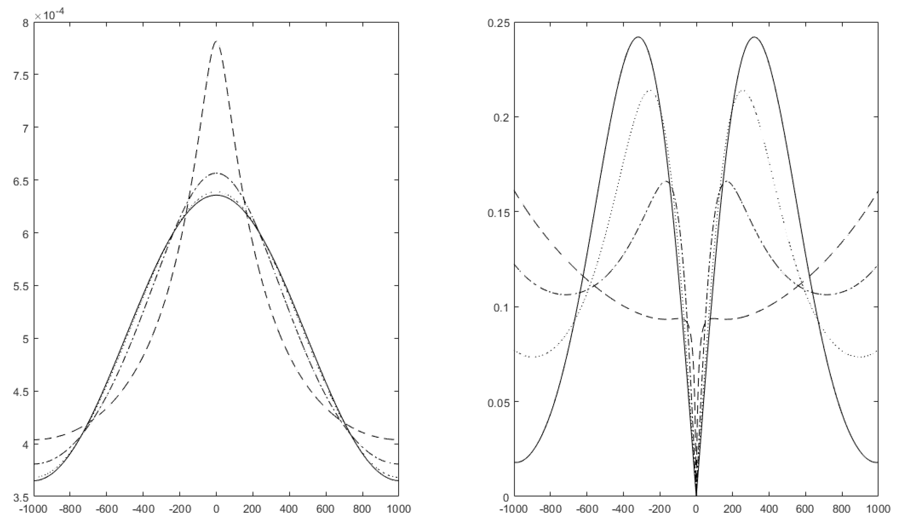
13.6. Discussion: Impulse Response Functions for Classical and Fractional Diffusion

Given Equation (43), it is clear that, in the asymptotic limit $x\to 0$, the difference between classical and fractional diffusion is compounded in the different Green’s function given by Equations (42) and (44). Thus, ignoring the scaling parameters in Equations (42) and (44) as well as those of their Fourier transforms, we can compare the asymptotic solutions as follows:

• Classical Diffusion

  $$u\left(t\right)=\frac{1}{\sqrt{t}}\otimes s\left(t\right),t>0\Rightarrow \mid U\left(\omega \right)\mid =\frac{\mid S\left(\omega \right)\mid }{\sqrt{\mid \omega \mid }}$$

  (46)
• Fractional Diffusion

  $$u\left(t\right)=\frac{1}{t^{1-1/\gamma }}\otimes s\left(t\right),t>0\Rightarrow \mid U\left(\omega \right)\mid =\frac{\mid S\left(\omega \right)\mid }{\mid \omega {\mid }^{1/\gamma }},\gamma \in [1,2]\Rightarrow D\in [1.5,2]$$

  (47)

Unlike classical diffusion, fractional diffusion is characterised by a range of values of the Lévy index. The efficient market hypothesis is predicated on classical diffusion processes, based on E${}^3$ for a Gaussian distribution. The ramifications of this is that the time series model for $u(0,t)$ given by Equation (46) is characterised by the impulse response function (IRF) $1/\sqrt{t}$. By comparison, the fractal market hypothesis is predicated on fractional diffusion processes based on E${}^3$ for a Lévy distribution. The consequence of this is that the time series model for $u(0,t)$ given by Equation (47) is characterised by the IRF $1/t^{1-1/\gamma }$. Since financial signals tend to be non-stationary random fractals, variations in $\gamma$ as a function of time are informative. However, before we study this, we consider another way to derive what is, in effective, the same basic result but via a different approach, an approach that is also based on E${}^3$ but obtained via the GKFE subject to application of an appropriate memory function. This is discussed in the following section.

14. Solution to the GKFE for an Orthonormal Memory Function

In this section, we show that the temporal power law which characterises Equation (43)—i.e., $1/t^{1-1/\gamma }$—can be obtained from Equation (14) for a specific orthonormal memory function. The purpose of this is to show another route to deriving the power law which is informative in that it is based on the application of a memory function alone and does not involve specific application of the FDE as presented in the previous section. In this case, and, for $\mathbf{r}\in {\mathbb{R}}^1$, by writing Equation (14) in the form

$$\tau \frac{\partial }{\partial t}u(x,t)+u(x,t)=u(x,t)-n\left(t\right)\otimes u(x,t)+n\left(t\right)\otimes u(x,t)\otimes p\left(x\right)$$

we can construct a Green’s function solution is given by

$$u(x,t)=g\left(t\right)\otimes u(x,t)-g\left(t\right)\otimes n\left(t\right)\otimes u(x,t)+g\left(t\right)\otimes n\left(t\right)\otimes u(x,t)\otimes p\left(x\right)$$

(48)

where $g\left(t\right)$ is the Green’s function given by

$$g\left(t\right)=\frac{1}{\tau }exp(-t/\tau ),t>0$$

which is the solution to

$$\tau \frac{\partial }{\partial t}g\left(t\right)+g\left(t\right)=\delta \left(t\right).$$

Provided the Laplace transform of the function $n\left(t\right)$ exists, we can write this Green’s function solution as

$$u(x,t)=h\left(t\right)\otimes u(x,t)\otimes p\left(x\right)$$

(49)

where

$$h\left(t\right)\leftrightarrow \frac{\overline{n}\left(s\right)}{\tau s+\overline{n}\left(s\right)}$$

and ↔ denotes the Laplace transformation, i.e., the mutual transformation from t-space to s-space. This result is obtained by using the convolution theorems for the Fourier and Laplace transforms, when Equation (14) can be written as

$$\overline{\tilde{u}}(k,s)=\overline{g}\left(s\right)\overline{\tilde{u}}(k,s)-\overline{g}\left(s\right)\overline{n}\left(s\right)\overline{\tilde{u}}(k,s)+\overline{g}\left(s\right)\overline{n}\left(s\right)\overline{\tilde{u}}(k,s)\tilde{p}\left(k\right)$$

where

$$\overline{\tilde{u}}(k,s)=\underset{0}{\overset{\infty }{\int }}\underset{-\infty }{\overset{\infty }{\int }}u(x,t)exp(-ikx)dxexp(-st)dt,\overline{g}\left(s\right)=\underset{0}{\overset{\infty }{\int }}g\left(t\right)exp(-st)dt,$$

$$\overline{n}\left(s\right)=\underset{0}{\overset{\infty }{\int }}n\left(t\right)exp(-st)dt\mathrm{and}\tilde{p}\left(k\right)=\underset{-\infty }{\overset{\infty }{\int }}p\left(x\right)exp(-ikx)dx$$

Thus, noting that $\overline{g}\left(s\right)={(1+\tau s)}^{-1}$, we can write

$$\overline{\tilde{u}}(k,s)=-\frac{\overline{g}\left(s\right)}{1-\overline{g}\left(s\right)}\overline{n}\left(s\right)\overline{\tilde{u}}(k,s)+\frac{\overline{g}\left(s\right)}{1-\overline{g}\left(s\right)}\overline{n}\left(s\right)\overline{\tilde{u}}(k,s)\tilde{p}\left(k\right)=-\frac{\overline{n}\left(s\right)}{\tau s}\overline{\tilde{u}}(x,t)+\frac{\overline{n}\left(s\right)}{\tau s}\overline{\tilde{u}}(k,s)\tilde{p}\left(k\right)$$

leading to the equation

$$\overline{\tilde{u}}(k,s)=\overline{h}\left(s\right)\overline{\tilde{u}}(k,s)\tilde{p}\left(k\right).$$

Inverse Fourier-Laplace transformation then gives Equation (49).

Equation (49) supports an iterative solution of the form

$$u_{m+1}(x,t)=h\left(t\right)\otimes u_m(x,t)\otimes p\left(x\right),m=0,1,2,\dots$$

and we may therefore consider an approximation based on the first iterate, i.e.,

$$u(x,t)=h\left(t\right)\otimes u_0(x,t)\otimes p\left(x\right)$$

The condition required for this approximation to apply can be obtained as follows: Given that

$${\parallel u(x,t)\parallel }_1\le {\parallel h\left(t\right)\parallel }_1\parallel u_0{(x,t)\parallel }_1{\parallel p\left(x\right)\parallel }_1={\parallel h\left(t\right)\parallel }_1{\parallel u_0(x,t)\parallel }_1$$

then

$$\frac{{\parallel u(x,t)\parallel }_1}{\parallel u_0{(x,t)\parallel }_1}\le {\parallel h\left(t\right)\parallel }_1$$

and hence we required that

$${\parallel h\left(t\right)\parallel }_1<<1.$$

(50)

Further, if we consider the case when $u_0(x,t)=\delta \left(x\right)s\left(t\right)$, then we can write

$$u\left(t\right)=\underset{-\infty }{\overset{\infty }{\int }}u(x,t)dx=h\left(t\right)\otimes s\left(t\right)\underset{-\infty }{\overset{\infty }{\int }}p\left(x\right)dx=h\left(t\right)\otimes s\left(t\right).$$

If we now choose a memory function $m\left(t\right)$ whose Laplace transform is $s^{\beta -1}$ then the orthonormality property $n\left(t\right)\otimes m\left(t\right)=\delta \left(t\right)$ is satisfied if the Laplace transform of $n\left(t\right)$ is $s^{1-\beta }$ given that from the convolution theorem for Laplace transforms $\overline{n}\left(s\right)\overline{m}\left(s\right)=1$. In this case

$$\overline{h}\left(s\right)=\frac{s^{1-\beta }}{\tau s+s^{1-\beta }}=\frac{1}{1+\tau s^{\beta }}\sim \frac{1}{\tau s^{\beta }},\tau >>1.$$

Since

$$\frac{1}{s^{\beta }}\leftrightarrow \frac{H\left(t\right)}{\Gamma \left(\beta \right)t^{1-\beta }}$$

we obtain the solution

$$u\left(t\right)=h\left(t\right)\otimes s\left(t\right)$$

where

$$h\left(t\right)=\frac{1}{\tau \Gamma \left(\beta \right)t^{1-\beta }},t>0.$$

This solution is characterised by Riemann–Liouville (fractional) integral which has self-affine properties, i.e., properties that exhibit “stochastic trending characteristics”. In other words, $u\left(t\right)$ defines a random scaling fractal function whose impulse response function is $1/t^{1-\beta }$, a result that is, in light of the above analysis, been shown to be a PDF independent first order solution to the GKFE for a memory function

$$m\left(t\right)=\frac{1}{\Gamma (1-\beta )t^{\beta }}.$$

In order to comply with Condition (50), we require that

$${\parallel h\left(t\right)\parallel }_1=\frac{1}{\tau \Gamma \left(\beta \right)}\underset{0}{\overset{\tau }{\int }}\frac{1}{t^{1-\beta }}=\frac{1}{\beta \Gamma \left(\beta \right){\tau }^{1-\beta }}<<1,$$

which is satisfied for the case when $\tau >>1,\beta \in [0,1)$.

Clearly, ignoring differences in scaling, compatibility of this solution for $u\left(t\right)$ with Equation (43) is obtained when $\beta =1/\gamma$. Thus, subject to the conditions imposed in each case we have shown that there exist temporal solutions to the FDE and the GKFE that exhibit a fundamental power law of $1/t^{1-1/\gamma }$ for Lévy index $\gamma$. In the former case, the solution is predicated on defining the PDF in the evolution equation (a Lévy distribution) whereas in the latter case, the result is independent of the PDF but predicated on the definition of the memory function (with power law $1/t^{\beta }$). In both cases, the solution is characterised by a fractional integral which is self-affine, a property that is fundamental to the analysis and interpretation of financial signals and underpins the fractal market hypothesis.

15. Time Varying Lévy- and $\alpha$-Indices

As with the other indices considered in this paper, the time dependence of $\gamma$ for a financial signal can be obtained by computing it over a moving (look-back) window. Figure 13 shows an example of this short time signature. for a financial signal (the first 1000 elements of the FTSE 100 prices given in Figure 3), normalised for display purposes. In this example $\gamma$ has been computed using the function given in Appendix A.7.

This result assumes that the short-time amplitude spectrum adheres to the scaling law $\mid \omega {\mid }^{-\frac{1}{\gamma }}$, and, strictly within the context of this spectral model, the numerical range of $\gamma$ is only limited by the original definition of the of a Lévy distribution, i.e.,  $\gamma \in [0,2]$ as given in Equation (17). The statement $\gamma \in (1,2]$ given in Equation (47) is a result of imposing the condition that $0<1/\gamma <1$ in order that the Fourier transform pair relationship given by Equation (3) is satisfied. However, if we arbitrarily consider a modified IRF given by $1/t^{1-1/\gamma },\gamma \in [0,2]$, then it is clear that we can consider a short time scaling function given by (for $t>0$)

$$u\left(t\right)=t^{\alpha }\mathrm{where}\left\{\begin{array}{cc}\alpha >0,\hfill & \gamma <1;\hfill \\ \alpha =0,\hfill & \gamma =1;\hfill \\ \alpha <0,\hfill & \gamma >1.\hfill \end{array}\right.$$

for the case when $s\left(t\right)=\delta \left(t\right)$. This result has similar properties to the Lyapunov exponent in terms of providing an ‘$\alpha$-index’ that reflects up-ward (for $\alpha >0$) and down-ward (for $\alpha <0$) trends. Further, as with the LVR considered in Section 10 and compounded in Equation (26) we can scale the $\alpha$-index by the inverse of the volatility to produce Alpha-to-volatility ratio (AVR) index given by

$${\alpha }_{\sigma }=\frac{\alpha }{\sigma }$$

(51)

In practice, the value of the $\alpha$ can easily be computed using the LSM which is compounded in the function Alpha given in Appendix A.8.

Following the same procedure to that discussed in Section 10.4 (specifically Figure 7), Figure 14 shows example results of running Backtester for the first 1000 elements of the FTSE 100 prices given in Figure 3 but for the AVR index ${\alpha }_{\sigma }\left[n\right]$ instead of ${\lambda }_{\sigma }\left[n\right]$. The example given is for Backtester (30,10,1000) which yields a combined entry/exit (long/short) accuracy of 60.98%. Note that this results is obtained by replacing the code

• L(m)=Lyapunov(s,T,1);%Compute the Lyapunov Exponent.
• V(m)=Volatility(s,T);%Compute the Volatility.
• R(m)=L(m)/V(m);%Compute the Lyapunov to Volatility Ratio (LVR).

with

• A(m)=Alpha(s,T);%Compute the Alpha Index.
• V(m)=Volatility(s,T);%Compute the Volatility.
• R(m)=A(m)/V(m);%Compute the Alpha-To-Volatility Ratio (AVR).

in function Backtester given in Appendix A.6.

Apart from the scale in amplitude, the signature of the ARV is very similar to the LVR (comparing Figure 14 and Figure 7). However, the trend prediction accuracy is relatively low and the computational time greater (due to the repeated application of the LSM) which suggests that the LVR is a more reliable and computationally efficient index. However, this statement must be understood within the context of the limited data that was used and demonstrated for this publication and must be quantified further using $WT$-maps for a range of financial signals and the functions given in Appendix A, a study that lies beyond the scope of this work.

16. Summary, Conclusions and Open Questions

One of the principal themes of this paper has been to develop financial indices that in all cases can been traced back to a fundamental field equation of statistical physics, namely, Einstein’s evolution equation—Equation (10). In this context, we have developed expressions for the following financial indices:

• the Lyapunov Exponent;
• the Volatility;
• the Lévy Index.

16.1. Summary

We have explored the ability for the time varying Lyapunov-to-volatility ratio (LVR) to predict the trend of a financial signal in terms of a change in polarity and the period over which that polarity is sustained subject to pre- and post-filtering as discussed in Section 10.1.1 and Section 10.1.2, respectively. The filtering processes are critically dependent on the values of the look-back windows that are applied and a quantification of the values required to optimise the predictive power has been explored in Section 10.4 in terms of the $WT$ map. Application of the LVR provides a time signature whose maximum and minimum values correlate with regions of a financial signal that have up-ward and down-ward trends with low volatility, respectively. In Section 11, a short study has been presented to use this result as a criterion for the application of EC to predict short term future prices. In this context, computing the time varying LVR has two primary uses:

• predicting the entry points in time for making, holding or withdrawing an investment;
• assessing the position in time when application of EC can be expected to yield optimally accurate short term price predictions.

It is noted that in regard to the application of EC, the volatility alone can be used as an assessment criterion, low volatilities providing a flag for the use of EC on a moving window basis to update previous price predictions.

While the derivation and the application of the LVR is predicated on the evolution equation (at least, as demonstrated in this paper), it does not rely on the application of fractional calculus which has been a focal issue in regard to the composition of this paper. Thus, the latter half of this paper was devoted to an analysis of fractional calculus with the aim of showing how, in particular, the classical diffusion and fractional diffusion equations are both directly related to the evolution equation and can be derived directly from it, the difference between the two equations being compounded in the PDF that "governs" the spatial distribution of the density field.

We have shown that the classical diffusion equation is predicated on a Gaussian distribution and that the fractional diffusion equation is predicated on a (symmetric) Lévy distribution. In turn, it has been shown that at the spatial origin (i.e., as $x\to 0$), the temporal impulse response functions for these two cases are given by $1/\sqrt{t}$ and $1/t^{1-1/\gamma }$, respectively, functions that underpin the efficient and fractal market hypotheses, respectively. In deriving these functions, we have attempted to show the intrinsic connectivity between the application of Lévy statistics to the evolution equation, the fractional diffusion, the application of fractional calculus for solving this equation and the analysis of the solution leading directly to the description of a stochastic self-affine field—a random scaling fractal signal.

In addition to the theoretical concepts presented in this paper, we have provided a set of numerical algorithms that allows the reader to reproduce the results given. These algorithms are based on the m-code given in Appendix A. They have been designed to give interested readers the facility to study the methods used for the wide variety of financial time series available online and to develop the algorithms further as required. Their development has been based on maintaining consistency with the theoretical analysis derived at the expense of any further and more sophisticated software engineering. Hence, issues such as error checks on input/output data, processing parameters and data/processor compatibility have not been considered.

16.2. Conclusions

The application of fractional calculus in mathematical finance is well known and in this paper we have provided a unified approach to showing that this is the case using Einstein’s evolution equation as a fundamental field equation. This approach has the potential for the development of a range of new models for a financial signal by introducing different PDFs in Equation (11) to those that have been considered here, the categorisation of such models for different time series lying beyond the scope of this publication.

The primary results are given in Section 10 which shows that a relatively high accuracy for predicting up-ward and down-ward trends can be obtained, thereby providing the potential for a profitable trading strategy to be implemented. However, it must be noted that the quantitative results given in Section 10 in regard to this statement are strictly applicable only to the data used (i.e., the daily FTSE100 and Euro-USA dollar exchange rate). Application of the algorithms presented must therefore be fully quantified and characterised for any and all specific financial time series data used, "quantification" being compounded in the associated $WT$ map.

The use of EC discussed in Section 11 verifies that short time price prediction can be exercised if the LVR has reached a maximum or minimum threshold in excess of +2 or $-2$, respectively. However, as pointed out in Section 11, the material presented in this respect has only been introduced to complement the main theme of this paper. Further studies are required to assess the accuracy of EC prediction on a moving window basis in terms of the number of future projected price values which maintain an appropriate forecasting accuracy and the associated look-back window used to generate short time forecasting equations of the type given by Equation (27), for example.

16.3. Open Questions

There are a number of open questions which this paper has raised that are the subject of further investigation. The reader is invited to consider the following examples:

• The specific form of the evolution equation used in this work has been based on Equation (11) and it may be of value to consider the affect of the decay term $-Ru(\mathbf{r},t)$ given in Equation (12).
• Given that the critical step in deriving the IRF $1/t^{1-1/\gamma }$ (from which $\gamma$ can be computed) is the asymptotic condition $x\to 0$, what are the consequences of developing a numerical algorithm to compute $\gamma$ when this condition is negated?
• What is the impact of the LVR and AVR in terms of their possible inclusion into machine learning algorithms that use sets of more conventional financial indices and other statistical metrics for forecasting?

In regard to more generic questions, the following examples may be of interest:

• In regard to E${}^3$, the PDFs considered in this work are the delta function, Gaussian function and Lévy distribution which provide models associated with the random walk, efficient and fractal hypothesis, respectively. An investigation into the models for $u(\mathbf{r},t)$ and metrics thereof, associated with the application of different PDF (including non-symmetric distributions), is therefore warranted.
• Similarly, what is the effect of introducing different memory functions into the generalised Kolmogorov–Feller equation, i.e., E${}^3$ in all but name, expressed in terms of memory function $m\left(t\right)$, and, further, is it possible to develop an inverse solution in which a financial signal $u\left(t\right)$ can be used to derive a estimate of $m\left(t\right)$ for a known distribution $p\left(\mathbf{r}\right)$.
• What is the relationship/connectivity (or otherwise) between fractional and Itô calculus in regard to E${}^3$?

16.4. Final Remarks

One of the primary aims of this paper was to realise the connectivity compounded in Table 1, and, in this broader context, to show the relationship between E${}^3$ and fractional calculus through the application of a non-Gaussian distribution, specifically a symmetric Lévy distribution whose characteristic function is a generalisation of the Gaussian function (for a real constant c) $exp(-c\mid k{\mid }^2)$ to $exp(-c\mid k{\mid }^{\gamma }),0<\gamma <2$. The effect of this has been to show that there is a close relationship between non-Gaussian processes of this type and the self-affine characteristics of stochastic signals modelled in terms of the solution to a fractional differential equation, i.e., the fractional diffusion equation. This approach provides the basis for a more general study that transcends the specific distributions considered in order to derive stochastic models that are a more complete and accurate description associated with the varied properties of financial signals in which the applications of fractional calculus is a central theme.

In terms of the computational methods presented, a primary aim is to classify the $WT$ maps for a range of different financial data in terms of the LVR and AVR and to further quantify the accuracy of these two indices in regard to different data types. The purpose of this is to categorise the type of financial times series that are best suited to the trend analysis proposed in terms of a robust predictive accuracy. In turn, this exercise will inform a quantification of the use of EC for predicting short term prices with the aim of obtain a quantitative relationship between the look-back window used, the number of future prices that can be predicted with a specified accuracy and the amplitude of the LVR and/or ALR for a specific financial signal.

References

1. Einstein, A. On the Motion of Small Particles Suspended in Liquids at Rest Required by the Molecular-Kinetic Theory of Heat. Annalen der Physik 1905, 17, 549–560. [Google Scholar] [CrossRef]
2. Navarro, L. Gibbs, Einstein and the Foundations of Statistical Mechanics. Arch. Hist. Exact Sci. 1998, 53, 147–180. [Google Scholar] [CrossRef]
3. Tindel, S.; Tudor, C.A.; Viens, F. Stochastic Evolution Equations with Fractional Brownian Motion. Probab. Theory Relat. Fields 2003, 127, 186–204. [Google Scholar] [CrossRef]
4. Peters, E.E. Fractal Market Analysis: Applying Chaos Theory to Investment and Economics; Wiley Finance; Wiley: Hoboken, NJ, USA, 1994; ISBN-13 978-0471585244. [Google Scholar]
5. Blackledge, J.M. The Fractal Market Hypothesis: Applications to Financial Forecasting; Lecture Notes Series 4; Centre for Advanced Studies; Polish Academy of Sciences: Warsaw, Poland, 2010; ISBN 978-83-61993-01-8. [Google Scholar]
6. Blackledge, J.M.; Lamphiere, M.; Murphy, K.; Overton, S. Financial Forecasting using the Kolmogorov-Feller Equation. In AENG Transactions on Engineering Technologies: Special Volume of the World Congress on Engineering 2012; Lecture Notes in Electrical Engineering; Yang, G.-C., Ao, S.-L., Gelman, L., Eds.; Springer: Berlin/Heidelberg, Germany, 2013; Volume 229, ISBN 978-94-007-6190-2. [Google Scholar]
7. Blackledge, J.M.; Lamphiere, M.; Murphy, K.; Overton, S. Stochastic Volatility Analysis using the Generalised Kolmogorov-Feller Equation. In Proceedings of the International Conference of Financial Engineering, World Congress on Engineering (WCE2012), London, UK, 4–6 July 2012; pp. 453–458. [Google Scholar]
8. Blackledge, J.M. A New Forex Currency Exchange Indicator. In European Success Stories in Industrial Mathematics; Springer: Berlin/Heidelberg, Germany, 2011; p. 131. ISBN 978-3-642-23847-5. [Google Scholar]
9. Blackledge, J.M.; Murphy, K. Forex Trading Using MetaTrader4 with the Fractal Market Hypothesis, Risk Management Trends; Giancarlo, N., Ed.; InTech Publishing: London, UK, 2011; pp. 129–146. ISBN 978-953-307-154-1. [Google Scholar]
10. Blackledge, J.M. Application of the Fractal Market Hypothesis for Modelling Macroeconomic Time Series. ISAST Trans. Electron. Signal Process. 2008, 2, 89–110. [Google Scholar]
11. Blackledge, J.M. Application of the Fractional Diffusion Equation for Predicting Market Behaviour. IAENG Int. J. Appl. Math. 2010, 40, 130–158. [Google Scholar]
12. Blackledge, J.M.; Rebow, M. Economic Risk Assessment using the Fractal Market Hypothesis. In Proceedings of the 5th International Conference on Internet Monitoring and Protection, Valencia, Spain, 22–26 May 2010; pp. 41–47. [Google Scholar]
13. Blackledge, J.M.; Murphy, K. Forex Trading using MetaTrader 4 with the Fractal Market Hypothesis. In Proceedings of the Third International Conference on Resource Intensive Applications and Services, INTENSIVE 2011, Venice, Italy, 22–27 May 2011; pp. 1–9, ISBN 978-1-61208-006-2. [Google Scholar]
14. Blackledge, J.M.; Murphy, K. Predicting Currency Pair Trends using the Fractal Market Hypothesis. In Proceedings of the IET ISSC2011, Dublin, Ireland, 23–24 June 2011. [Google Scholar]
15. The Fourier Transform, Tables of Important Fourier Transforms. Wikipedia. 2019. Available online: https://en.wikipedia.org/wiki/Fourier_transform (accessed on 23 July 2019).
16. Podlubny, I. Geometric and Physical Interpretation of Fractional Integration and Fractional Differentiation. Fract. Calc. Appl. Anal. 2002, 5, 367–386. [Google Scholar]
17. Tavassoli, M.H.; Tavassoli, A.; Ostad Rahimi, M.R. The Geometric and Physical Interpretation of Fractional Order Derivatives of Polynomial Functions. Differ. Geom.-Syst. 2013, 15, 93–104. [Google Scholar]
18. Butera, S.; Di Paola, M. A Physically based Connection Between Fractional Calculus and Fractal Geometry. Ann. Phys. 2014, 350, 146–158. [Google Scholar] [CrossRef]
19. Kiryakova, V. Generalised Fractional Calculus and Applications; Longman: Harlow, UK, 1994. [Google Scholar]
20. Zheng, Z.; Zhao, W.; Dai, H. A New Definition of Fractional Derivative. Int. J. Non-Linear Mech. 2019, 108, 1–6. [Google Scholar] [CrossRef]
21. Hermann, R. Fractional Calculus: An Introduction for Physicists; World Scientific: Singapore, 2014. [Google Scholar]
22. Zhou, Y. Basic Theory of Fractional Differential Equations; World Scientific: Singapore, 2014. [Google Scholar]
23. Investing.com. 2019. Available online: https://uk.investing.com/indices/uk-100-historical-data (accessed on 2 August 2019).
24. Investopedia. 2019. Available online: https://www.investopedia.com (accessed on 24 July 2019).
25. Kolmogorov, A.N. On Analytic Methods in Probability Theory. In Selected Works of A.N. Kolmogorov, Volume II: Probability Theory and Mathematical Statistics; Shiryaev, A.N., Ed.; Kluwer: Dordrecht, The Netherlands, 1992; pp. 61–108, (Original: Uber die Analytischen Methoden in der Wahrscheinlichkeitsrechnung. Math. Ann. 1931, 104, pp. 415–458). [Google Scholar]
26. Feller, W. On Boundaries and Lateral Conditions for the Kolmogorov Differential Equations. Ann. Math. 1957, 65, 527–570. [Google Scholar] [CrossRef]
27. Bachelier, L. Théorie de la spéculation. Annales Scientifiques de l’École Normale Supérieure 1900, 3, 21–86. [Google Scholar] [CrossRef]
28. Working, H. A Random-Difference Series for Use in the Analysis of Time Series. J. Am. Stat. Assoc. 1934, 29, 11–24. [Google Scholar] [CrossRef]
29. Kendall, M.G.; Bradford Hill, A. The Analysis of Economic Time-Series-Part I: Prices. J. R. Stat. Soc. Ser. A 1953, 116, 11–34. [Google Scholar] [CrossRef]
30. Fama, E.F. Efficient Capital Markets: A Review of Theory and Empirical Work. J. Financ. 1970, 25, 383–417. [Google Scholar] [CrossRef]
31. Campbell, J.Y.; Lo, A.W.; Mackinlay, A.C. The Econometrics of Financial Markets; Princeton University Press: Princeton, NJ, USA, 1996. [Google Scholar]
32. Sewell, M. History of the Efficient Market Hypothesis, Research Not RN/11/04. UCL Department of Computer Science. 2011. Available online: http://www.cs.ucl.ac.uk/fileadmin/UCL-CS/images/Research_Student_Information/RN_11_04.pdf (accessed on 6 July 2019).
33. Investopedia. 2019. Available online: https://www.investopedia.com/terms/b/blackscholes.asp (accessed on 25 July 2019).
34. Elliott, R.N. The Wave Principle. Amazon. 2012. Available online: https://www.amazon.co.uk/Wave-Principle-Ralph-Nelson-Elliott/dp/1607964961 (accessed on 28 July 2019).
35. Frost, A.J.; Prechter, R.R. Amazon 2017. Available online: https://www.amazon.co.uk/Elliott-Wave-Principle-Market-Behavior/dp/1616040815 (accessed on 28 July 2019).
36. WolframAlpha Computational Intelligence. 2019. Available online: https://www.wolframalpha.com/input/?i=Fourier+transform (accessed on 28 July 2019).
37. Blackledge, J.M.; Rani, T.R. Stochastic Modelling for Lévy Distributed Systems. Math. Aeterna 2017, 7, 193–210. [Google Scholar]
38. Blackledge, J.M. Digital Signal Processing, 2nd ed.; Horwood Publishing: Cambridge, UK, 2006; p. 418. ISBN 1-904275-26-5. Available online: https://arrow.dit.ie/engschelebk/4/ (accessed on 19 June 2019).
39. Bryant, P.; Brown, R.; Abarbanel, H. Lyapunov Exponents From Observed Time Series. Phys. Rev. Lett. 1990, 65, 1523–1526. [Google Scholar] [CrossRef]
40. Brown, R.; Bryant, P.; Abarbanel, H. Computing the Lyapunov Spectrum of a Dynamical System From an Observed Time Series. Phys. Rev. A 1991, 43, 2787–2806. [Google Scholar] [CrossRef]
41. Abarbanel, H.; Brown, R.; Kennel, M.B. Local Lyapunov Exponents Computed from Observed Data. J. Nonlinear Sci. 1992, 2, 343–365. [Google Scholar] [CrossRef]
42. Eiben, A.E.; Schoenauer, M. Evolutionary Computing. Inf. Process. Lett. 2002, 82, 1–6. [Google Scholar] [CrossRef]
43. Fogel, L.J.; Owens, A.J.; Walsh, M.J. Artificial Intelligence through Simulated Evolution; Wiley: Hoboken, NJ, USA, 1966. [Google Scholar]
44. Holland, J.H. Adaptation in Natural and Artificial Systems: An Introductory Analysis with Applications to Biology, Control, and Artificial Intelligence; University of Michigan Press: Ann Arbor, MI, USA, 1975. [Google Scholar]
45. Rechenberg, I. Evolutionsstrategien, Simulationsmethoden in der Medizin und Biologie; Springer: Berlin/Heidelberg, Germany, 1978; pp. 83–114. [Google Scholar]
46. Eiben, A.E.; Smith, J.E. Introduction to Evolutionary Computing; Springer: Berlin/Heidelberg, Germany, 2003. [Google Scholar]
47. Schmidt, M.; Lipson, H. Eureqa. 2014. Available online: www.nutonian.com (accessed on 23 August 2019).
48. Schmidt, M.; Lipson, H. Distilling Free-form Natural Laws from Experimental Data. Science. 2009. Available online: https://science.sciencemag.org/content/324/5923/81 (accessed on 24 August 2019).
49. Dubcakova, R. Eureqa: Software Review. Genet. Program. Evolvable Mach. 2011, 12, 173–178. [Google Scholar] [CrossRef]
50. Ehrenberg, R. Software Scientist: With a Little Data, Eureqa Generates Fundamental Laws of Nature’. Sci. News 2012, 181, 20–21. [Google Scholar] [CrossRef]
51. Abbott, R. Equity Markets and Computational Intelligence. In Proceedings of the 2010 UK Workshop on Computational Intelligence (UKCI), Colchester, UK, 8–10 September 2010; pp. 1–6. [Google Scholar]
52. Walsh, P. An Econophysics Approach to the Trading of Energy Commodities. Ph.D. Thesis, Technological University Dublin, Dublin, Ireland, 2018. [Google Scholar]
53. Wheelwright, S.C.; Makridakis, S.G. Forecasting Nethods for Management; Wiley: Hoboken, NJ, USA, 1973. [Google Scholar]
54. Evans, G.; Blackledge, J.M.; Yardley, P. Analytic Solutions to Partial Differential Equations; Springer: Berlin/Heidelberg, Germany, 1999. [Google Scholar]
55. Crack, T.F. Basic Black-Scholes: Option Pricing and Trading; Amazon: Seattle, WA, USA, 2017; ISBN-13 978-0994138682. [Google Scholar]
Figure 1. Simulation of a financial signal based on the sum of independent random walks; basis for the Random Walk Hypothesis.
Mathematics 07 01057 g001
Figure 2. Left: Lévy distributions p ( x ) for γ = 2 (solid line), γ = 1.5 (dotted line), γ = 1 (dot-dashed line), and γ = 0.5 (dashed line) for c = 2 ; Right: Plots of associated distributions x p ( x ) for γ = 2 (solid line), γ = 1.5 (dotted line), γ = 1 (dot-dashed line) and γ = 0.5 (dashed line) for c = 1 / 2 .
Mathematics 07 01057 g002
Figure 3. Example of Lévy flights. Left: Plot of the FTSE100 daily prices from 14/03/2006 to 12/04/2019— u ( t ) ; Right: Complex plane plot of s ( t ) given by Equation (16). Both time functions u ( t ) and s ( t ) are taken to be uniformly sampled discrete functions u n and s n , respectively; the analytic signal is computed using a fast Fourier transform (FFT) and the algorithm presented in [38].
Mathematics 07 01057 g003
Figure 4. Example of computing the time varying Lyapunov exponent (lower signal) for a financial signal (upper signal after normalisation) through application of Equation (23) for a look-back window of size N = 32 and with τ = 0.01 .
Mathematics 07 01057 g004
Figure 5. Example of computing the time dependent volatility (lower signal) using Equation (25) for a normalised financial signal (upper signal) with a look-back window of N = 32 .
Mathematics 07 01057 g005
Figure 6. Example of computing the time dependent LVR λ σ (solid line —) for a normalised financial signal (bold solid line —) with a look-back window of N = 32 .
Mathematics 07 01057 g006
Figure 7. Example graphical outputs from function Backtester. Each plot shows the post-filtered (for T = 10 ) LVR λ σ [ n ] (dotted line), the pre-filtered time series u n after normalisation (dot-dashed line) and z c [ n ] (solid line) which identifies the zero-crossings of λ σ [ n ] . The plots provided are for the case when pre-filtering is undertaken for look-back window sizes of W = 10 (top), W = 20 (centre) and W = 30 (lower plot). The financial time series data used in this case is the FTSE100 daily prices from 14/03/2006 to 26/02/2010.
Mathematics 07 01057 g007
Figure 8. Surface (mesh) plot of the combined long/short predictive accuracy as a function of the pre- and post-filtering look-back window sizes W and T, respectively, for FTSE100 daily prices from 14/03/2006 to 26/02/2010.
Mathematics 07 01057 g008
Figure 9. Surface (mesh) plot of the combined long/short predictive accuracy as a function of the pre- and post-filtering look-back window sizes W and T, respectively, for Eruo-Dollar (USA) daily (averaged) exchange rates from 29/04/2008 to 27/02/2012 as given in Figure 10.
Mathematics 07 01057 g009
Figure 10. Eruo-Dollar (USA) daily (averaged) exchange rates from 29/04/2008 to 27/02/2012.
Mathematics 07 01057 g010
Figure 11. FTSE 100 price values (dots) for 30 days between 24/08/2009 and 08/09/2009 (inclusively) and the estimate (solid line) obtained from the evolutionary computed formula given by Equation (28). The graph compares the actual prices (circled dots) and predicted future values for three days after 08/09/2009 using the same formula.
Mathematics 07 01057 g011
Figure 12. Examples of the function u n given by the discretised form of Equation (43) for γ = 1 / 2 , 1 , and 3 / 2 (left plots, respectively) and the associated complex plane representations obtained using Equation (16)—right plots, respectively.
Mathematics 07 01057 g012
Figure 13. Example of computing the time dependent Lévy index (solid line —) for a normalised financial signal (bold solid line ) based on the application of Equation (45) using function Levy with a look-back window of 50 data elements.
Mathematics 07 01057 g013
Figure 14. Example graphical output from function Backtester. The plot shows the post-filtered (for T = 10 ) AVR α σ [ n ] (dotted line), the pre-filtered time series u n (dot-dashed line) and z c [ n ] (solid line) which identifies the zero-crossings of α σ [ n ] . The plot is for the case when pre-filtering is undertaken for a look-back window size of W = 30 and post-filtering using a look-back window size of T = 10 . The financial time series data used in this case is FTSE100 daily prices: 14/03/2006–26/02/2010.
Mathematics 07 01057 g014