Computing the Matrix Exponential with an Optimized Taylor Polynomial Approximation

Abstract

A new way to compute the Taylor polynomial of a matrix exponential is presented which reduces the number of matrix multiplications in comparison with the de-facto standard Paterson-Stockmeyer method for polynomial evaluation. Combined with the scaling and squaring procedure, this reduction is sufficient to make the Taylor method superior in performance to Padé approximants over a range of values of the matrix norms. An efficient adjustment to make the method robust against overscaling is also introduced. Numerical experiments show the superior performance of our method to have a similar accuracy in comparison with state-of-the-art implementations, and thus, it is especially recommended to be used in conjunction with Lie-group and exponential integrators where preservation of geometric properties is at issue.

1. Introduction

Many differential equations arising in applications are most appropriately formulated as evolving on Lie groups or on manifolds acted upon Lie groups. Examples include fields such as rigid mechanics, Hamiltonian dynamics and quantum mechanics. In all these cases, it is of paramount importance that the corresponding approximations obtained when discretizing the equation also belong to the same Lie group. Only in this way are important qualitative properties of the continuous system inherited by the numerical approximations. For instance, in quantum mechanics, any approximation to the solution of the time-dependent Schrödinger equation has to evolve in the special unitary group, so as to guarantee that the total transition probability is preserved.

Lie-group methods are a class of numerical integration schemes especially designed for this task, since they render by construction numerical approximations evolving in the same Lie group as the original differential equation [1,2]. In this sense, they belong to the domain of geometric numerical integration [3,4]. Here one is not only concerned with the classical accuracy and stability of the numerical algorithm, but in addition, the method must also incorporate into its very formulation the geometric properties of the system. This gives the integrator not only an improved qualitative behavior, but also allows for a significantly more accurate long-time integration than is the case with general-purpose methods.

Geometric numerical integration has been an active area of research during the few last decades, and in fact, very efficient geometric integrators have been designed and applied in a variety of contexts where preserving qualitative characteristics is at issue. In the particular case of Lie-group methods, some of the most widely used are the Runge–Kutta–Munthe-Kaas family of schemes [2], and, in the case of explicitly time-dependent matrix linear ordinary differential equations, $Y^{\prime }=A(t,Y)Y$, integrators based on the Magnus expansion [5,6]. In both instances, the discrete approximation is obtained as the exponential of linear combination of nested commutators, and it is this feature which guarantees that the approximation rests in the relevant Lie group. There are also other families of Lie-group methods that do not involve commutators at the price of requiring more exponentials per step [7,8]. It is then, of prime importance to compute, numerically, the matrix exponential as accurately and as fast as possible to render truly efficient integrators.

Another class of schemes that have received considerable attention in the literature, especially in the context of stiff problems, is that formed by exponential integrators, both for ordinary differential equations and for the time-integration of partial differential equations [9]. For them, the numerical approximation also requires computing the exponential of matrices at every time step, and this represents, sometimes, a major factor in the overall computational cost of the method.

One is thus led, when considering these types of methods, to the problem of computing the matrix exponential in an efficient way, and this was precisely the goal of the present work. As a matter of fact, the search for efficient algorithms to compute the exponential of a square matrix has a long history in numerical mathematics, given the wide range of its applications in many branches of science. Its importance is clearly showcased by the great impact achieved by various reviews devoted to the subject, e.g., [10,11,12,13], and the variety of proposed techniques. Our approach here consists of combining the scaling and squaring procedure with an optimized way of evaluating the Taylor polynomial of the matrix exponential function. With the ensuing cost reduction, a method for computing $e^{hA}$, where h is the time step, is proposed using $2,3,4$ and 5 matrix-matrix products to reach accuracy up to $h^p$ for $p=4,8,12$ and 18, respectively. In combination with the scaling and squaring technique, this yields a procedure to compute the matrix exponential up to the desired accuracy at lower computational cost than the standard Padé method for a wide range of matrices $hA$. We also present a modification of the procedure designed to reduce overscaling that is still more efficient than state-of-the-art implementations. The algorithm has been implemented in Matlab and is recommended to be used in conjunction with Lie-group and exponential integrators where preservation of geometric properties is at issue. Moreover, although our original motivation for this work comes from Lie-group methods, it turns out that the procedure we present here can also be used in a more general setting where it is necessary to compute the exponential of an arbitrary matrix.

The plan of the paper is the following. In Section 2 we summarize the basic facts of the standard procedure based on scaling and squaring with Padé approximants. In Section 3, we outline the new procedure to compute matrix polynomials, reducing the number of matrix products, whereas in Section 4 we apply it to the Taylor polynomial of the exponential and discuss maximal attainable degrees at a given number of matrix multiplications. Numerical experiments in Section 5 show the superior performance of the new scheme when compared to a standard Padé implementation using scaling and squaring (cf. Matlab Release R2013a) (The MathWorks, Inc., Natick, MA, USA). Section 6 is dedicated to error estimates and adaptations to reduce overscaling along the lines of the more recent algorithms [14] (cf. Matlab from Release R2016a), including execution times of several methods. Finally, Section 7 contains some concluding remarks.

This work is an improved and expanded version of the preprint [15], where the ideas and procedures developed here were presented for the first time.

2. Approximating the Exponential

Scaling and squaring is perhaps the most popular procedure to compute the exponential of a square matrix when its dimensions runs well into the hundreds. As a matter of fact, this technique is incorporated in popular computing packages such as Matlab (expm) and Mathematica (MatrixExp) in combination with Padé approximants [10,14,16].

Specifically, for a given matrix $A\in {\mathbb{C}}^{N\times N}$, the scaling and squaring technique is based on the key property

$$e^A={\left(e^{A/2^s}\right)}^{2^s},s\in \mathbb{N}.$$

(1)

The exponential $e^{A/2^s}$ is then replaced by a rational approximation $r_m(A/2^s)$; namely, the $[m/m]$ diagonal Padé approximant to $e^x$. The optimal choice of both parameters, s and m, is determined in such a way that full machine accuracy is achieved with the minimal computational cost [14].

Diagonal $[m/m]$ Padé approximants have the form (see, e.g., [17] and references therein)

$$r_m(A)={\left[p_m(-A)\right]}^{-1}{p}_m(A),$$

(2)

where the polynomial $p_m(x)$ is given by

$$p_m(x)=\sum _{j=0}^m\frac{(2m-j)!m!}{(2m)!(m-j)!}\frac{x^j}{j!},$$

(3)

so that $r_m(A)=e^A+\mathcal{O}(A^{2m+1})$. In practice, the evaluation of $p_m(A),p_m(-A)$ is carried out trying to minimize the number of matrix products. For estimating the computational effort required, the cost of the inverse is taken as $4/3$ the cost of one matrix product. For illustration, the computation procedure for $r_5(A)$ is given by [10]

$$\begin{array}{cc}\hfill & u_5=A\left(b_5{A}_4+b_3{A}_2+b_{1}I\right),\hfill \\ \hfill & v_5=b_4{A}_4+b_2{A}_2+b_{0}I,\hfill \\ \hfill & (-u_5+v_5)r_5(A)=u_5+v_5\hfill \end{array}$$

(4)

with appropriate coefficients $b_j$, whereas for $r_{13}(A)$, one has

$$\begin{array}{cc}\hfill & u_{13}=A\left(A_6\left(b_{13}{A}_6+b_{11}{A}_4+b_9{A}_2\right)+b_7{A}_6+b_5{A}_4+b_3{A}_2+b_{1}I\right),\hfill \\ \hfill & v_{13}=A_6\left(b_{12}{A}_6+b_{10}{A}_4+b_8{A}_2\right)+b_6{A}_6+b_4{A}_4+b_2{A}_2+b_{0}I,\hfill \\ \hfill & (-u_{13}+v_{13})r_{13}(A)=u_{13}+v_{13}.\hfill \end{array}$$

(5)

Here $A_2=A^2$, $A_4=A_2^2$ and $A_6=A_2{A}_4$. Written in this form, it is clear that only three and six matrix multiplications and one inversion are required to obtain approximations of order 10 and 26 to the exponential, respectively. Diagonal Padé approximants $r_m(A)$ with $m=3,5,7,9$ and 13 are used, in fact, by the function expm in Matlab.

In the implementation of the scaling and squaring algorithm, the choice of the optimal order of the approximation and the scaling parameter for a given matrix A are based on the control of the backward error [10]. More specifically, given an approximation $t_n(A)$ to the exponential of order n, i.e., $t_n(A)=e^A+\mathcal{O}(A^{n+1})$, if one defines the function $h_{n+1}(x)=log(e^{-x}{t}_n(x))$, then $t_n(2^{-s}A)=e^{2^{-s}A+h_{n+1}(2^{-s}A)}$ and

$${\left(t_n(2^{-s}A)\right)}^{2^s}=e^{A+2^s{h}_{n+1}(2^{-s}A)}\equiv e^{A+\Delta A},$$

where $\Delta A=2^s{h}_{n+1}(2^{-s}A)$ is the backward error originating in the approximation of $e^A$. If in addition $h_{n+1}$ has a power series expansion

$$h_{n+1}(x)=\sum _{k=n+1}^{\infty }{c}_k{x}^k$$

with radius of convergence $\omega$, then it is clear that $\parallel h_{n+1}(A)\parallel \le {\tilde{h}}_{n+1}(\parallel A\parallel )$, where

$${\tilde{h}}_{n+1}(x)=\sum _{k=n+1}^{\infty }\left|c_k\right|x^k,$$

and thus

$$\frac{\parallel \Delta A\parallel }{\parallel A\parallel }=\frac{\parallel h_{n+1}(2^{-s}A)\parallel }{\parallel 2^{-s}A\parallel }\le \frac{{\tilde{h}}_{n+1}(\parallel 2^{-s}A\parallel )}{\parallel 2^{-s}A\parallel }.$$

(6)

Given a prescribed accuracy u (for instance, $u=2^{-53}\simeq 1.1\times {10}^{-16}$, the unit roundoff in double precision), one computes

$${\theta }_n=max\{\theta :{\tilde{h}}_{n+1}(\theta )/\theta \le u\}.$$

(7)

Then, $\parallel \Delta A\parallel \le u\parallel A\parallel$ if s is chosen so that $\parallel 2^{-s}A\parallel \le {\theta }_n$ and ${\left(t_n(2^{-s}A)\right)}^{2^s}$ is used to approximate $e^A$.

In the particular case that $t_n$ is the $[m/m]$ diagonal Padé approximant $r_m$, then $n=2m$, and the values of ${\theta }_{2m}$ are collected in

Table 1. Values of ${\theta }_{2m}$ for the diagonal Padé approximant $r_m$ of order $2m$ with the minimum number of products $\pi$ for single and double precision. In bold, we have highlighted the asymptotically optimal order at which it is advantageous to apply scaling and squaring since the increase of $\theta$ per extra product is smaller than the factor 2 from squaring. The values for double precision are taken from ([16], Table A.1).

$\pi :$	0	1	2	3	4	5	6
2m:	2	4	6	10	14	18	26
$u\le 2^{-24}$	$8.46\times {10}^{-4}$	$8.09\times {10}^{-2}$	$4.26\times {10}^{-1}$	1.88	$\mathbf{3.93}$	6.25	11.2
$u\le 2^{-53}$	$3.65\times {10}^{-8}$	$5.32\times {10}^{-4}$	$1.50\times {10}^{-2}$	$2.54\times {10}^{-1}$	$9.50\times {10}^{-1}$	2.10	$\mathbf{5.37}$

when u is the unit roundoff in single and double precision for $m=1,2,3,5,7,9,13$. According to Higham [10], $m=13$ and therefore $r_{13}$, is the optimal choice in double precision when scaling is required. When $\parallel A\parallel \le {\theta }_{26}$, the algorithm in [10] takes the first $m\in \{3,5,7,9,13\}$ such that $\parallel A\parallel \le {\theta }_{2m}$. This algorithm is later referred to as expm2005.

Padé approximants of the form (2) are not, of course, the only option one has in this setting. Another approach to the problem consists of using the Taylor polynomial of degree m as the underlying approximation $T_n$ to the exponential; i.e., taking $T_m(A)={\sum }_{k=0}^m{A}^k/k!$ computed in an efficient way.

Early attempts for efficiently evaluating matrix Taylor polynomials trace back to the work by Paterson and Stockmeyer [18]. When $T_m(A)$ is computed according to the Paterson-Stockmeyer (P-S) procedure, the number of matrix products is reduced and the overall performance is improved for matrices of small norm, although it is less efficient for matrices with large norms [16,19,20,21,22].

In more detail, if the P–S technique is carried out in a Horner-like fashion; the maximal attainable degree is $m={(k+1)}^2$ by using $2k$ matrix products. The optimal choices for most cases then correspond to $k=2$ (four products) and $k=3$ (six products); i.e., to degree $m=9$ and $m=16$, respectively. The corresponding polynomials are then computed as

$$\begin{array}{cc}\hfill & T_9(A)=\sum _{i=0}^9{c}_i{A}^i=f_0+\left(f_1+(f_2+c_9{A}_3)A_3\right)A_3,\hfill \\ \hfill & T_{16}(A)=\sum _{i=0}^{16}{c}_i{A}^i=g_0+\left(g_1+(g_2+(g_3+c_{16}{A}_4)A_4)A_4\right)A_4,\hfill \end{array}$$

(8)

where $c_i=1/i!$ and

$$\begin{array}{c}{f}_i=\sum _{k=0}^2{c}_{3i+k}{A}_k,i=0,1,2,\hfill \\ g_i=\sum _{k=0}^3{c}_{4i+k}{A}_k,i=0,1,2,3,\hfill \end{array}$$

respectively. Here, $A_0=I$, $A_1=A$, and, as before, $A_2=A^2$, $A_3=A_{2}A$, $A_4=A_2{A}_2$. In

Table 2. Values of ${\theta }_m$ in (7) for the Taylor polynomial $T_m$ of degree m with the minimum number of products $\pi$ for single and double precision. In bold, we have highlighted the asymptotically optimal order at which it is advantageous to apply scaling and squaring, since the increase of $\theta$ per extra product is smaller than the factor 2 from squaring. We have included degree 24 to illustrate that the gain is marginal over scaling and squaring for double precision (${\theta }_{24}-2{\theta }_{18}=0.04$) and negative for single precision.

$\pi$	0	1	2	3	4	5	6
m	1	2	4	8	12	18	24
$u\le 2^{-24}$	$1.19\times {10}^{-7}$	$5.98\times {10}^{-4}$	$5.12\times {10}^{-2}$	$5.80\times {10}^{-1}$	1.46	$\mathbf{3.01}$	4.65
$u\le 2^{-53}$	$2.22\times {10}^{-16}$	$2.58\times {10}^{-8}$	$3.40\times {10}^{-4}$	$4.99\times {10}^{-2}$	$2.99\times {10}^{-1}$	$\mathbf{1.09}$	2.22

, we collect the values for the corresponding thresholds ${\theta }_m$ in (7) needed to select the best scheme for a given accuracy. They are computed by truncating the series of the corresponding functions ${\tilde{h}}_{m+1}(\theta )$ after 150 terms.

In this work we show that it is indeed possible to organize the computation of the Taylor polynomial of the matrix exponential function in a more efficient way than the Paterson-Stockmeyer technique, so that with the same number of matrix products one can construct a polynomial of higher degree. When combined with scaling and squaring, this procedure allows us to construct a more efficient scheme than with Padé approximants.

3. A Generalized Recursive Algorithm

Clearly, the most economic way to construct polynomials of degree $2^k$ is by applying the following sequence, which involves only k products:

$$\begin{array}{cc}\hfill A_1& =A,\hfill \\ \hfill A_2& =(x_{1}I+x_2{A}_1)(x_{3}I+x_4{A}_1),\hfill \\ \hfill A_4& =(x_{5}I+x_6{A}_1+x_7{A}_2)(x_{8}I+x_9{A}_1+x_{10}{A}_2),\hfill \\ \hfill A_8& =(x_{11}I+x_{12}{A}_1+x_{13}{A}_2+x_{14}{A}_4)(x_{15}I+x_{16}{A}_1+x_{17}{A}_2+x_{18}{A}_4),\hfill \\ \hfill & ⋮\hfill \end{array}$$

(9)

Notice the obvious redundancies in the coefficients since some can be absorbed by others through factoring them out from the sums. These polynomials are then linearly combined to form

$$T_{2^k}=y_{0}I+y_1{A}_1+y_2{A}_2+y_3{A}_4+y_4{A}_8+\cdots +y_{k+1}{A}_{2^k}.$$

Here the indices in A, $A_{2^k}$, are chosen to indicate the highest attainable power; i.e., $A_{2^k}=\mathcal{O}(A^{2^k})$. A simple counting tells us that with k products one has ${(k+1)}^2+1$ parameters to construct a polynomial of degree $2^k$ containing $2^k+1$ coefficients. It is then clear that the number of coefficients grows faster than the number of parameters, so that this procedure cannot be used to obtain high degree polynomials, as already noticed in [18]. Even worse, in general, not all parameters are independent and this simple estimate does not suffice to guarantee the existence of solutions with real coefficients.

Nevertheless, this procedure can be modified in such a way that additional parameters are introduced, at the price, of course, of including some extra products. In particular, we could include new terms of the form

$$({\gamma }_{1}I+z_1{A}_1)({\gamma }_{2}I+z_2{A}_1+z_3{A}_2),$$

not only in the previous $A_k$, $k>2$, but also in $T_{2^k}$, which would allow us to introduce a cubic term and an additional parameter.

Although the Paterson-Stockmeyer technique is arguably the most efficient procedure to evaluate a general polynomial, there are relevant classes of polynomials for which the P–S rule involves more products than strictly necessary. To illustrate this feature, let us consider the evaluation of

$$\Psi (k,A)=I+A+\cdots +A^{k-1},$$

(10)

a problem addressed in [23]. Polynomial (10) appears in connection with the integral of the state transition matrix and the analysis of multirate sampled data systems. In [23] it is shown that with three matrix products one can evaluate $\Psi (7,A)$ (as with the P–S rule), whereas with four products it is possible to compute $\Psi (11,A)$ (one degree higher than using the P–S rule). In general, the savings with respect to the P–S technique grow with the degree k. The procedure was further improved and analyzed in [24], where the following conjecture was posed: the minimum number of products to evaluate $\Psi (k,A)$ is $2⌊{log}_{2}k⌋-2+i_{j-1}$, where $N={(i_j,i_{j-1},\dots ,i_1,i_0)}_2$ (written in binary); i.e., $i_{j-1}$ is the second most significant bit.

This conjecture is not true in general, as is illustrated by the following algorithm of type (9), that allows one to compute $\Psi (9,A)$ by using only three matrix products:

$$\begin{array}{cc}\hfill A_2& =A^2,B=x_{1}I+x_{2}A+x_3{A}_2,\hfill \\ \hfill A_4& =x_{4}I+x_{5}A+B^2,\hfill \\ \hfill A_8& =(x_6{A}_2+A_4)A_4,\hfill \\ \hfill \Psi (9,A)& =x_{7}I+x_{8}A+x_9{A}_2+A_8,\hfill \end{array}$$

(11)

with

$$\begin{array}{cccc}{\displaystyle x_1=\frac{-5+6\sqrt{7}}{32},}\hfill & {\displaystyle x_2=-\frac{1}{4},}\hfill & x_3=-1,\hfill & {\displaystyle x_4=\frac{3(169+20\sqrt{7})}{1024},}\hfill \\ {\displaystyle x_5=\frac{3(5+2\sqrt{7})}{64},}\hfill & {\displaystyle x_6=\frac{3\sqrt{7}}{4},}\hfill & {\displaystyle x_7=\frac{1695}{4096},}\hfill & {\displaystyle x_8=\frac{267}{512},}\hfill & {\displaystyle x_9=\frac{21}{64}.}\hfill \end{array}$$

These coefficients are obtained by equating the expression for $\Psi (9,A)$ in (11) with the corresponding polynomial (10) with $k=9$ and solving the resulting nine equations in $x_i$, $i=1,\dots 9$. Notice that, since these equations are nonlinear, the coefficients are irrational numbers.

Although by following this approach it is not possible to achieve degree 16 with four products, there are other polynomials of degree 16 that can indeed be computed with only four products. This is the case, in particular, of the truncated Taylor expansion of the function $cos(A)$:

$${\displaystyle T_{16}=\sum _{i=0}^8\frac{{(-1)}^i{A}^{2i}}{(2i)!}=cos(A)+\mathcal{O}(A^{17}).}$$

Taking $B=A^2$ we obtain a polynomial of degree 8 in B that can be evaluated with three additional products in a similar way as in the computation of $\Psi (9,A)$, but with different coefficients.

4. An Efficient Procedure to Evaluate the Taylor Polynomial Approximation ${\mathit{T}}_{\mathit{n}}(\mathit{A})$

Algorithm (9) can be conveniently modified along the lines exposed in the previous section to compute the truncated Taylor expansion of the matrix exponential function

$${\displaystyle T_n(A)=\sum _{i=0}^n\frac{A^i}{i!}=e^A+\mathcal{O}(A^{n+1}),}$$

(12)

for different values of n using the minimum number of products. In practice, we proceed in the reverse order: given a number k, we find a convenient (modified) sequence of type (9) that allows one to construct the highest degree polynomial $T_n(A)$ using only k matrix products. The coefficients in the sequence satisfy a relatively large system of algebraic nonlinear equations. Here, several possibilities may occur: (i) the system has no solution; (ii) there is a finite number of real and/or complex solutions, or (iii) there are families of solutions depending on parameters. In addition, if there are several solutions we take a solution with small coefficients to avoid large round off errors due to products of large and small numbers.

Remark 1.

Notice that in general, there are a multitude of ways to decompose a given polynomial but for our purposes, we only need one solution with real coefficients. Furthermore, the procedure described in (9) is modified below using an additional product $A_3=A_{2}A$ to reach degrees higher than eight.

With $k=0,1,2$ products we can evaluate $T_n$ for $n=1,2,4$, in a similar way as the P–S rule, whereas for $k=3,4,5$ and six products, the situation is detailed next.

$k=3$ products

In this case, only $T_6$ can be determined with the P–S rule, whereas the following algorithm allows one to evaluate $T_8$:

$$\begin{array}{cc}\hfill A_2& =A^2,\hfill \\ \hfill A_4& =A_2(x_{1}A+x_2{A}_2),\hfill \\ \hfill A_8& =(x_3{A}_2+A_4)(x_{4}I+x_{5}A+x_6{A}_2+x_7{A}_4),\hfill \\ \hfill T_8(A)& =y_{0}I+y_{1}A+y_2{A}_2+A_8.\hfill \end{array}$$

(13)

Algorithm (13) is a particular example of the sequence (9) with some of the coefficients fixed to zero to avoid unnecessary redundancies. The parameters $x_i$, $y_i$ are then determined of course by requiring that $T_8(A)={\sum }_{i=0}^8{A}^i/i!$ and solving the corresponding nonlinear equations.

With this sequence we get two families of solutions depending on a free parameter, $x_3$, which is chosen to (approximately) minimize the 1-norm of the vector of parameters. The reasoning behind this approach is to avoid multiplications of high powers of A by large coefficients, in a similar vein as in the Horner procedure. The coefficients in (13) are given by

$$\begin{array}{ccc}{\displaystyle x_1=x_3\frac{1+\sqrt{177}}{88},}\hfill & {\displaystyle x_2=\frac{1+\sqrt{177}}{352}{x}_3,}\hfill & {\displaystyle x_4=\frac{-271+29\sqrt{177}}{315x_3},}\hfill \\ {\displaystyle x_5=\frac{11(-1+\sqrt{177})}{1260x_3},}\hfill & {\displaystyle x_6=\frac{11(-9+\sqrt{177})}{5040x_3},}\hfill & {\displaystyle x_7=\frac{89-\sqrt{177}}{5040x_3^2},}\hfill \\ y_0=1,\hfill & y_1=1,\hfill & {\displaystyle y_2=\frac{857-58\sqrt{177}}{630},}\hfill \\ x_3=2/3.\hfill \end{array}$$

Perhaps surprisingly, $T_7(A)$ requires at least four products, so $T_8$ may be considered a singular polynomial.

$k=4$ products

Although polynomials up to degree 16 can in principle be constructed by applying the sequence (9), our analysis suggests that the Taylor polynomial (12) corresponding to $e^A$ does not belong to that family. The reason can be traced back to the fact that our procedure with four products to build polynomials only provides up to five independent parameters into the coefficients in $T_{16}$ multiplying the matrices $A^{11},A^{12},\dots ,A^{16}$. In other words, we have to solve a system of six equations with five independent variables, which have no solution in general, and this is precisely what happens for this particular problem. In consequence, as pointed out previously, some variations in our strategy have to be introduced. More specifically, we take $T_n(A)$ for a given value of n and decompose it as a product of two polynomials of lower degrees plus a lower degree polynomial (that will be used to evaluate the higher degree polynomials). The highest value we have managed to reach is $n=12$. It is important to note that this ansatz gives many different ways to write the sought polynomial. The following sequence, in particular, is comparable to Padé and Horner methods with respect to relative errors.

$$\begin{array}{cc}\hfill A_2& =A^2,\hfill \\ \hfill A_3& =A_{2}A,\hfill \\ \hfill B_1& =a_{0,1}I+a_{1,1}A+a_{2,1}{A}_2+a_{3,1}{A}_3,\hfill \\ \hfill B_2& =a_{0,2}I+a_{1,2}A+a_{2,2}{A}_2+a_{3,2}{A}_3,\hfill \\ \hfill B_3& =a_{0,3}I+a_{1,3}A+a_{2,3}{A}_2+a_{3,3}{A}_3,\hfill \\ \hfill B_4& =a_{0,4}I+a_{1,4}A+a_{2,4}{A}_2+a_{3,4}{A}_3,\hfill \\ \hfill A_6& =B_3+B_4^2\hfill \\ \hfill T_{12}(A)& =B_1+(B_2+A_6)A_6.\hfill \end{array}$$

(14)

This ansatz has four families of solutions with three free parameters which can be obtained in closed form with a symbolic algebra package. Using the free parameters, we have minimized the 1-norm of the coefficients ${\sum }_{i,j}\left|a_{i,j}\right|$ and obtained

$$\begin{array}{cccc}{a}_{0,1}=\hfill & \hfill -0.01860232051462055322,& a_{0,2}=\hfill & \hfill 4.60000000000000000000,\\ a_{0,3}=\hfill & \hfill 0.21169311829980944294,& a_{0,4}=\hfill & \hfill 0,\\ a_{1,1}=\hfill & \hfill -0.00500702322573317730,& a_{1,2}=\hfill & \hfill 0.99287510353848683614,\\ a_{1,3}=\hfill & \hfill 0.15822438471572672537,& a_{1,4}=\hfill & \hfill -0.13181061013830184015,\\ a_{2,1}=\hfill & \hfill -0.57342012296052226390,& a_{2,2}=\hfill & \hfill -0.13244556105279963884,\\ a_{2,3}=\hfill & \hfill 0.16563516943672741501,& a_{2,4}=\hfill & \hfill -0.02027855540589259079,\\ a_{3,1}=\hfill & \hfill -0.13339969394389205970,& a_{3,2}=\hfill & \hfill 0.00172990000000000000,\\ a_{3,3}=\hfill & \hfill 0.01078627793157924250,& a_{3,4}=\hfill & \hfill -0.00675951846863086359.\end{array}$$

Although we report here 20 digits for the coefficients, they can be in fact determined with arbitrary accuracy.

$k=5$ products

With five products, $n=18$ is the highest value we have been able to achieve. We write $T_{18}$ as the product of two polynomials of degree 9, that are further decomposed into polynomials of lower degree. The polynomial is evaluated through the following sequence:

$$\begin{array}{cc}\hfill A_2& =A^2,A_3=A_{2}A,A_6=A_3^2,\hfill \\ \hfill B_1& =a_{0,1}I+a_{1,1}A+a_{2,1}{A}_2+a_{3,1}{A}_3,\hfill \\ \hfill B_2& =b_{0,1}I+b_{1,1}A+b_{2,1}{A}_2+b_{3,1}{A}_3+b_{6,1}{A}_6,\hfill \\ \hfill B_3& =b_{0,2}I+b_{1,2}A+b_{2,2}{A}_2+b_{3,2}{A}_3+b_{6,2}{A}_6,\hfill \\ \hfill B_4& =b_{0,3}I+b_{1,3}A+b_{2,3}{A}_2+b_{3,3}{A}_3+b_{6,3}{A}_6,\hfill \\ \hfill B_5& =b_{0,4}I+b_{1,4}A+b_{2,4}{A}_2+b_{3,4}{A}_3+b_{6,4}{A}_6,\hfill \\ \hfill A_9& =B_1{B}_5+B_4,\hfill \\ \hfill T_{18}(A)& =B_2+(B_3+A_9)A_9.\hfill \end{array}$$

(15)

Proceeding in an analogous way, i.e., requiring that $T_{18}(A)$ in (15) agrees with the Taylor expansion of the exponential, ${\sum }_{i=0}^{18}{A}^i/i!$, we get the coefficients

$$\begin{array}{cccc}{a}_{0,1}=\hfill & \hfill 0,& a_{1,1}=\hfill & \hfill -0.10036558103014462001,\\ a_{2,1}=\hfill & \hfill -0.00802924648241156960,& a_{3,1}=\hfill & \hfill -0.00089213849804572995,\\ b_{0,1}=\hfill & \hfill 0,& b_{1,1}=\hfill & \hfill 0.39784974949964507614,\\ b_{2,1}=\hfill & \hfill 1.36783778460411719922,& b_{3,1}=\hfill & \hfill 0.49828962252538267755,\\ b_{6,1}=\hfill & \hfill -0.00063789819459472330,& b_{0,2}=\hfill & \hfill -10.9676396052962062593,\\ b_{1,2}=\hfill & \hfill 1.68015813878906197182,& b_{2,2}=\hfill & \hfill 0.05717798464788655127,\\ b_{3,2}=\hfill & \hfill -0.00698210122488052084,& b_{6,2}=\hfill & \hfill 0.00003349750170860705,\\ b_{0,3}=\hfill & \hfill -0.09043168323908105619,& b_{1,3}=\hfill & \hfill -0.06764045190713819075,\\ b_{2,3}=\hfill & \hfill 0.06759613017704596460,& b_{3,3}=\hfill & \hfill 0.02955525704293155274,\\ b_{6,3}=\hfill & \hfill -0.00001391802575160607,& b_{0,4}=\hfill & \hfill 0,\\ b_{1,4}=\hfill & \hfill 0,& b_{2,4}=\hfill & \hfill -0.09233646193671185927,\\ b_{3,4}=\hfill & \hfill -0.01693649390020817171,& b_{6,4}=\hfill & \hfill -0.00001400867981820361.\end{array}$$

$k=6$ products

With six products we can reconstruct the Taylor polynomial up to degree $n=22$ by applying the same strategy. We have also explored different alternatives, considering decompositions based on the previous computation of low powers of the matrix— $A^2$, $A^3$, $A^4$, $A^8$, etc., to achieve degree $n=24$, but all our attempts have been in vain. Nevertheless, we should remark that even if one could construct $T_{24}(A)$ with only six products, this would not lead to a significant advantage with respect to considering one scaling and squaring ($s=1$ in Equation (1)) applied to the previous decomposition for $T_{18}$.

In

Table 3. Minimal number of products to evaluate the Taylor polynomial approximation to $e^A$ of a given degree by applying the P–S technique and the new decomposition strategy.

Paterson-Stockmeyer
Products	1	2	3	4	5	6
Degree	2	4	6	9	12	16
New Decomposition
Products	1	2	3	4	5	6
Degree	2	4	8	12	18	22

we show the number of products required to evaluate $T_n$ by applying the P–S rule and the new decomposition strategy. The improvement for $k\ge 3$ products is apparent.

Remark 2.

As it should be clear from Table 1 and Table 2, $T_{18}$ (for the Taylor method) and $r_{13}$ (for the Padé scheme) are the default choices when scaling and squaring is needed.

Remark 3.

A seemingly obvious observation would be that the same optimization technique we have presented here for polynomial evaluation could also be applied to the numerator and denominator of Padé approximants. That this is not the case for the exponential can be grasped by noticing that the Padé scheme

$$r_n(A)={\left[p_n(-A)\right]}^{-1}{p}_n(A)$$

requires the simultaneous evaluation of two polynomials for which better optimizations exist; cf. (4) (three products), (5) (six products). Notice that if our improvements for polynomial evaluation start from degree 8, then we could compute

$${\left[p_{17}(-A)\right]}^{-1}{p}_{17}(A)={\left[u_8(B)-A{v}_8(B)\right]}^{-1}[u_8(B)+A{v}_8(B)],B=A^2,$$

for some polynomials of degree eight, $u_8,v_8,$ which requires seven products ($A^2$, $A{v}_8$, three products for $u_8(B)$ and only two for $v_8$ since $B^2$ is reused). At one extra product, we thus increase the threshold to ${\theta }_{17}=9.44$ which is less than $2{\theta }_{13}=10.74$ at the same cost. The addition of this method to a scheme could, therefore, only improve the stability because it would avoid scaling for ${\theta }_{13}<\parallel A\parallel \le {\theta }_{17}$ but does not have an impact on the computational cost and is, therefore, not examined further in this work. For completeness, using $T_{12}$, $r_{25}$ can be computed using eight products, but again, ${\theta }_{25}=18.7<2{\theta }_{17}=18.9<4{\theta }_{13}=21.5$. With $T_{18}$, we can compute $r_{37}$, but then ${\theta }_{37}=33.7<2^2{\theta }_{17}=37.8<2^3{\theta }_{13}=41.3$.

Remark 4.

Concerning the effects of rounding errors on the evaluation of the Taylor polynomials for the exponential with the new decomposition, it is not difficult to obtain error bounds similar to those existing when applying the Horner and Paterson-Stockmeyer techniques ([25]; Theorem 4.5 of [19]). If we apply (13)–(15), then we determine polynomials ${\widehat{T}}_m$, $m=8,12,18$, respectively, as $T_m$, but with the coefficients slightly perturbed with a perturbation of size at most ${\tilde{\gamma }}_{kN}$, $k\ge m$, where k is the number of products, ${\tilde{\gamma }}_n\equiv cnu/(1-cnu)$ and c is a small integer constant (whose concrete value is not relevant). More specifically,

$$\parallel T_m(A)-{\widehat{T}}_m{(A)\parallel }_1\le {\tilde{\gamma }}_{kN}{\tilde{T}}_m{(\parallel A\parallel }_1),$$

with

$${\tilde{T}}_m(x)=\sum _{j=0}^m\left|\frac{x^j}{j!}\right|=\sum _{j=0}^m\frac{x^j}{j!}=T_m(x),forx\ge 0.$$

Thus, if ${\parallel A\parallel }_1\le {\theta }_m$, then, proceeding as in [19], one gets

$$\begin{array}{c}\parallel T_m(A)-{\widehat{T}}_m{(A)\parallel }_1\le {\tilde{\gamma }}_{kN}{T}_m{(\parallel A\parallel }_1)\approx {\tilde{\gamma }}_{kN}{e}^{{\parallel A\parallel }_1}\le {\tilde{\gamma }}_{kN}{\parallel e^A\parallel }_1{e}^{{2\parallel A\parallel }_1}\hfill \\ \approx {\tilde{\gamma }}_{kN}\parallel T_m{(A)\parallel }_1{e}^{{2\parallel A\parallel }_1}\le {\tilde{\gamma }}_{kN}{\parallel T_m(A)\parallel }_1{e}^{2{\theta }_m},\hfill \end{array}$$

so that

$$\frac{\parallel T_m(A)-{\widehat{T}}_m{(A)\parallel }_1}{\parallel T_m{(A)\parallel }_1}\le {\tilde{\gamma }}_{kN}{e}^{2{\theta }_m}$$

(16)

and the relative error is bounded approximately by ${\tilde{\gamma }}_{kN}{e}^{2{\theta }_m}$. Notice that the bound (16) holds irrespective of the sign of the coefficients in (13)–(15).

If one considers the important case of an essentially non-negative matrix A (i.e., $A=(a_{ij})$ is such that $a_{ij}\ge 0$ for all $i\ne j$), since $T_m(2^{-s}A)$ approximates $e^{2^{-s}A}$ with a truncation error less than the machine precision, we can suppose that $T_m(2^{-s}A)$ is a non-negative matrix, and thus will remain non-negative after applying successive powers $2^s$. In this way, the presence of some negative coefficients in (14) and (15) should not alter the stability of the method [26].

5. Numerical Performance

We assess the performance of three approximations based on scaling and squaring for the matrix exponential. Here, all methods first estimate the matrix norm $\parallel A\parallel$. More precisely, the matrix 1-norm has been used in all algorithms. This value is then used to choose the optimal order n of each approximant using Table 1 and Table 2, and if necessary, the scaling parameter s by applying the error bound following (7). Specifically, $s=\lceil {log}_2{(\parallel A\parallel }_1/{\theta }_n)\rceil$, where $\lceil ·\rceil$ denotes the rounding-up operation.

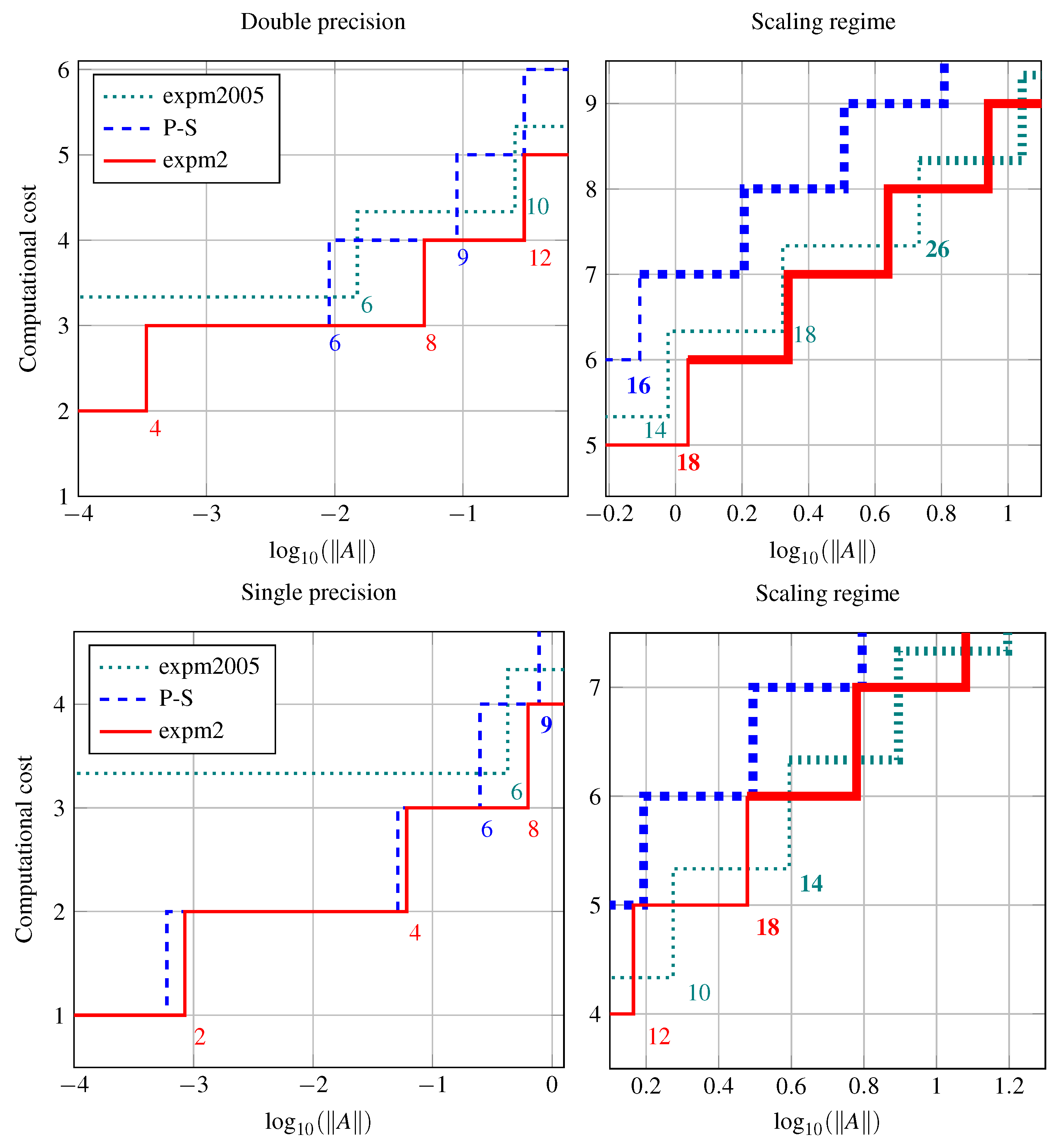
In Figure 1, we compare methods using the Taylor polynomial based on the Paterson-Stockmeyer (P-S) rule (with orders $2,4,6,9,16$) and on the new decompositions from Section 3, which we call expm2 (Algorithm 1, with orders $1,2,4,8,12,18$).

For reference, we also include the Padé approximants from [10] (with orders 6, 10, 14, 18, 26). The procedure, which we call expm2005, is implemented as expm in Matlab Release R2013a. We plot $\parallel A\parallel$ versus the cost measured as the number of matrix products necessary to approximate $e^A$, both in double (top) and single precision (bottom). For small values of $\parallel A\parallel$, the new approach to compute the Taylor approximant shows the best performance, whereas for higher values it has similar performance as the Padé method.    

Algorithm 1: expm2

Input: square matrix A.   orders := $\{1,2,4,8,12\}$.   for k in orders:     if ${\parallel A\parallel }_1<{\theta }_k$: return $T_k(A)$.   Apply scaling: $s=\lceil ({log}_2{(\parallel A\parallel }_1/{\theta }_{18})\rceil$, $A_s=2^{-s}A$;   Compute exponential: $E=T_{18}(A_s)$;   Apply s squarings to E and return result.

The right panels shows the scaling regime. We conclude that expm2 is superior (by $1/3$ matrix products) for around $2/3$ of the matrix norms considered in the graph and inferior (by $1/3$) for the remaining third. The percentage of the norm range where expm2 is cheaper can be computed by determining the points where both methods transition into the scaling regime, for expm2 at order 18 from ${log}_{10}(\parallel A\parallel )>0.037$ and for expm2005 at order 26 for ${log}_{10}(\parallel A\parallel )>0.732$. The difference is approximately $1/3mod{log}_{10}(2)$. For single precision, approximately the same conclusion holds. The corresponding points are ${log}_{10}(\parallel A\parallel )>0.479$ for expm2 (order 18) and ${log}_{10}(\parallel A\parallel )>0.594$ for expm2005 (order 14).

In Figure 1, we have limited ourselves to values of ${log}_{10}\parallel A\parallel$ of the order of 1, since for larger matrix norms, all the procedures require scaling and squaring.

In Figure 2, we compare expm2005 with our method expm2 for a range of test matrices. The color coding indicates the set to which the test matrix belongs: we have used nine matrices of type (17) where $b=1,10,\dots ,{10}^8$ (green); 46 different special matrices from the Matlab matrix gallery, as has been done in [10], sampled at different norms (blue); and randomly generated matrices.

Remark 5.

In all experiments, we used the same procedure to generate test matrices; the only difference is the dimensions of the matrices. The random number generator was seeded with 0 for reproducibility. We created 400 triangular matrices with elements from a uniform distribution $(0,1)$, 400 matrices taken from a standard normal distribution, 500 matrices from $(0,1)$ and another 500 matrices from $(-0.5,0.5)$. These matrices where rescaled by random numbers to yield norms in the interval $({10}^{-4},{10}^{4.1})$.Matlabfunctions to reproduce the results and generate the figures are available online [27].

Notice that the same experiment repeated with matrices of larger dimensions (up to $60\times 60$) or from a larger matrix test set shows virtually identical results.

For each matrix, we computed the exponential condition number [14]

$${\kappa }_{exp}(A):=\underset{ϵ\to 0}{lim}\underset{\parallel E\parallel \le ϵ\parallel A\parallel }{sup}\frac{\parallel e^{A+E}-e^A\parallel }{ϵ\parallel e^A\parallel },$$

and the reference solution $e^A$ was obtained using Mathematica with 100 digits of precision. From the top left panel, we see that both methods have relative errors $\parallel t_n-e^A\parallel /\parallel e^A\parallel$ close to machine accuracy for a wide range of matrices. We appreciate that for some special matrices, both methods have the potential to reach errors below machine accuracy. The same holds for slightly larger errors: for some matrices, especially large ones, both methods produce relative errors above machine accuracy. The top right panel confirms that due to smaller $\theta$ values of the Taylor polynomials, more scalings are needed for expm2 due to the smaller $\theta$ values from Table 1 compared with Table 2—the crosses are generally below the squares. The bottom left panel indicates that the new method expm2 is cheaper for a wide range of matrices as expected from Figure 1. The bottom right panel illustrates that the relative errors of the two methods lie within a range of two digits of each other. For the relative errors, we have taken the maximum between the obtained value and the machine accuracy in order to avoid misleading large differences at insignificant digits that can be appreciated in the top left panel.

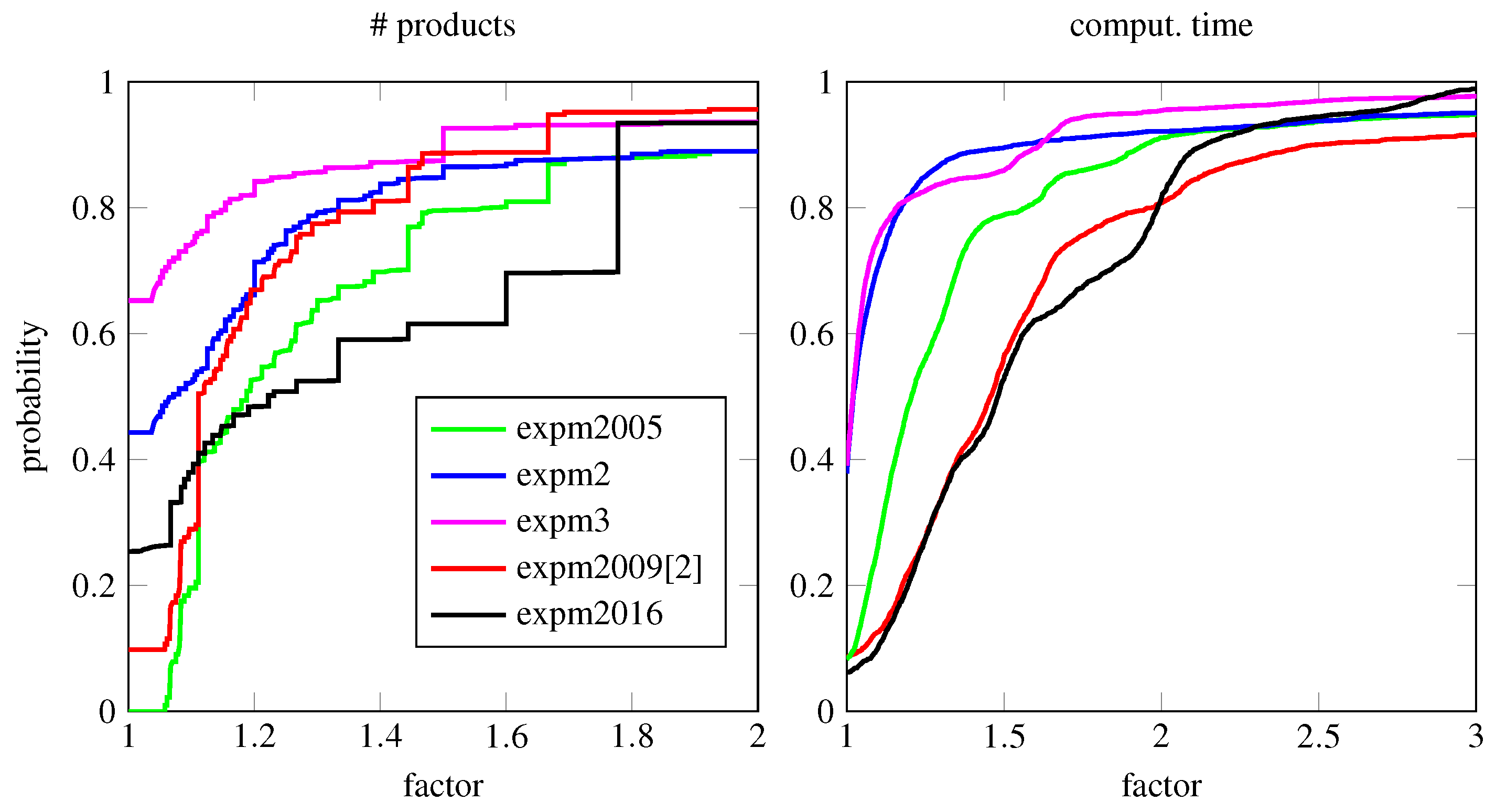
In Figure 3 (top row), we provide performance profiles for a larger test set comparing the methods expm2 and expm2005. Specifically, we have used 2500 matrices of dimensions $\le 64\times 64$ sampled as before (cf. Figure 2) from the Matlab matrix gallery, special matrices that are prone to overscaling, nilpotent matrices and random matrices. They have been scaled to cover a wide range of condition numbers. The bottom row anticipates the results from the methods expm3 and expm2009 [14] described below which incorporate norm estimators to avoid overscaling. From these plots, we can observe a clear improvement over the reference methods in terms of computational cost with only a minor impact on accuracy.

6. Refinement of Error Bounds to Avoid Overscaling

It has been noticed, in particular in [14,28,29], that the scaling and squaring technique based on the Padé approximant suffers from a phenomenon called overscaling: in some cases a value of s much larger than necessary is chosen, with the result of a loss of accuracy in floating point arithmetic. This feature is well illustrated by the following simple matrix proposed in [14]:

$$A=\left(\begin{array}{cc}1& b\\ 0& -1\end{array}\right),\mathrm{so} \mathrm{that}{e}^A=\left(\begin{array}{cc}e& \frac{b}{2}(e-e^{-1})\\ 0& e^{-1}\end{array}\right).$$

(17)

For $\left|b\right|\gg 1$, we have $\parallel A\parallel \approx \parallel e^A\parallel \ll e^{\parallel A\parallel }$ and the error bound previously considered in Section 1; namely,

$$\parallel h_{\ell }(A)\parallel \le {\tilde{h}}_{\ell }(\parallel A\parallel ),$$

leads to an unnecessarily large value of the scaling parameter s: the algorithm chooses a large value of s in order to verify the condition $\parallel 2^{-s}A\parallel <{\theta }_{\ell }$.

Needless to say, exactly the same considerations apply if we use instead a Taylor polynomial as the underlying approximation in the scaling and squaring algorithm.

This phenomenon can be alleviated by applying the strategy proposed in [14]. The idea consists of using the backward error analysis that underlies the algorithm in terms of the sequence $\{\parallel A^k{\parallel }^{1/k}\}$ instead of $\parallel A\parallel$, the reasoning being that for certain classes of matrices (in particular, for matrices of type (17)), $\parallel A^k{\parallel }^{1/k}$, $k>1$ is in fact much smaller than $\parallel A\parallel$.

If $\rho (A)$ denotes the spectral radius of A, one has in general

$$\rho (A)\le \parallel A^k{\parallel }^{1/k}\le \parallel A\parallel ,k=1,2,3,\dots ,$$

and moreover [14]

$$\parallel h_{\ell }(A)\parallel \le {\tilde{h}}_{\ell }(\parallel A^t{\parallel }^{1/t}),$$

where $\parallel A^t{\parallel }^{1/t}=max\{\parallel A^k{\parallel }^{1/k}:k\ge \ell and{c}_{\ell }\ne 0\}$. Since the value of t is not easy to determine, the following results are more useful in practice.

Lemma 1

([14]). For any $k\ge 1$ such that $k=p{m}_1+q{m}_2$ with $p,q\in \mathbb{N}$ and $m_1,m_2\in \mathbb{N}\cup \left\{0\right\}$,

$$\parallel A^k{\parallel }^{1/k}\le max\left(\parallel A^p{\parallel }^{1/p},{\parallel A^q\parallel }^{1/q}\right).$$

Theorem 1

([14]). Assuming that $\rho (A)<\omega$ and $p\in \mathbb{N}$, then

(a)

$\parallel h_{\ell }(A)\parallel \le {\tilde{h}}_{\ell }({\delta }_{p,p+1})$ if $\ell \ge p(p-1)$, with

$${\delta }_{p,p+1}\equiv max\left(\parallel A^p{\parallel }^{1/p},{\parallel A^{p+1}\parallel }^{1/(p+1)}\right);$$

(b)

$\parallel h_{\ell }(A)\parallel \le {\tilde{h}}_{\ell }({\delta }_{2p,2p+2})$ if $\ell \ge 2p(p-1)$ and $h_{\ell }$ is even, with

$${\delta }_{2p,2p+2}\equiv max\left(\parallel A^{2p}{\parallel }^{1/(2p)},{\parallel A^{2p+2}\parallel }^{1/(2p+2)}\right).$$

Denoting $d_k={\parallel A^k\parallel }^{1/k}$, ${\delta }_{i,j}=max(d_i,d_j)$, and applying Theorem 1 to the analysis of Section 1 allows one to replace the previous condition $\parallel 2^{-s}A\parallel <{\theta }_n$ by

$$2^{-s}min({\delta }_{p,p+1}:p(p-1)\le \ell )<{\theta }_{\ell },$$

or, if $h_{\ell }$ is an even function, as is the case with Padé approximants,

$$2^{-s}min({\delta }_{2p,2p+2}:2p(p-1)\le \ell )<{\theta }_{\ell }.$$

The algorithm proposed in [14], which is implemented from Matlab R2016a onward, incorporates the estimates from Theorem 1 (b) into the expm2005 (Padé) method; specifically, it computes $d_{4,6},d_{6,8}$ and $d_{8,10}$.

This process requires computing $\parallel A^r\parallel$ for some values of r for which $A^r$ have not been previously evaluated in the algorithm. In these cases, one may use the fast block 1-norm estimation algorithm of Higham and Tisseur [30] to get norm estimates correct within a factor 3 for $N\times N$ matrices. In this section, we consider the cost of these estimations to be scaling with $\mathcal{O}(N^2)$, and therefore neglect their contribution to the computational effort.

In order to reduce overscaling for the proposed algorithm expm2, we can only apply part (a) of Theorem 1 since the error expansion $h_{\ell }$ for the Taylor method is not an even function. It is not difficult to see, however, that the choices (a) and (b) in Theorem 1 are not the only options, and that other alternatives might provide even sharper bounds. We have to find pairs $(p_i,q_i)$ such that any $k\ge m$ can be written as $k=m_{1,i}{p}_i+m_{2,i}{q}_i$ for $m_{1,i},m_{2,i}\in \mathbb{N}\cup \left\{0\right\}$. Then, for Taylor polynomials of degree n we have the following possible choices, where obviously every pair also serves to decompose higher degrees:

$n=2$:

we have the pair $(2,3)$.

$n=4$:

we have, additionally, the pair $(2,5)$.

$n=8$:

the following pairs are also valid: $(2,7),(2,9),(3,4),(3,5)$.

$n=12$:

additionally, we obtain $(2,11),(2,13),(3,7),(4,5)$.

$n=18$:

additionally, $(2,15),(2,17),(2,19),(3,8),(3,10),(4,7)$.

To achieve a good compromise between extra computational cost from the norm estimations and reduction of overscaling we propose the following adjustments to our algorithm (see Algorithm 2).

Algorithm 2: expm3

Same as Algorithm 1 (expm2) for $\parallel A\parallel \le {\theta }_{18}$. For larger norms, degree 18 is selected, which requires the computation of these powers $A^2,A^3,A^6$. Now, calculate the roots of the norms of these products, $d_2,d_3,d_6$. Set $\eta =max(d_2,d_3)$. Heuristically, we say that there is a large decay in the norms of powers when $$min\left(\frac{d_2}{d_1},\frac{d_3}{d_1},\frac{d_6}{d_1}\right)\le \frac{1}{2^4}.$$ (18) This means that we can save at least four squarings using the right estimate. (To be precise, we need $min(d_3/d_2,d_9/d_2)<1/2^k$ to reduce the required squarings by k. In practice, however, the available fractions in (18) are sufficient to estimate the behavior at high powers.) If this is the case, then, we also estimate $d_9$ and update $\eta =min(\eta ,max(d_2,d_9))$. Finally, the number of scalings is given by $s=\lceil {log}_2(\eta /{\theta }_{18})\rceil$ and the order 18 decomposition is applied.

Remark 6.

For small matrix dimensions, it can be more efficient to explicitly compute matrix powers instead of using a sophisticated norm estimation algorithm. This is implemented inMatlabfor dimensions smaller than $150\times 150$. We point out that the additional products that are computed in this case can be used to increase the order of the Taylor methods following the procedures described in this work. The new problem formulation is then: given a set of matrix powers, which is the largest degree (Taylor) polynomial which can be computed at a given number of extra matrix products?

Algorithm expm3 is compared next with the refined method expm2009 [14], which is based on Theorem 1 (b) for the Padé approximants and additionally implements further estimates to refine the scaling parameter. The experimental setup is identical to the one of Figure 2. Recall that the computational cost of matrix norm estimates is not taken into account for either algorithm. The results are shown in Figure 4. The relative errors of the two methods are very similar. From the lower left panel, a clear cost advantage over the algorithm based on Padé approximants is apparent.

Finally, we have made a more extensive comparison of a variety of implementations tabulated in

Table 4. Algorithms used for Figure 5 grouped as: simple algorithms without norm estimates of type $d_k$ incorporated (expm2005, expm2); sophisticated algorithms to avoid overscaling (expm2009 [14], expm3); and an optimized official implementation from Matlab (expm2016), which contains several additional tweaks and modifications for expm2009 [14].

expm2005	Padé algorithm [10] as expm in Matlab Release R2013a.
expm2	Our Algorithm 1 using the decomposition of this work.
expm3	Our Algorithm 2 modified to avoid overscaling.
expm2009 [14]	Algorithm 3.2 from [14], based on Padé approximants and norm estimations through Theorem 1.
expm2016	Padé algorithm from [14] as expm in Matlab Release R2016a. This implementation contains special tweaks for small matrices, symmetric matrices Schur-decompositions and block structures.

. The performance profiles of the stated methods on a larger test set of special and random matrices predominantly of dimension $n\times n⪅1024\times 1024$ are displayed in Figure 5. Since the computation of the exact solution for this large test set was too costly, we only illustrated the performance plots for the number of required matrix products and the corresponding run times. The gain in computational speed is evident but less pronounced for some matrices because of the overhead from the norm estimations, which scale with $\mathcal{O}(n^2)$. For example, we can deduce that for $50\%$ of the test matrices, the Padé methods require at least 50% more computational time.

A highly relevant application of the matrix exponential is the (numerical) solution of matrix differential equations. Numerical methods such as exponential integrators, Magnus expansions or splitting methods typically force small matrix norms due to the small time-step inherent to the methods. In this case, the proposed algorithm expm2 should be highly advantageous.

7. Concluding Remarks

We have presented a new way to construct the Taylor polynomial, approximating the matrix exponential function up to degree 18, requiring less products than the Paterson-Stockmeyer technique. This reduction of matrix products is due to a particular factorization of the polynomial in terms of polynomials of lower degrees, where the coefficients of the factorization satisfy a system of algebraic equations. The algorithm requires $2,3,4$ and 5 matrix-matrix products to reach accuracy up to order $4,8,12$ and 18, respectively, showing similar cost to 1–2.5 commutators.

In combination with scaling and squaring, this yields a procedure to compute the matrix exponential up to the desired accuracy at lower computational cost than the standard Padé method for a wide range of matrices. Based on estimates of the form $\parallel A^k{\parallel }^{1/k}$ and the use of scaling and squaring, we have presented a modification of our algorithm to reduce overscaling that is still more efficient than state-of-the-art implementations with a slightly lower accuracy for some matrices but higher accuracy for others. The loss in accuracy can be attributed to possible overscalings due to a reduced number of norm estimations compared with Padé methods.

In practice, the maximal degree considered for the Taylor polynomial is 18 and the reduction in the number of matrix products required is due to a particular factorization of the polynomial in terms of polynomials of lower degrees whose coefficients satisfy an algebraic system of nonlinear equations.

The overall algorithm has been implemented as two different Matlab codes, available at [27]. The function expm2 corresponds to the simplest implementation based on the previous factorizations of the Taylor polynomials, whereas expm3 incorporates additional tools to deal with overscaling. Both are designed to be used in all circumstances where the standard Matlab function expm is called, and should provide equivalent results but requiring less computation time.

Although the technique developed here, combined with scaling and squaring, can be applied in principle to any matrix, it is clear that, in some cases, one can take advantage of the very particular structure of the matrix A, and then design especially tailored (and very often more efficient) methods for such problems [2,31,32]. For example, if one can find an additive decomposition $A=B+C$ such that $\parallel C\parallel$ is small and B is easy to exponentiate, i.e., $e^B$ is sparse and exactly solvable (or can be accurately and cheaply approximated numerically), and C is a dense matrix, then more efficient methods can be found in [12,33]. Exponentials of upper or lower triangular matrices A have been treated in [14], where it is shown that it is advantageous to exploit the fact that the diagonal elements of the exponential are exactly known. It is then, more efficient to replace the diagonal elements obtained numerically by the exact solution before squaring the matrix. This technique can also be extended to the first super or sub-diagonal elements. We plan to adapt this technique to other special classes of matrices appearing in physics, and in particular to compute in an efficient way the exponential of skew-Hermitian matrices, of great relevance in the context of quantum physics and chemistry problems.

For the convenience of the reader, we provide in [27], in addition to the Matlab implementations of the proposed schemes, the codes generating all the experiments and results reported here.

References

- Celledoni, E.; Marthinsen, H.; Owren, B. An introduction to Lie group integrators: Basics, new developments and applications. J. Comput. Phys. 2014, 257 Pt B, 1040–1061. [Google Scholar] [CrossRef] [Green Version]
- Iserles, A.; Munthe-Kaas, H.Z.; Nørsett, S.P.; Zanna, A. Lie group methods. Acta Numer. 2000, 9, 215–365. [Google Scholar] [CrossRef] [Green Version]
- Blanes, S.; Casas, F. A Concise Introduction to Geometric Numerical Integration; CRC Press: Boca Raton, FL, USA, 2016. [Google Scholar]
- Hairer, E.; Lubich, C.; Wanner, G. Geometric Numerical Integration. Structure-Preserving Algorithms for Ordinary Differential Equations, 2nd ed.; Springer: Berlin, Germany, 2006. [Google Scholar]
- Blanes, S.; Casas, F.; Oteo, J.A.; Ros, J. The Magnus expansion and some of its applications. Phys. Rep. 2009, 470, 151–238. [Google Scholar] [CrossRef] [Green Version]
- Casas, F.; Iserles, A. Explicit Magnus expansions for nonlinear equations. J. Phys. A Math. Gen. 2006, 39, 5445–5461. [Google Scholar] [CrossRef] [Green Version]
- Celledoni, E.; Marthinsen, A.; Owren, B. Commutator-free Lie group methods. Future Gener. Comput. Syst. 2003, 19, 341–352. [Google Scholar] [CrossRef] [Green Version]
- Crouch, P.E.; Grossman, R. Numerical integration of ordinary differential equations on manifolds. J. Nonlinear Sci. 1993, 3, 1–33. [Google Scholar] [CrossRef]
- Hochbruck, M.; Ostermann, A. Exponential integrators. Acta Numer. 2010, 19, 209–286. [Google Scholar] [CrossRef] [Green Version]
- Higham, N.J. The scaling and squaring method for the matrix exponential revisited. SIAM J. Matrix Anal. Appl. 2005, 26, 1179–1193. [Google Scholar] [CrossRef]
- Moler, C.B.; Van Loan, C.F. Nineteen dubious ways to compute the exponential of a matrix, twenty-five years later. SIAM Rev. 2003, 45, 3–49. [Google Scholar] [CrossRef]
- Najfeld, I.; Havel, T.F. Derivatives of the matrix exponential and their computation. Adv. Appl. Math. 1995, 16, 321–375. [Google Scholar] [CrossRef] [Green Version]
- Sidje, R.B. Expokit: A software package for computing matrix exponentials. ACM Trans. Math. Softw. 1998, 24, 130–156. [Google Scholar] [CrossRef]
- Al-Mohy, A.H.; Higham, N.J. A new scaling and squaring algorithm for the matrix exponential. SIAM J. Matrix Anal. Appl. 2009, 31, 970–989. [Google Scholar] [CrossRef] [Green Version]
- Bader, P.; Blanes, S.; Casas, F. An improved algorithm to compute the exponential of a matrix. arXiv 2017, arXiv:1710.10989. [Google Scholar]
- Higham, N.J.; Al-Mohy, A.H. Computing matrix functions. Acta Numer. 2010, 19, 159–208. [Google Scholar] [CrossRef] [Green Version]
- Baker, G.A., Jr.; Graves-Morris, P. Padé Approximants, 2nd ed.; Cambridge University Press: Cambridge, UK, 1996. [Google Scholar]
- Paterson, M.S.; Stockmeyer, L.J. On the number of nonscalar multiplications necessary to evaluate polynomials. SIAM J. Comput. 1973, 2, 60–66. [Google Scholar] [CrossRef] [Green Version]
- Higham, N.J. Functions of Matrices: Theory and Computation; Society for Industrial and Applied Mathematics: Philadelphia, PA, USA, 2008. [Google Scholar]
- Ruiz, P.; Sastre, J.; Ibáñez, J.; Defez, E. High perfomance computing of the matrix exponential. J. Comput. Appl. Math. 2016, 291, 370–379. [Google Scholar] [CrossRef]
- Sastre, J.; Ibáñez, J.; Ruiz, P.; Defez, E. New scaling-squaring Taylor algorithms for computing the matrix exponential. SIAM J. Sci. Comput. 2015, 37, A439–A455. [Google Scholar] [CrossRef]
- Sastre, J. Efficient evaluation of matrix polynomials. Linear Algebra Its Appl. 2018, 539, 229–250. [Google Scholar] [CrossRef]
- Westreich, D. Evaluating the matrix polynomial I + A + ⋯ + AN−1. IEEE Trans. Circuits Sys. 1989, 36, 162–164. [Google Scholar] [CrossRef]
- Lei, L.; Nakamura, T. A fast algorithm for evaluating the matrix polynomial I + A + ⋯ + AN−1. IEEE Trans. Circuits Sys. I Fundam. Theory Appl. 1992, 39, 299–300. [Google Scholar] [CrossRef]
- Higham, N.J. Accuracy and Stability of Numerical Algorithms; Society for Industrial and Applied Mathematics: Philadelphia, PA, USA, 1996. [Google Scholar]
- Arioli, M.; Codenotti, B.; Fassino, C. The Padé method for computing the matrix exponential. Linear Algebra Its Appl. 1996, 240, 111–130. [Google Scholar] [CrossRef] [Green Version]
- Bader, P.; Blanes, S.; Casas, F. An Efficient Alternative to the Function Expm of Matlab for the Computation of the Exponential of a Matrix. Available online: http://www.gicas.uji.es/Research/MatrixExp.html (accessed on 1 November 2019).
- Kenney, C.S.; Laub, A.J. A Schur-Fréchet algorithm for computing the logarithm and the exponential of a matrix. SIAM J. Matrix. Anal. Appl. 1998, 19, 640–663. [Google Scholar] [CrossRef]
- Dieci, L.; Papini, A. Padé approximation for the exponential of a block triangular matrix. Linear Algebra Its Appl. 2000, 308, 183–202. [Google Scholar] [CrossRef] [Green Version]
- Higham, N.J.; Tisseur, F. A block algorithm for matrix 1-norm estimation, with an application to 1-norm pseudospectra. SIAM J. Matrix Anal. Appl. 2000, 21, 1185–1201. [Google Scholar] [CrossRef]
- Celledoni, E.; Iserles, A. Approximating the exponential from a Lie algebra to a Lie group. Math. Comput. 2000, 69, 1457–1480. [Google Scholar] [CrossRef] [Green Version]
- Celledoni, E.; Iserles, A. Methods for the approximation of the matrix exponential in a Lie-algebraic setting. IMA J. Numer. Anal. 2001, 21, 463–488. [Google Scholar] [CrossRef] [Green Version]
- Bader, P.; Blanes, S.; Seydaoğlu, M. The scaling, splitting and squaring method for the exponential of perturbed matrices. SIAM J. Matrix Anal. Appl. 2015, 36, 594–614. [Google Scholar] [CrossRef] [Green Version]
Figure 1.
Optimal orders and their respective costs versus the norm of the matrix exponent. The numbers indicate the order of the approximants. Thick lines (right panels) show the cost when scaling and squaring is used and the corresponding orders are highlighted in bold-face.
Figure 2.
Comparison of expm2 and expm2005 for matrices of dimensions . The color coding corresponds to different test matrices: special matrices (17) (green), Matlab matrix gallery (blue), random matrices (red). Top left panel: The logarithmic relative errors of the two methods show similar values around machine accuracy (solid horizontal line). Top right panel: Number of squarings needed for each matrix. Bottom left: The relative cost of the method, counting matrix multiplications and inversions only. Bottom right: The difference of accurate digits is shown.
Figure 3.
Performance profiles to compare expm2 and expm2005, and expm3 and expm2009 [14] for matrices of dimensions . The left panels show the percentage of matrices that have a relative logarithmic error smaller than the abscissa. In the center panel, we see the percentage of matrices that can be computed using -times the number of products of the cheapest method for each problem. The right panel is a repetition of this experiment but shows the computation times (averaged over 10 runs) instead of the number of products.
Figure 4.
Comparison of algorithms expm3 and expm2009 [14] for matrices of dimension . Cf. Figure 2.
Figure 5.
Performance profiles for matrices of dimensions . We have used 2500 matrices from the Matlab matrix gallery, special matrices that are prone to overscaling, nilpotent matrices and random matrices, as indicated in Remark 5.