Geometric Numerical Integration in Ecological Modelling

Abstract

A major neglected weakness of many ecological models is the numerical method used to solve the governing systems of differential equations. Indeed, the discrete dynamics described by numerical integrators can provide spurious solution of the corresponding continuous model. The approach represented by the geometric numerical integration, by preserving qualitative properties of the solution, leads to improved numerical behaviour expecially in the long-time integration. Positivity of the phase space, Poisson structure of the flows, conservation of invariants that characterize the continuous ecological models are some of the qualitative characteristics well reproduced by geometric numerical integrators. In this paper we review the benefits induced by the use of geometric numerical integrators for some ecological differential models.

1. Introduction

Ecological modelling based on non linear differential systems of equations can be divided into two main categories [1]. Predictive modelling aims to reproduce, based on the knowledge provided by historical time series, the real observed phenomena and to predict their state in the future. Due to the large amount of uncertainty contained in ecological data, however, the approach of conceptual modelling is an effective alternative aimed to understand the main features of the ecological dynamics by making scenario analysis [2]. In both approaches, the mathematical model is based on governing laws described by non linear differential systems of equations. Their correct solution requires robust and accurate numerical algorithms; nevertheless, numerical schemes for ecological models have received little attention in the literature as most descriptions of models outline the governing equations but do not discuss their numerical solution. Indeed, it seems reasonable to assume that, within a predictive approach, numerical errors are always overwhelmed by uncertainties in the data and governing equations and to pay attention to numerical robustness is, therefore, unwarranted. On the other side, for conceptual modelling, first-order explicit numerical procedures are generally used in the belief that they are sufficient to infer potential future scenarios.

However, in literature, a rigorous numerical analysis is a recognized need due to the often neglected fact that the dynamics of the numerical flow can differ significantly from that of the original differential system:

• ‘An inadequate choice of a numerical method may have a detrimental effect on the study by making simulations costly and even producing wrong results’ [1];
• ‘Erroneous or misleading conclusions of model analysis and prediction arising from numerical artifacts in hydrological models are intolerable’ [3];
• ‘The literature abounds with examples of spurious behavior of numerical solutions, e.g., spurious fixed points, numerical ’chaos’, and spurious periodicity’ [4].

In the last decades, the theory of numerical methods allowed excellent general-purpose codes, mainly based on Runge Kutta methods or linear multistep methods. The born of the geometric numerical integration operated in the literature a shift of view-point: a numerical method is viewed as a discrete dynamical system which approximates the flow of the differential equation while preserving some of its specific properties. These are crucial for a qualitatively correct simulation of the dynamics and always improve long-time numerical behaviour [5].

In ecological modelling, the approximated solutions should be able to reproduce the main physical qualitative characteristics of the observed quantities (e.g., positive concentrations, mass/energy conservation) in order to make accurate previsions or outline realistic scenarios. For this reason, geometric numerical integration plays a crucial role in the analysis of ecosystem models described by systems of differential equations. The principal flow structures that arise in ecological modelling and that have to be preserved are Poisson maps. By means of the Darboux-Lie theorem, it is possible to find a transformation such that in the novel coordinates, a Poisson problem assumes a canonical Hamiltonian form. Then, symplectic methods, as for example collocation methods [6], are convenient for the structure preserving long-time integration. In this regard, as the order of the error of the collocation method is basically the same as of the underlying quadrature rule, one can exploit the Gaussian splines rules [7,8,9], for numerical integration to keep the same order of error, while requiring fewer quadrature points [5]. Instead of trasforming Poisson maps in Hamiltonian maps, in this review we will describe discrete dynamical systems that directly preserve the Poisson structure. They will correspond to Poisson numerical integrators of Poisson ecological systems. We will show their properties and the gain in performance with respect to classical procedures.

Other aspects that, in the nonlinear context, are alternative to the preservation of the structure of the flow, but not less important, are the phase-space preservation [10] and the conservation of invariants (see, for example, [11,12]). Indeed, since in computational ecology all involved quantities (i.e., densities, masses or concentrations) should be nonnegative, is of outmost importance to preserve the positive phase-space of the dynamics in order to produce physically valid numerical approximations. Moreover, approximations that preserve linear invariants are able to provide more accurate description of biogeochemical processes in ecosystem models [13].

In this paper, we will describe the application and the results of the analysis of geometric numerical integration in the framework of ecological modeling. For both predictive and conceptual real world modelling, the use of geometric numerical integration was indeed the favourite tool for making accurate qualitative scenario analysis and saving computational time [14,15]. Limiting to first-order procedures, we will illustrate the most suitable geometric numerical integrators for some ecosystem dynamics models. For optimal control problems that model management policies, we will describe the advantage of the symplectic Runge-Kutta pairs in order to get efficient methods easy to be implemented within any numerical software [16]. Finally, as future perspective, we will present some examples of ecological models featured by both Poisson and biochemical structure [17] and we will discuss about some open questions related to their numerical approximation.

2. Poisson Integrators for Poisson Systems in Ecology

Ecosystem population dynamics, including organism such as algae, invertebrates, fish, large herbivores and carnivores, are characterized by the interaction between predator and prey populations that controls and drives changes in populations over time. When resources are limited, individuals compete for access to resources, and populations decline. To survive and reproduce, they must obtain sufficient food while simultaneously avoiding becoming food for a predator. To address the trade-off between food intake and predator avoidance, ecologists have turned to mathematical models to better understand foraging behavior and predator-prey dynamics. Lotka-Volterra models provide the main tool to help population ecologists understand the factors that influence population dynamics. Although the models greatly simplify actual conditions, they demonstrate that under certain circumstances, predator and prey populations can oscillate over time in a manner similar to that observed in the real-word.

The Lotka-Volterra model falls in the more general class of ecological models called M-systems [18] for which population dynamics is described by Poisson systems analogous to the Hamiltonian formulation of classical mechanics. Other important examples of ecological differential models featured by a Poisson structure can be found among multispecies Lotka-Volterra systems [19]. The classical example is the Rock-Paper–scissor model based on relationships that characterize communities without strict competitive hierarchies [20].

We will see that the geometric numerical integration of ecological models featured by a Poisson dynamics, performed by means of Poisson integrators [5], especially over long time horizons, improves the qualitative results and, consequently the analysis of ecosystems scenarios.

Before entering into the details, we recall that, given a vector-valued scalar function $H=H(y;t)$, called Hamiltonian function, a Poisson system is defined by the differential equation ${\displaystyle {\displaystyle \frac{dy}{dt}}=B\left(y\right)\nabla H,}$ where $B\left(y\right)$ is a matrix skew-symmetric operator and satisfies

$${\displaystyle \sum _{l=1}^n\left({\displaystyle \frac{\partial b_{ij}\left(y\right)}{\partial y_l}{b}_{lk}\left(y\right)+\frac{\partial b_{jk}\left(y\right)}{\partial y_l}{b}_{li}\left(y\right)+\frac{\partial b_{ki}\left(y\right)}{\partial y_l}{b}_{lj}\left(y\right)}\right)=0}$$

(1)

for all $i,j,k$ ( the Jacobi identity). The flow ${\phi }_t\left(y\right)$ of a Poisson-system is a Poisson map i.e., its Jacobian matrix ${\varphi }_t^{\prime }$ satisfies

$${\phi }_t^{\prime }\left(y\right)B\left(y\right){\phi }_t^{\prime }{\left(y\right)}^T=B\left({\phi }_t\left(y\right)\right).$$

If the skew-symmetric operator $B\left(y\right)$, which allows to define a Poisson bracket, is of constant rank $n-q=2r$, then there exist q functions $C_1\left(y\right),C_2\left(y\right),\cdots C_q\left(y\right)$ called Casimirs, which satisfy $\nabla C_i{\left(y\right)}^{T}B\left(y\right)=0.$ Consequently,

$$\{C_i,H\}\left\{y\right\}(=\nabla C_i{\left(y\right)}^{T}B\left(y\right)\nabla H\left(y\right))=0,$$

resulting Casimirs first integrals of Poisson system for all Hamiltonian function H.

In the next section, we provide two model examples representative of Poisson dynamics in ecology and we review the principal Poisson integrators developed in the recent literature for their numerical approximation. Moreover, we will illustrate the rock-scissor-paper model and the Hirota’s algorithm for its numerical approximation.

2.1. Dynamical M-System

There exists a wide class of systems in ecology, that are called M-systems, for which population dynamics can be described by a phase-space theory analogous to the Hamiltonian formulation of classical mechanics [18]. An M-system is a dynamical system defined by a given resource function M$(u,v;t)$ and equation of motions given by

$${\displaystyle \dot{u}=-uv\frac{\partial M}{\partial v},\dot{v}=uv\frac{\partial M}{\partial u}.}$$

By setting $y=(u,v)$, it is easy to see that M-systems are special cases of Poisson systems ${\displaystyle {\displaystyle \frac{dy}{dt}}=B\left(y\right)\nabla M}$ with Hamiltonian function M$(y;t)$ and skew-symmetric matrix operator

$$B\left(y\right)=\left(\begin{array}{cc}0& -uv\\ uv& 0\end{array}\right)$$

(2)

which satisfies the Jacobi identity (1). By considering the change of variables: $\tilde{u}=ln(u/\sigma ),\tilde{v}=ln(v/\xi )$ where $\sigma ,\xi >0$, the class of M-system on ${\mathbb{R}}_{+}^2$ has an associated Hamiltonian system

$${\displaystyle \dot{\tilde{u}}=-\frac{\partial H}{\partial \tilde{v}},\dot{\tilde{v}}=\frac{\partial H}{\partial \tilde{u}}}$$

where $H(\tilde{u},\tilde{v};t)=M(u\left(\tilde{u}\right),v\left(\tilde{v}\right);t)$ is the Hamiltonian function. Notice that, the relations comprise the positive Poisson phase plane ${\mathbb{R}}_{+}^2$ into the Hamiltonian phase plane ${\mathbb{R}}^2$; conversely, the inverted relations comprise the Hamilton phase space ${\mathbb{R}}^2$ into the positive Poisson phase plane ${\mathbb{R}}_{+}^2$.

The first example of a positive M-system is given by the Lotka-Volterra dynamics that, in adimensional variables is written as

$$\dot{u}=(a-v)u,\dot{v}=(u-b)v.$$

In this case, the resource function M$(u,v)$ is given by $M(u,v)=-alnv+v-blnu+u$ (see also [5], Sec VII.2.2). It represents an example of separable M-system as the resource function is separable in two parts, one depending on u and the other on v i.e., $M(u,v)=K\left(u\right)+L\left(v\right)$ with $K\left(u\right)=u-blnu$ and $L\left(v\right)=v-alnv$.

The second example of positive M-system considers a two-species system described by the equations

$${\displaystyle \dot{u}=u(\gamma +\mu vln\frac{u}{u_s}),\dot{v}=v(k-\mu v).}$$

(3)

where the second equation defines the logistic evolution, $\gamma$ and k are the growing rate for the population u and v respectively ; $\mu v$ represents the density dependent mortality rate, and $u_s$ is a saturation constant. The corresponding M-function is defined by

$${\displaystyle M=-\gamma lnv+klnu-\mu vln\frac{u}{u_s}.}$$

Notice that, in this case, M is not separable in two parts each depending on only one variable.

2.2. Poisson Integrators for M-Systems

Given a dynamical M-system, a numerical one-step method $y_{n+1}={\Phi }_{\Delta t}\left(y_n\right)$ is called Poisson integrator for a M-system if it is a Poisson map whenever applied to the M-system i.e., if the Jacobian ${\Phi }_{\Delta t}{\left(y_n\right)}^{\prime }$ satisfies

$${\Phi }_{\Delta t}{\left(y_n\right)}^{\prime }B\left(y_n\right){\Phi }_{\Delta t}{\left(y_n\right)}^{\prime T}=B\left({\Phi }_{\Delta t}\left(y_n\right)\right).$$

where B (of full rank) is defined in Equation (2).

The Symplectic Euler scheme

$${\displaystyle \frac{u^{n+1}-u^n}{\Delta t}=-u^{n+1}{v}^n\frac{\partial M}{\partial v}(u^{n+1},v^n),\frac{v^{n+1}-v^n}{\Delta t}=u^{n+1}{v}^n\frac{\partial M}{\partial u}(u^{n+1},v^n)}$$

is a Poisson integrator for separable M-system. It is implicit, it is not a Poisson integrator for general non-separable M-system and, in general, starting from positive values, it does not provide positive solutions without constraining the stepsize. This constraint, for Lotka-Volterra dynamics results stronger than the condition required by the linear stability analysis [21].

The explicit variant of symplectic Euler [22]

$${\displaystyle \frac{u^{n+1}-u^n}{\Delta t}=-u^n{v}^n\frac{\partial M}{\partial v}(u^n,v^n),\frac{v^{n+1}-v^n}{\Delta t}=u^{n+1}{v}^n\frac{\partial M}{\partial u}(u^{n+1},v^n)}$$

is a Poisson integrator for a separable M-systems. As symplectic Euler is not a Poisson integrator for general non-separable M-systems and in general, starting from positive solution, it does not provide positive solutions. When applied to Lotka-Volterra dynamics, the condition for positivity for exponentially long-time intervals gained by means of backward error analysis, is stronger than conditions given by the linear stability analysis [21]. The main advantage is its explicit functional form.

A Poisson integrator, suitable for positive M-systems, is Poisson Euler [5]:

$$u^{n+1}=u^n{e}^{{\displaystyle -\Delta t{v}^n\frac{\partial M}{\partial v}(u^{n+1},v^n)}},v^{n+1}=v^n{e}^{{\displaystyle \Delta t{u}^{n+1}\frac{\partial M}{\partial u}(u^{n+1},v^n).}}$$

(4)

together with its adjoint. In the following, we recall the main properties proved in [23].

Theorem 1.

The first-order method (4) is a Poisson integrator for M-systems for any resource M-function such that ${\displaystyle 1+\Delta t{u}^{n+1}{v}^n\frac{{\partial }^{2}M}{\partial u\partial v}(u^{n+1},v^n)\ne 0}$. It provides positive solutions for all $\Delta t>0$ whenever $v_0,u_0$ are positive. In case of separable M-systems it is also explicit.

Theorem 2.

Provided that ${\displaystyle \Delta t<\frac{2}{\sqrt{ab}}}$, the numerical scheme (4), linearized around the equilibria, has the same stability properties of the Lotka-Volterra model i.e., it has a saddle point at the origin and a neutral center at the internal equilibrium ${\displaystyle (b,a).}$

Form the above properties, Poisson Euler provides positive solutions without constraints on the choice of the stepsize and has the same linear stability constraints of the Symplectic Euler method when applied to Lotka-Volterra dynamics. For separable M-systems it is explicit while it results implicit for non separable M-systems. This drawback is not overcome by the Explicit Variant of Poisson Euler scheme, given by

$$u^{n+1}=u^n{e}^{{\displaystyle -\Delta t{v}^n\frac{\partial M}{\partial v}(u^n,v^n)}},v^{n+1}=v^n{e}^{{\displaystyle \Delta t{u}^{n+1}\frac{\partial M}{\partial u}(u^{n+1},v^n),}}$$

as it results a discrete Poisson map only in case of separable M-system. To illustrate the performance of the methods, we approximate the solution of Equation (3) which represents a not separable M-system. In Figure 1 the gain in performance of the Poisson Euler schemes with respect to Symplectic Euler schemes is illustrated.

2.3. Positive Integrators for Generic Predator-Prey Dynamics

Consider a generic two-species predator-prey system

$$\dot{u}=f(u,v),\dot{v}=g(u,v).$$

The idea to perform the log transform, apply a symplectic Runge-Kutta scheme and then transform back by the exponential, allows to build numerical integrators able to provide positive approximations [23]. The first order variants of these schemes, that we continue to call Poisson Euler as it generalizes the Poisson Euler for M-dynamics, are given by:

$${\displaystyle {\Phi }_{\Delta t}^{\left[R\right]}:u^{n+1}=u^n{e}^{{\displaystyle \Delta t\frac{f(u^{n+1},v^n)}{u^{n+1}}}},v^{n+1}=v^n{e}^{{\displaystyle \Delta t\frac{g(u^{n+1},v^n)}{v^n}}}}$$

(5)

with its explicit variant

$${\displaystyle \Sigma \left({\Phi }_{\Delta t}^{\left[R\right]}\right):u^{n+1}=u^n{e}^{{\displaystyle \Delta t\frac{f(u^n,v^n)}{u^n}}},v^{n+1}=v^n{e}^{{\displaystyle \Delta t\frac{g(u^{n+1},v^n)}{v^n}}},}$$

(6)

its adjoint

$${\displaystyle {\Phi }_{\Delta t}^{\left[R\right]*}:v^{n+1}=v^n{e}^{{\displaystyle \Delta t\frac{g(u^n,v^{n+1})}{v^{n+1}}}},u^{n+1}=u^n{e}^{{\displaystyle \Delta t\frac{f(u^n,v^{n+1})}{u^n}}},}$$

(7)

and its explicit variant

$${\displaystyle \Sigma \left({\Phi }_{\Delta t}^{\left[R\right]*}\right):v^{n+1}=v^n{e}^{{\displaystyle \Delta t\frac{g(u^n,v^n)}{v^n}}},u^{n+1}=u^n{e}^{{\displaystyle \Delta t\frac{f(u^n,v^{n+1})}{u^n}}}.}$$

(8)

Notice that, when $f(u,v)=uF\left(v\right)$ then Poisson Euler method (5) results explicit; similarly, when $g(u,v)=vG\left(u\right)$ the adjoint method (7) results explicit too. In the sequel, the performance of these positive schemes will be illustrated when applied to the approximation of the reaction semiflow of a spatially explicit dynamics.

2.4. Comparison Among Integrators

In

Table 1. Comparison among first-order methods: properties (N = No, Y = Yes) and computational complexity (E = explicit, I = implicit, SI = semi-implicit, LSI = linearly semi-implicit, see Section 2.4 for further details). The symbol ∘ denotes the Hadamard (elementwise) product.

Methods	EE	IE	SE	EVSE	SE *	EVSE *	PE	EVPE	PE *	EVPE *
Unconditionally Positive
$\dot{\mathbf{u}}=\mathbf{f}(\mathbf{u},\mathbf{v})$	N	Y	N	N	N	Y	Y	Y	Y	Y
$\dot{\mathbf{v}}=\mathbf{g}(\mathbf{u},\mathbf{v})$
Poisson Structure
$\dot{u}=-uv{\displaystyle \frac{\partial M}{\partial u}}$	N	N	M sep. Y	M sep. Y	M sep. Y	M sep. Y	Y	M sep. Y	Y	M sep. Y
$\dot{v}=uv{\displaystyle \frac{\partial M}{\partial v}}$
Functional Form
$\dot{\mathbf{u}}=\mathbf{f}(\mathbf{u},\mathbf{v})$	E	I	SI	E	SI	E	SI	E	SI	E
$\dot{\mathbf{v}}=\mathbf{g}(\mathbf{u},\mathbf{v})$
$\dot{\mathbf{u}}=\mathbf{u}\circ \mathbf{F}\left(\mathbf{v}\right)$	E	I	LSI	E	SI	E	E	E	SI	E
$\dot{\mathbf{v}}=\mathbf{g}(\mathbf{u},\mathbf{v})$
$\dot{\mathbf{u}}=\mathbf{f}(\mathbf{u},\mathbf{v})$	E	I	SI	E	LSI	E	SI	E	E	E
$\dot{\mathbf{v}}=\mathbf{v}\circ \mathbf{G}\left(\mathbf{u}\right)$

we summarize the properties of the main first-order geometric numerical integrators here proposed and we compare their computational complexity with respect to classical explicit and implicit Euler schemes. To generalize the proposed approaches to $2N$ dimensional interactions with $N>1$, we refer to the solution of the ODE system

$$\dot{\mathbf{u}}=\mathbf{f}(\mathbf{u},\mathbf{v}),\dot{\mathbf{v}}=\mathbf{g}(\mathbf{u},\mathbf{v})$$

where $\mathbf{u},\mathbf{v},\mathbf{f},\mathbf{g}\in {\mathbb{R}}^N.$ We leave out the costs due to the evaluation of N-dimensional vector functions and we account only for the solution of systems of equations. We distinguish the methods according to their functional form:

• explicit (E); at each step only function evaluations are performed;
• implicit (I); at each step the method requires the solution of a $2N$-dimensional system of nonlinear equations;
• semi-implicit (SI) at each step the method requires the solution of an N-dimensional system of nonlinear equations;
• linearly semi-implicit (LSI); at each step the method requires the solution of an N-dimensional system of linear equations.

The method considered are listed below.

• Explicit Euler (EE)

  $${\displaystyle \frac{{\mathbf{u}}^{n+1}-{\mathbf{u}}^n}{\Delta t}=\mathbf{f}({\mathbf{u}}^n,{\mathbf{v}}^n),\frac{{\mathbf{v}}^{n+1}-{\mathbf{v}}^n}{\Delta t}=\mathbf{g}({\mathbf{u}}^n,{\mathbf{v}}^n);}$$
• Implicit Euler (IE)

  $${\displaystyle \frac{{\mathbf{u}}^{n+1}-{\mathbf{u}}^n}{\Delta t}=\mathbf{f}({\mathbf{u}}^{n+1},{\mathbf{v}}^{n+1}),\frac{{\mathbf{v}}^{n+1}-{\mathbf{v}}^n}{\Delta t}=\mathbf{g}({\mathbf{u}}^{n+1},{\mathbf{v}}^{n+1});}$$
• Symplectic Euler (SE)

  $${\displaystyle \frac{{\mathbf{u}}^{n+1}-{\mathbf{u}}^n}{\Delta t}=\mathbf{f}({\mathbf{u}}^{n+1},{\mathbf{v}}^n),\frac{{\mathbf{v}}^{n+1}-{\mathbf{v}}^n}{\Delta t}=\mathbf{g}({\mathbf{u}}^{n+1},{\mathbf{v}}^n);}$$
• Explicit Variant of Symplectic Euler (EVSE)

  $${\displaystyle \frac{{\mathbf{u}}^{n+1}-{\mathbf{u}}^n}{\Delta t}=\mathbf{f}({\mathbf{u}}^n,{\mathbf{v}}^n),\frac{{\mathbf{v}}^{n+1}-{\mathbf{v}}^n}{\Delta t}=\mathbf{g}({\mathbf{u}}^{n+1},{\mathbf{v}}^n);}$$
• Adjoint of Symplectic Euler (SE${}^{*}$)

  $${\displaystyle \frac{{\mathbf{u}}^{n+1}-{\mathbf{u}}^n}{\Delta t}=\mathbf{f}({\mathbf{u}}^n,{\mathbf{v}}^{n+1}),\frac{{\mathbf{v}}^{n+1}-{\mathbf{v}}^n}{\Delta t}=\mathbf{g}({\mathbf{u}}^n,{\mathbf{v}}^{n+1});}$$
• Explicit Variant of the adjoint of Symplectic Euler (EVSE${}^{*}$)

  $${\displaystyle \frac{{\mathbf{u}}^{n+1}-{\mathbf{u}}^n}{\Delta t}=\mathbf{f}({\mathbf{u}}^n,{\mathbf{v}}^{n+1}),\frac{{\mathbf{v}}^{n+1}-{\mathbf{v}}^n}{\Delta t}=\mathbf{g}({\mathbf{u}}^n,{\mathbf{v}}^n);}$$
• Poisson Euler (PE)

  $${\displaystyle u_i^{n+1}=u_i^n{e}^{{\displaystyle \Delta t\frac{f_i({\mathbf{u}}^{n+1},{\mathbf{v}}^n)}{u_i^{n+1}}}},v_i^{n+1}=v_i^n{e}^{{\displaystyle \Delta t\frac{g_i({\mathbf{u}}^{n+1},{\mathbf{v}}^n)}{v_i^n}}},i=1,\cdots ,N;}$$
• Explicit Variant of Poisson Euler (EVPE)

  $${\displaystyle u_i^{n+1}=u_i^n{e}^{{\displaystyle \Delta t\frac{f_i({\mathbf{u}}^n,{\mathbf{v}}^n)}{u_i^n}}},v_i^{n+1}=v_i^n{e}^{{\displaystyle \Delta t\frac{g_i({\mathbf{u}}^{n+1},{\mathbf{v}}^n)}{v_i^n}}},i=1,\cdots ,N;}$$
• Adjoint of Poisson Euler (PE${}^{*}$)

  $${\displaystyle u_i^{n+1}=u_i^n{e}^{{\displaystyle \Delta t\frac{f_i({\mathbf{u}}^n,{\mathbf{v}}^{n+1})}{u_i^n}}},v_i^{n+1}=v_i^n{e}^{{\displaystyle \Delta t\frac{g_i({\mathbf{u}}^n,{\mathbf{v}}^{n+1})}{v_i^{n+1}}}},i=1,\cdots ,N;}$$
• Explicit Variant of the adjoint of Poisson Euler (EVPE${}^{*}$)

  $${\displaystyle u_i^{n+1}=u_i^n{e}^{{\displaystyle \Delta t\frac{f_i({\mathbf{u}}^n,{\mathbf{v}}^{n+1})}{u_i^n}}},v_i^{n+1}=v_i^n{e}^{{\displaystyle \Delta t\frac{g_i({\mathbf{u}}^n,{\mathbf{v}}^n)}{v_i^n}}},i=1,\cdots ,N.}$$

2.5. Hirota’s Scheme for Rock-Paper-Scissors Model

The classic system, that involves a community of three competing species satisfying a relationship similar to the children’s game Rock-Paper-scissors, has been considered in [20] to study how local dispersal promotes biodiversity for non-transitive communities, that is, those without strict competitive hierarchies. Such relationships, where rock crushes scissors, scissors cuts paper, and paper covers rock have been demonstrated in several natural systems (see for example [24,25]). The dynamical model is described by a three species Lotka-Volterra system:

$${\displaystyle \dot{u}=u(z-v),\dot{z}=z(v-u),\dot{v}=v(u-z).}$$

By setting $y=(u,z,v)$, the three species model may be defined ad Poisson systems in two ways:

$${\displaystyle \frac{dy}{dt}}=B_1\nabla H_{2}or{\displaystyle \frac{dy}{dt}}=B_2\nabla H_1,$$

where

$$B_1\left(y\right)=\left(\begin{array}{ccc}0& -1& 1\\ 1& 0& -1\\ -1& 1& 0\end{array}\right),B_2\left(y\right)=\left(\begin{array}{ccc}0& uz& -uv\\ -uz& 0& zv\\ uv& -zv& 0\end{array}\right),$$

and $H_1=u+z+v,H_2=uzv.$ $H_1$ is the Casimir w.r.t. the Poisson bracket defined by $B_1$ and $H_2$ is the Casimir w.r.t. the Poisson bracket defined by $B_2$.

A numerical one-step method $y_{n+1}={\Phi }_{\Delta t}\left(y_n\right)$ is a Poisson integrator for the above three species Lotka-Volterra system if the Jacobian ${\Phi }_{\Delta t}{\left(y_n\right)}^{\prime }$ is a Poisson map w.r.t. $B_1$ which preserves the Casimir $H_1$ or is a Poisson map w.r.t. $B_2$ which preserves the Casimir $H_2$. Hirota’s algorithm given in [26] for the above three-species example, is described by the following iterative scheme [19] :

$${\displaystyle \frac{u^{n+1}-u^n}{\Delta t}=u^n{z}^n-u^{n+1}{v}^{n+1},\frac{z^{n+1}-z^n}{\Delta t}=z^n{v}^n-z^{n+1}{u}^{n+1},\frac{v^{n+1}-v^n}{\Delta t}=v^n{u}^n-v^{n+1}{z}^{n+1}.}$$

It results that it is a Poisson integrator for ${\displaystyle \frac{dy}{dt}}=B_2\nabla H_1$ i.e., it is a Poisson map w.r-t $B_2$ which preserves the Casimir $H_2$.

Another important geometric aspect of the Hirota’s algorithm is the preservation of positivity. Indeed, starting from positive values, it provides positive solutions without constraints on the choice of stepsize. This can be shown by writing the Hirota’s algorithm as:

$$\begin{array}{c}{\displaystyle u^{n+1}=\frac{u^n({\Delta t}^2{z}^n{v}^n+\Delta t{z}^n+1)}{{\Delta t}^2{v}^n{u}^n+\Delta t{v}^n+1},}\hfill \\ {\displaystyle z^{n+1}=\frac{z^n({\Delta t}^2{v}^n{u}^n+\Delta t{v}^n+1)}{{\Delta t}^2{u}^n{z}^n+\Delta t{u}^n+1},}\hfill \\ {\displaystyle v^{n+1}=\frac{v^n({\Delta t}^2{u}^n{z}^n+\Delta t{u}^n+1)}{{\Delta t}^2{z}^n{v}^n+\Delta t{z}^n+1}.}\hfill \end{array}$$

3. Poisson Integrators for Spatially Extended Ecosystem Dynamics

In the previous section, we have recalled that the predator-prey interactions of different species, are extremely important in some temporal ecological problems. Although the space has been neglected so far, to describe the onset of important phenomena in some ecosystems dynamics, the spatial factors should be included in the model.

3.1. Poisson Euler for Turing Patterns Occurrence in a Ratio-Dependent Phytoplankton-Zooplankton Model

When space is included in the models, the formation of spatial patterns constitutes a very active research area in ecosystem modelling, based on the pioneering work of Turing [27]. There is a huge literature on the subject; however, to show the benefits of using Poisson integrators for predicting the onset of Turing patterns here we will focus on the specific model described in [28]. It is a three-chain coupled map lattice model built for exploring the spatiotemporal complexity of a predator-prey system with migration and diffusion. Based on Turing instability analysis, the authors derive pattern formation conditions for the predator-prey system. Via numerical simulation, Turing patterns can be found with subtle self organized structures under diffusion-driven and migration-driven mechanisms. It is evident that, if the aim of numerical simulation is to establish the formation of patterns, it is crucial to have numerical flows which share the same qualitative characteristics of the theoretical ones.

The model is a ratio-dependent phytoplankton- zooplankton model in a two dimensional space $\Omega ={[0,L]}^2$. Periodic boundary conditions are set and dynamics is described by

$$\begin{array}{ccc}{\displaystyle \frac{\partial P}{\partial t}}\hfill & =& k_P{\nabla }^{2}P-W_g{\displaystyle \frac{\partial P}{\partial x}}+rP\left(1-{\displaystyle \frac{P}{k}}\right)-{\displaystyle \frac{kPZ}{Z+kP}}\hfill \\ {\displaystyle \frac{\partial Z}{\partial t}}\hfill & =& k_Z{\nabla }^{2}Z+{\displaystyle \frac{kPZ}{Z+kP}}-m_{z}Z.\hfill \end{array}$$

(9)

Linear stability analysis established that $(P_1,Z_1)=(k,0)$ is an unstable equilibrium of the local dynamics. Under the hypothesis that $m_z<1$ and $r+k(m_z-1)>0$, the equilibrium $(P_2,Z_2)=\left({\displaystyle \frac{k(r+k(m_z-1))}{r}},{\displaystyle \frac{k^2(1-m_z)(r+k(m_z-1)}{m_{z}r}}\right)$ is stable.

Given $P_{i,j}^{\left(n\right)}$, $Z_{i,j}^{\left(n\right)}$ representing prey and predator density in the $(i,j)$ spatial cell at the time $t_n=t_0+n\Delta t$, the discrete flow is split in advection–diffusion–reaction (ADR) semiflows:

• discrete advection semiflow: given ${\Gamma }_d{\Psi }_{i,j}^{\left(n\right)}:={\Psi }_{i-1,j}^{\left(n\right)}-{\Psi }_{i,j}^{\left(n\right)}$,

  $${\tilde{P}}_{i,j}^{\left(n\right)}=P_{i,j}^{\left(n\right)}+{\displaystyle \frac{\Delta t}{\Delta x}}{W}_g{\Gamma }_d{P}_{i,j}^{\left(n\right)},{\tilde{Z}}_{i,j}^{\left(n\right)}=Z_{i,j}^{\left(n\right)},$$
• discrete diffusive semiflow: given ${\Delta }_d{\Psi }_{i,j}^{\left(n\right)}:={\Psi }_{i+1,j}^{\left(n\right)}+{\Psi }_{i-1,j}^{\left(n\right)}+{\Psi }_{i,j+1}^{\left(n\right)}+{\Psi }_{i,j-1}^{\left(n\right)}-4{\Psi }_{i,j}^{\left(n\right)}$,

  $${\overline{P}}_{i,j}^{\left(n\right)}={\tilde{P}}_{i,j}^{\left(n\right)}+{\displaystyle \frac{\Delta t}{\Delta x^2}}{k}_P{\Delta }_d{\tilde{P}}_{i,j}^{\left(n\right)},{\overline{Z}}_{i,j}^{\left(n\right)}={\tilde{Z}}_{i,j}^{\left(n\right)}+{\displaystyle \frac{\Delta t}{\Delta x^2}}{k}_Z{\Delta }_d{\tilde{Z}}_{i,j}^{\left(n\right)},$$
• discrete reaction semiflow: advances in time with the explicit variant of (the adjoint of) Poisson-Euler (8):

  $$\begin{array}{c}{Z}_{i,j}^{(n+1)}={\overline{Z}}_{i,j}^{\left(n\right)}exp\left({\displaystyle \frac{\Delta tG({\overline{P}}_{i,j}^{\left(n\right)},{\overline{Z}}_{i,j}^{\left(n\right)})}{{\overline{Z}}_{i,j}^{\left(n\right)}}}\right)\hfill \\ P_{i,j}^{(n+1)}={\overline{P}}_{i,j}^{\left(n\right)}exp\left({\displaystyle \frac{\Delta tF({\overline{P}}_{i,j}^{\left(n\right)},Z_{i,j}^{(n+1)})}{{\overline{P}}_{i,j}^{\left(n\right)}}}\right)\hfill \end{array}$$

In [28] the discrete reaction semiflow advances in time with explicit Euler. Here, we use Poisson Euler scheme to investigate the performance of a geometric numerical integrator.

3.2. Turing Instability Analysis of ADR Discrete Semiflows

We consider a spatially heterogeneous perturbation of the stable equilibrium $(P_2,Z_2)$ and we consider the linearized solution $({\widehat{P}}_{i,j}^{\left(n\right)},{\widehat{Z}}_{i,j}^{\left(n\right)})$ of the discrete flow around $(P_2,Z_2)$. As ${\Gamma }_d$, ${\Delta }_d$, and ${\Lambda }_d:={\Delta }_d{\Gamma }_d$ are commuting, they have a group of common eigenvalues in correspondence of periodic boundary conditions. Assuming that $X_{\overline{i},\overline{j}}^{i,j}$, with wavenumbers $\overline{i},\overline{j}=1,\cdots M$, is the common eigenfunction, the inner products ${\displaystyle {\widehat{Z}}^{\left(n\right)}=\sum _{i,j=1\cdots M}{X}_{\overline{i},\overline{j}}^{i,j}}$, and ${\widehat{Z}}_{i,j}^{\left(n\right)}$, ${\displaystyle {\widehat{P}}^{\left(n\right)}=\sum _{i,j=1\cdots M}{X}_{\overline{i},\overline{j}}^{i,j}{\widehat{P}}_{i,j}^{\left(n\right)}}$, satisfy $\left(\begin{array}{c}{\widehat{Z}}^{(n+1)}\hfill \\ {\widehat{P}}^{(n+1)}\hfill \end{array}\right)=\overline{J}\left(\begin{array}{c}{\widehat{Z}}^{\left(n\right)}\hfill \\ {\widehat{P}}^{\left(n\right)}\hfill \end{array}\right)$ where

$$\overline{J}:=\left(\begin{array}{cc}{a}_{1,1}{b}_{1,1}(\overline{i},\overline{j})\hfill & a_{1,2}{b}_{1,2}(\overline{i},\overline{j})\hfill \\ a_{2,1}{b}_{2,1}(\overline{i},\overline{j})\hfill & a_{2,2}{b}_{2,2}(\overline{i},\overline{j})\hfill \end{array}\right).$$

Given ${\lambda }_{+},$ and ${\lambda }_{-}$ the eigenvalues of $\overline{J}$, the occurrence condition for Turing instability can be written as

$$\mathcal{L}=\underset{\overline{i}=1,\cdots ,M}{max}\mathcal{L}\left(\overline{i}\right)>1,\mathcal{L}\left(\overline{i}\right):=\underset{\overline{j}=1,\cdots ,M}{max}max\left(\right|{\lambda }_{+}|,|{\lambda }_{-}\left|\right).$$

Consider that $B(\overline{i},\overline{j})=\left(\begin{array}{cc}{b}_{1,1}(\overline{i},\overline{j})\hfill & b_{1,2}(\overline{i},\overline{j})\hfill \\ b_{2,1}(\overline{i},\overline{j})\hfill & b_{2,2}(\overline{i},\overline{j})\hfill \end{array}\right)$ is linked to the eigenvalues of the common eigenfunctions of the discrete operators ${\Gamma }_d,{\Delta }_d,{\Lambda }_d$ while $A=\left(\begin{array}{cc}{a}_{1,1}\hfill & a_{1,2}\hfill \\ a_{2,1}\hfill & a_{2,2}\hfill \end{array}\right)$ is the Jacobian evaluated at $(P_2,Z_2)$ of the discrete reaction semiflows defined by the numerical methods. It is evident that, changing the numerical method used to discretize the reaction semiflow, changes the entries of the matrix A and, consequently, the conditions for Turing instability. Of course, letting both the stepsizes $\Delta t$ and $\Delta x$ go to zero, all the numerical methods should predict the occurrence or non-occurence of Turing instability for the continuous model (9).

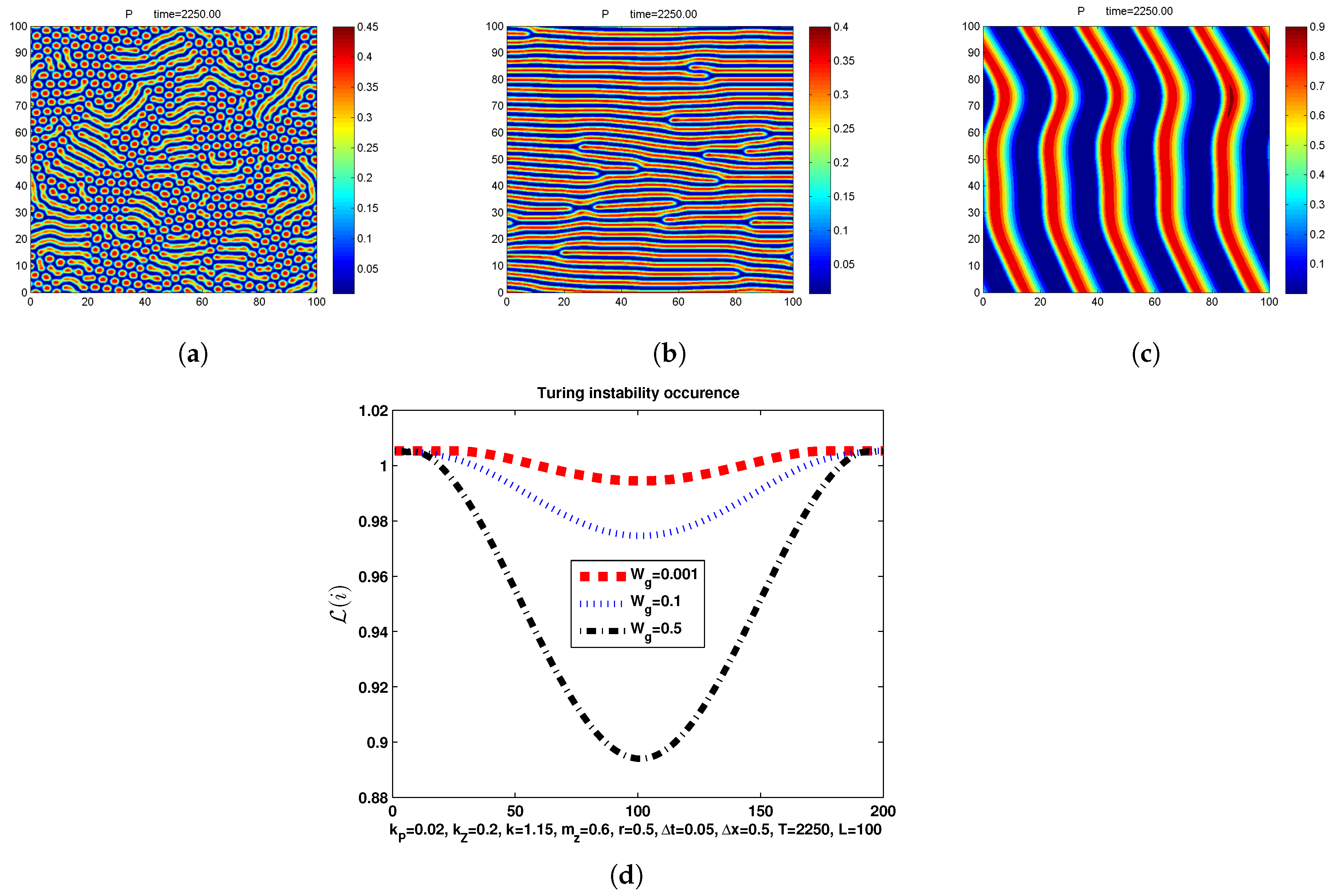
In Figure 2, in correspondence of parameters $k_P=0.02,k_Z=0.2,k=1.15,m_z=0.6,r=0.5$ and $T=2250,L=100$ we show the phytoplankton distribution P at $T=2250$ of the discrete $ADR$ model which proceeds with $\Delta t=0.05$ in the square ${[0,100]}^2$ discretized with $\Delta x=0.5$: we can observe the transition from hot spots-stripes to banded patterns obtained by increasing the advective coefficient $W_g$. In the same Figure we show that, in correspondence of that values of $W_g$, there is always a non empty set of wavenumbers where the occurrence condition for Turing instability is satisfied. In our simulations, we used Poisson Euler as discrete reaction semiflow; however, results remained unchanged if, in the third step of the algorithm described in Section 3.1, we use Explicit Euler in place of Poisson Euler to approximate the reaction step.

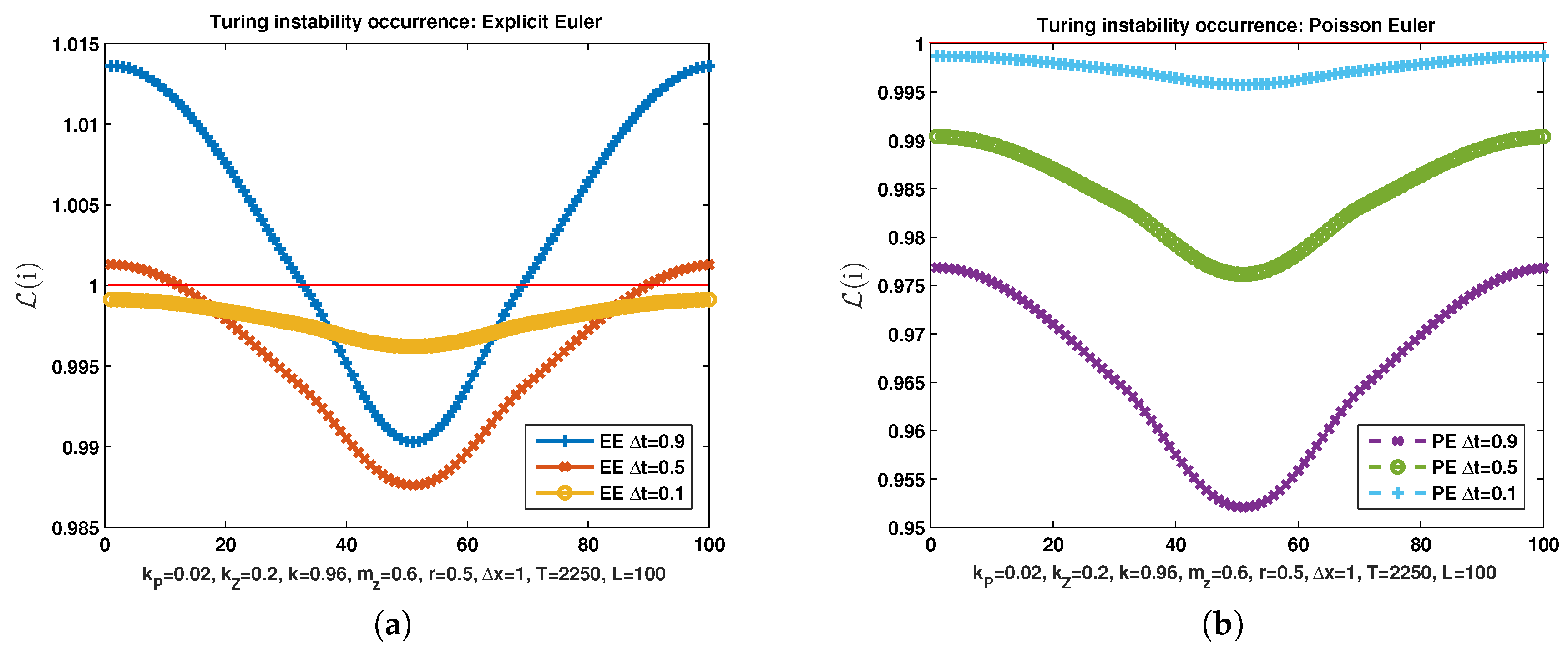
Now, set the parameters $k=0.96$ and $W_g=0.01$ and keep all the others unchanged. In Figure 3 we show the the Turing instability occurrence condition at $T=2250$ of the discrete $ADR$ model in the square ${[0,100]}^2$ discretized with $\Delta x=1$ and Explicit Euler semiflow (left) that proceeds with three different values of temporal stepsize $\Delta t=0.1,0.5,0.9$. While with larger values of the time step the Turing instability occurrence condition is satisfied, with $\Delta t=0.1$ the condition is not satisfied. This means that, if we want to infer the behaviour of the continuous model (9) with the ADR model, the explicit Euler discrete semiflow can give a wrong prediction if the temporal stepsize is not chosen sufficiently small.

With the same set of parameters, instead, Poisson Euler predicts the non occurrence of Turing instability even in correspondence of the largest stepsize $\Delta t=0.9$ (Figure 3b). This seems to indicate that using geometric numerical method to discretize a semiflow featured by a given structure (in this case the reaction semiflow featured by a Poisson structure) produces solutions qualitatively more similar to the solution of the theoretical flow.

3.3. Geometric Integration for the Spatiotemporal Dynamics of Aquatic Ecosystems

The spatiotemporal complexity of plankton and fish dynamics is explored in the seminal paper [29]. The authors show that the formation of a patchy spatial distribution of species can be described by a two-species prey-predator (i.e., Phytoplankton-Zooplankton) interaction modelled by the well-known Rosenzweig-MacArthur system [30], here given in non dimensional form:

$$\begin{array}{ccc}{\displaystyle \frac{\partial u}{\partial t}}\hfill & =\hfill & {\displaystyle D_u\Delta u+u(1-u)-\frac{uv}{\alpha +u}}\hfill \\ {\displaystyle \frac{\partial v}{\partial t}}\hfill & =\hfill & {\displaystyle D_v\Delta v+\frac{\beta uv}{\alpha +u}-\gamma v.}\hfill \end{array}$$

(10)

The populations are supposed distributed in an horizontal two-dimensional domain where zero-flux boundary conditions are set. The model (10) couples logistic prey growth with Holling II functional predator response and shows a very rich dynamics. Indeed, for a purely homogeneous initial distribution of species, the system stays homogeneous forever and no spatial pattern emerges; for a very weakly perturbed initial distribution, a smooth pattern arises that is not persistent and gradually evolves to the homogeneous distribution; for somehow stronger initial perturbations, the system evolves to the formation of a jagged spatial pattern which is persistent in time. The formation of the irregular patchy structure can be preceded by the evolution of a regular spiral spatial pattern.

Similarly to the well-known Rosenzweig-MacArthur model (10), the principal population dynamics models are based on logistic prey growth and ‘Holling type’ functional response of the predators [31]. They can exhibit spiral waves, target waves, and spatiotemporal chaos; for all those complex dynamics, the geometric numerical approach can represent a powerful tool to reproduce the correct behavior of the continuous solutions.

3.4. Positive Schemes for Spatially Extended Predator-Prey Dynamics

In this section, we focus on spatially-extended predator-prey models described by reaction–diffusion systems in the following general form

$$\begin{array}{cc}\hfill & \frac{\partial u}{\partial t}=f(u,v)+D_u\Delta u,\hfill \end{array}$$

(11)

$$\begin{array}{cc}\hfill & \frac{\partial v}{\partial t}=g(u,v)+D_v\Delta v,\hfill \end{array}$$

(12)

where $u(x,t)$ and $v(x,t)$ represent population densities of prey and predators at time t and position x and $D_u$ and $D_v$ are positive constant diffusion coefficients. The equations evolve in ${\Omega }_T:=\Omega \times (0,T)$ where the domain $\Omega$ is a bounded and open subset of ${\mathbb{R}}^d$, $d\le 3$. The system is augmented with initial conditions

$$u_0\left(x\right):=u(x,0),v_0\left(x\right):=v(x,0),x\in \Omega ,$$

(13)

and homogeneous zero-Neumann boundary conditions. To assure the non-negativity of solutions which correspond to biologically meaningful densities, the reaction kinetics have to satisfy [32]

$$\begin{array}{c}\hfill f(0,v),g(u,0)\ge 0,\forall u,v\ge 0.\end{array}$$

(14)

Consequently, if the initial data $(u_0\left(x\right),v_0\left(x\right))$ is chosen in ${[0,+\infty )}^2$ for all $x\in \Omega$, then by a maximum principle the solution $\left(u\right(x,t),v(x,t\left)\right)$ also lies in ${[0,+\infty )}^2$, which is a positively invariant region for the system. For the numerical approximation, in [23] a positive first order accurate integrator is obtained by compositions of exact and numerical flow. Firstly, the spatial discretization of the Laplacian operators transforms the problem (11) and (12) into the system

$${\displaystyle \frac{d\mathbf{y}}{dt}}=L_h\mathbf{y}+F_h\left(\mathbf{y}\right)$$

(15)

where $L_h=diag(D_u{\Delta }_h,D_v{\Delta }_h)$ represents an approximation of $L=diag(D_u\Delta ,D_v\Delta )$ on a grid ${\Omega }_h$ with a mesh width h. The solution $\mathbf{y}:={[{\mathbf{u}}_h,{\mathbf{v}}_h]}^T$ represents an approximate function of ${[u,v]}^T$ such that, for all $t\in [0,T]$, $\mathbf{y}\left(t\right)={[{\mathbf{u}}_h\left(t\right),{\mathbf{v}}_h\left(t\right)]}^T\in V_h\times V_h$, where $V_h$ is the vector space of all the functions from ${\Omega }_h$ to $\mathbb{R}$. For $t\in [0,T]$ and $F_h$ is the operator that associates to $\mathbf{y}\left(t\right)\in V_h\times V_h$ the function $F_h\left(\mathbf{y}\left(t\right)\right)\in V_h\times V_h$ defined as $F_h\left(\mathbf{y}\left(t\right)\right)\left(x\right)={[f\left({\mathbf{u}}_h\left(t\right)\left(x\right),{\mathbf{v}}_h\left(t\right)\left(x\right)\right),g\left({\mathbf{u}}_h\left(t\right)\left(x\right),{\mathbf{v}}_h\left(t\right)\left(x\right)\right)]}^T:={[f\left(u(x,t),v(x,t)\right),g\left(u(x,t),v(x,t)\right)]}^T$, for all $x\in {\Omega }_h.$

The diffusive flow ${\displaystyle \frac{d\mathbf{y}}{dt}}=L_h\mathbf{y}$ is supposed to be exactly computed being ${\phi }_{\Delta t}^{\left[D\right]}$ the exact flow. The reaction flow ${\displaystyle \frac{d\mathbf{y}}{dt}}=F_h\left(\mathbf{y}\right)$ is approximated by Poisson Euler schemes ${\Phi }_{\Delta t}^{\left[R\right]}$ in Equation (5), or the adjoint ${\Phi }_{\Delta t}^{\left[R\right]*}$ in Equation (7). Then the methods:

$${\Phi }_{\Delta t}={\Phi }_{\Delta t}^{\left[R\right]}\circ {\phi }_{\Delta t}^{\left[D\right]},{\Psi }_{\Delta t}={\phi }_{\Delta t}^{\left[D\right]}\circ {\Phi }_{\Delta t}^{\left[R\right]}$$

together with their adjoints

$${\Phi }_{\Delta t}^{*}={\phi }_{\Delta t}^{\left[D\right]}\circ {\Phi }_{\Delta t}^{\left[R\right]*},{\Psi }_{\Delta t}^{*}={\Phi }_{\Delta t}^{\left[R\right]*}\circ {\phi }_{\Delta t}^{\left[D\right]}.$$

are first order positive schemes, here denoted as EXponential-Positive Poisson (EXPP) schemes. For example, EXPP schemes defined by ${\Phi }_{\Delta t}^{*}={\phi }_{\Delta t}^{\left[D\right]}\circ {\varphi }_{\Delta t}^{\left[R\right]*}$, advances in time according to the steps:

$$\begin{array}{cccccc}{\displaystyle {\mathbf{u}}_h^{n_1}\left(x\right)}\hfill & =\hfill & {\displaystyle {\mathbf{u}}_h^n\left(x\right)e^{{\displaystyle \Delta t\frac{f({\mathbf{u}}_h^n\left(x\right),{\mathbf{v}}_h^{n_1}\left(x\right))}{{\mathbf{u}}_h^n\left(x\right)}}}x\in {\Omega }_h,}\hfill & {\displaystyle {\mathbf{u}}_h^{n+1}}\hfill & =\hfill & {\displaystyle e^{{\displaystyle \Delta t{D}_u{\Delta }_h}}{\mathbf{u}}_h^{n_1},}\hfill \\ {\displaystyle {\mathbf{v}}_h^{n_1}\left(x\right)}\hfill & =\hfill & {\displaystyle {\mathbf{v}}_h^n\left(x\right)e^{{\displaystyle \Delta t\frac{g({\mathbf{u}}_h^n\left(x\right),{\mathbf{v}}_h^{n_1}\left(x\right))}{{\mathbf{v}}_h^{n_1}\left(x\right)}}}x\in {\Omega }_h,}\hfill & {\displaystyle {\mathbf{v}}_h^{n+1}}\hfill & =\hfill & {\displaystyle e^{{\displaystyle \Delta t{D}_v{\Delta }_h}}{\mathbf{v}}_h^{n_1}}\hfill \end{array}$$

starting with ${\mathbf{u}}_h^0\left(x\right)={\mathbf{u}}_h\left(0\right)\left(x\right):=u(x,0)=u_0\left(x\right)$, and ${\mathbf{v}}_h^0\left(x\right)={\mathbf{v}}_h\left(0\right)\left(x\right):=v(x,0)=v_0\left(x\right)$ for all $x\in {\Omega }_h$. The above method, when applied for solving Rosenzweig-MacArthur model (10) reads as follows:

$$\begin{array}{cccccc}{\displaystyle {\mathbf{u}}_h^{n_1}\left(x\right)}\hfill & =\hfill & {\displaystyle e^{\Delta t}{\mathbf{u}}_h^n\left(x\right)e^{{\displaystyle \Delta t(1-{\mathbf{u}}_h^n\left(x\right))}}{e}^{{\displaystyle -\Delta t\frac{{\mathbf{v}}_h^{n_1}\left(x\right)}{{\mathbf{u}}_h^n\left(x\right)+\alpha }}}x\in {\Omega }_h,}\hfill & {\displaystyle {\mathbf{u}}_h^{n+1}}\hfill & =\hfill & {\displaystyle e^{{\displaystyle \Delta t{D}_u{\Delta }_h}}{\mathbf{u}}_h^{n_1},}\hfill \\ {\displaystyle {\mathbf{v}}_h^{n_1}\left(x\right)}\hfill & =\hfill & {\displaystyle e^{-\Delta t\gamma }{\mathbf{v}}_h^n\left(x\right)e^{{\displaystyle \Delta t\frac{\beta {\mathbf{u}}_h^n\left(x\right)}{{\mathbf{u}}_h^n\left(x\right)+\alpha }}}x\in {\Omega }_h,}\hfill & {\displaystyle {\mathbf{v}}_h^{n+1}}\hfill & =\hfill & {\displaystyle e^{{\displaystyle \Delta t{D}_v{\Delta }_h}}{\mathbf{v}}_h^{n_1}.}\hfill \end{array}$$

(16)

As we will see in the following, EXPP schemes outperform, in qualitative comparison, any existing scheme in detecting the onset of chaos predicted by model (10) for a test-case given in literature. A more general investigation on efficient positive approximations of the exponential flow ${\phi }_t^{\left[D\right]}$ (perfomed in [23] with polynomial Krylov approximation), together with a rigorous theoretical analysis, is still missing.

3.5. Implicit-Symplectic Schemes for Spatially Extended Predator-Prey Dynamics

Implicit-symplectic (IMSP) schemes are numerical integrators based on an implicit scheme for the stiff diffusive term and a geometric integrator for the reaction function. IMSP schemes were proposed in [33], as novel numerical schemes for the simulation of population and metapopulation predator–prey dynamics.

In order to illustrate the methods, consider the spatial semidiscretization of the Laplacian that yields to the system (15). The IMSP schemes are based on the expression of $F_h$ in (15) as the sum of two operators $F_h=f_h+g_h$, where for all t, $f_h\left(\mathbf{y}\left(t\right)\right),g_h\left(\mathbf{y}\left(t\right)\right)\in V_h\times V_h$ are defined as $f_h\left(\mathbf{y}\left(t\right)\right)\left(x\right)={[f\left({\mathbf{u}}_h\left(t\right)\left(x\right),{\mathbf{v}}_h\left(t\right)\left(x\right)\right),0]}^T$, $g_h\left(\mathbf{y}\left(t\right)\right)\left(x\right)={[0,g\left({\mathbf{u}}_h\left(t\right)\left(x\right),{\mathbf{v}}_h\left(t\right)\left(x\right)\right)]}^T$, for all $x\in {\Omega }_h.$ Then, for $i=1,2,3,$ define ${\mathbf{y}}_i$ such that $\mathbf{y}={\mathbf{y}}_1+{\mathbf{y}}_2+{\mathbf{y}}_3$ and satisfy

$$\begin{array}{c}{\displaystyle \frac{d{\mathbf{y}}_1}{dt}=L_h\left(\mathbf{y}\right),\frac{d{\mathbf{y}}_2}{dt}=f_h\left(\mathbf{y}\right),\frac{d{\mathbf{y}}_3}{dt}=g_h\left(\mathbf{y}\right).}\hfill \end{array}$$

A partitioned Runge-Kutta scheme is employed to solve the previous system: the dynamics of ${\mathbf{y}}_1$ is approximated by a diagonally implicit method, then the evolution of ${\mathbf{y}}_2$ and ${\mathbf{y}}_3$ variables is approximated by a partitioned symplectic Runge-Kutta method defined as

$$\begin{array}{cccc}\hfill & 0& & \\ \hfill & {\beta }_1& {\alpha }_1& & \\ \hfill & ⋮& ⋮& & \ddots & \\ \hfill & {\beta }_1& {\alpha }_1& \cdots & \cdots & 0\\ \hfill & {\beta }_1& {\alpha }_1& \cdots & \cdots & {\beta }_s& {\alpha }_s\\ \hfill & {\beta }_1& {\alpha }_1& \cdots & \cdots & {\beta }_s& {\alpha }_s\end{array}\begin{array}{cccc}\hfill & {\beta }_1& & \\ \hfill & {\beta }_1& 0& & \\ \hfill & ⋮& ⋮& & \ddots & \\ \hfill & {\beta }_1& {\alpha }_1& \cdots & \cdots & {\beta }_s\\ \hfill & {\beta }_1& {\alpha }_1& \cdots & \cdots & {\beta }_s& 0\\ \hfill & {\beta }_1& {\alpha }_1& \cdots & \cdots & {\beta }_s& {\alpha }_s\end{array}$$

(17)

In [33] the authors set $s=1$ in (17) and apply the following two-stage schemes

$$\begin{array}{ccc}0& 0& 0\\ \alpha +\beta & \alpha & \beta \\ & \alpha & \beta \end{array}\begin{array}{ccc}0& 0& 0\\ \alpha +\beta & \beta & \alpha \\ & \beta & \alpha \end{array}\begin{array}{ccc}\beta & \beta & 0\\ \beta \hfill & \beta & 0\\ \hfill & \beta & \alpha \end{array}$$

in order to approximate ${\mathbf{y}}_1$, ${\mathbf{y}}_2$ and ${\mathbf{y}}_3$, respectively. The resulting method for the approximation of $\mathbf{y}={[{\mathbf{u}}_h,{\mathbf{v}}_h]}^T$ is given by

$$\begin{array}{c}{\displaystyle \frac{{\mathbf{Y}}_h^{n,1}-{\mathbf{y}}_h^n}{\Delta t}}=\beta g_h\left({\mathbf{Y}}_h^{n,1}\right),\hfill \\ {\displaystyle \frac{{\mathbf{Y}}_h^{n,2}-{\mathbf{Y}}_h^{n,1}}{\Delta t}}-\alpha L_h{\mathbf{Y}}_h^{n,1}=\beta f_h\left({\mathbf{Y}}_h^{n,1}\right),\hfill \\ {\displaystyle \frac{{\mathbf{Y}}_h^{n,3}-{\mathbf{Y}}_h^{n,2}}{\Delta t}}-\beta L_h{\mathbf{Y}}_h^{n,3}=\alpha f_h\left({\mathbf{Y}}_h^{n,3}\right),\hfill \\ {\displaystyle \frac{{\mathbf{y}}^{n+1}-{\mathbf{Y}}_h^{n,3}}{\Delta t}}=\alpha g_h\left({\mathbf{Y}}_h^{n,3}\right).\hfill \end{array}$$

(18)

where ${\mathbf{y}}^n\in V_h$ approximates $\mathbf{y}\left(t_n\right)$, for $t_n=t_0+n\Delta t$ and ${\mathbf{Y}}_h^{n,1},{\mathbf{Y}}_h^{n,2},{\mathbf{Y}}_h^{n,3}\in V_h$ are intermediate steps. For $\beta =1$ and $\alpha =0$ this scheme is featured by first order approximation; when $\beta =\alpha =1/2$, then it is a second order accurate method. Moreover, under the assumption that diffusivity coefficients $D_u$ and $D_v$ nullify, the first order scheme represents a symplectic Euler scheme which handles the variable ${\mathbf{u}}_h$ in an explicit way and the variable ${\mathbf{v}}_h$ implicitly. The second order approximation reduces to the classical Störmer–Verlet scheme when it is written as a partitioned Runge-Kutta method exploiting the trapezoidal rule in order to approximate the stiff diffusive term.

In terms of ${\mathbf{u}}_h$ and ${\mathbf{v}}_h$, the first order IMSP scheme, when applied to the Rosenzweigh–MacArthur model (10) reads

$$\begin{array}{cc}{\displaystyle \frac{{\mathbf{u}}_h^{n_1}\left(x\right)-{\mathbf{u}}_h^n\left(x\right)}{\Delta t}={\mathbf{u}}_h^n\left(x\right)(1-{\mathbf{u}}_h^n\left(x\right))-\frac{{\mathbf{u}}_h^n\left(x\right){\mathbf{v}}_h^{n_1}\left(x\right)}{\alpha +{\mathbf{u}}_h^n\left(x\right)}x\in {\Omega }_h,}\hfill & {\displaystyle \frac{{\mathbf{u}}_h^{n+1}-{\mathbf{u}}_h^{n_1}}{\Delta t}=D_u{\Delta }_h{\mathbf{u}}_h^{n+1},}\hfill \\ {\displaystyle \frac{{\mathbf{v}}_h^{n_1}\left(x\right)-{\mathbf{v}}_h^n\left(x\right)}{\Delta t}=\beta \frac{{\mathbf{u}}_h^n\left(x\right){\mathbf{v}}_h^{n_1}\left(x\right)}{\alpha +{\mathbf{u}}_h^n\left(x\right)}-\gamma {\mathbf{v}}_h^{n_1}\left(x\right)x\in {\Omega }_h,}\hfill & {\displaystyle \frac{{\mathbf{v}}_h^{n+1}-{\mathbf{v}}_h^{n_1}}{\Delta t}=D_v{\Delta }_h{\mathbf{v}}_h^{n+1}.}\hfill \end{array}$$

(19)

3.5.1. A Linear Stability Analysis

A stability analysis of IMSP schemes in terms of the diffusion and the reaction time-scales was recently developed in [34]. Their numerical simulations reveal that IMSP schemes provide the best choice for spatio-temporal dynamics of standing oscillations around an equilibrium of centre type. Their dissipation analysis is based on the application of IMSP schemes to the ODE test system:

$$\begin{array}{cc}\hfill & \frac{du}{dt}=-\beta v+\lambda u,\frac{dv}{dt}=\beta u+\lambda v.\hfill \end{array}$$

The first order IMSP scheme (19), introduced in [33], which approximate the diffusive term related to the coefficient $\lambda$ with implicit Euler and the reaction term with symplectic Euler, can be written as

$$\begin{array}{cc}\hfill & \frac{u^{n_1}-u^n}{\Delta t}=-\beta v^{n_1},\frac{v^{n_1}-v^{n_1}}{\Delta t}=\beta u^n\hfill \\ \hfill & \frac{u^{n+1}-u^{n_1}}{\Delta t}-\lambda u^{n+1}=0,\frac{v^{n+1}-v^{n_1}}{\Delta t}-\lambda v^{n+1}=0.\hfill \end{array}$$

By eliminating $u^{n_1}$ and $v^{n_1}$ and setting $\xi =\lambda \Delta t$, $\nu =\beta \Delta t$ the numerical solution can be written as

$$\left(\begin{array}{c}{u}^{n+1}\\ v^{n+1}\end{array}\right)=M\left(\begin{array}{c}{u}^n\hfill \\ v^n\hfill \end{array}\right),M={\displaystyle \frac{1}{1-\xi }}\left(\begin{array}{cc}1-{\nu }^2& -\nu \\ \nu & 1.\end{array}\right)$$

By denoting with ${\lambda }_M^{\pm }={\rho }_M{e}^{\pm i{\theta }_M}$ the eigenvalues of M, and comparing the numerical with the exact solution written as

$$\left(\begin{array}{c}u\left(t_{n+1}\right)\hfill \\ v\left(t_{n+1}\right)\hfill \end{array}\right)=e^{\xi }\left(\begin{array}{cc}cos\left(\nu n\right)\hfill & -sin\left(\nu n\right)\hfill \\ sin\left(\nu n\right)\hfill & cos\left(\nu n\right)\hfill \end{array}\right)\left(\begin{array}{c}u\left(t_n\right)\hfill \\ v\left(t_n\right)\hfill \end{array}\right),$$

where the quantities $\delta (\xi ,\nu )=e^{\xi }-{\rho }_M(\xi ,\nu )$ and $\varphi (\xi ,\nu )=\nu -{\theta }_M(\xi ,\nu )$ represent the dissipative and dispersion errors, respectively. Since $\xi <0$, we require that the IMSP method is dissipative i.e., ${\rho }_M(\xi ,\nu )<1$. Since the eigenvalues of M are

$${\lambda }_M^{\pm }={\displaystyle \frac{2-{\nu }^2\pm \sqrt{({\nu }^2-2)-4}}{2(1-\xi )}}$$

then ${\rho }_M(\xi ,\nu )<1$ if and only if ${\nu }^2<{\displaystyle \frac{{(\xi -2)}^2}{1-\xi }}$.

To study the dispersion properties of the IMSP method firstly we notice that ${\lambda }_M^{\pm }={\rho }_{M}cos\left({\theta }_M\right)\pm isin\left({\theta }_M\right)$ with $cos\left({\theta }_M\right)={\displaystyle \frac{trace\left(M\right)}{2\sqrt{det\left(M\right)}}}$. The dispersion error is calculated by

$$\varphi (\xi ,\nu )=\nu -arccos{\displaystyle \frac{trace\left(M\right)}{2\sqrt{det\left(M\right)}}}=\nu -arccos{\displaystyle \frac{2-{\nu }^2}{2\sqrt{1-\xi }}}$$

It results that $\varphi (\xi ,\nu )=-{\nu }^3/24+O\left({\nu }^5\right)$ for $\xi \to 0$, with a constant error smaller than that of the explicit ADI scheme and of IMplicit-EXplicit (IMEX)-Euler scheme [34].

3.5.2. Analysis of Semi-Discrete in Time IMSP First Order Scheme in Weak Form

The results of a more technical methodology based on the analysis of a semi-discrete in time formulation of IMSP schemes has been performed in [32]. Let $D=diag(D_u,D_v)$ be a linear matrix operator and consider the vector $G\left(y\right)={[f(u,v),g(u,v)]}^T$. With the previous notations, the system (11)–(12) leads to the following continuous-in-time weak formulation: find $y(·,t)=[u(·,t),v(·,t)]\in H^1(\Omega )\times H^1(\Omega )$ such that

$$\begin{array}{cc}\hfill & \left(y_t,\chi \right)+(D\nabla y,\nabla \chi )=(G\left(y\right),\chi )\hfill \end{array}$$

(20)

for all $\chi \in H^1(\Omega )\times H^1(\Omega )$ and for almost every $t\in (0,T)$. Define the vectors $G^{\left(u\right)}={[f(u,v),0]}^T$ and $G^{\left(v\right)}={[0,g(u,v)]}^T$; then IMSP scheme (in weak form) is defined as follows: for $n=0,\cdots ,N-1$, find $y^{n_1},y^{n_2},y^{n_3},y^{n+1}\in H^1(\Omega )\times H^1(\Omega )$ such that $\forall \chi \in H^1(\Omega )\times H^1(\Omega )$:

$$\begin{array}{cc}\hfill & \left(\frac{y^{n_1}-y^n}{\Delta t},\chi \right)=\beta \left(G^{\left(v\right)}\left(y^{n_1}\right),\chi \right)\hfill \\ \hfill & \left(\frac{y^{n_2}-y^{n_1}}{\Delta t},\chi \right)+\alpha (D\nabla y^{n_1},\nabla \chi )=\beta \left(G^{\left(u\right)}\left(y^{n_1}\right),\chi \right)\hfill \\ \hfill & \left(\frac{y^{n_3}-y^{n_2}}{\Delta t},\chi \right)+\beta (D\nabla y^{n_3},\nabla \chi )=\alpha \left(G^{\left(u\right)}\left(y^{n_3}\right),\chi \right)\hfill \\ \hfill & \left(\frac{y^{n+1}-y^{n_3}}{\Delta t},\chi \right)=\alpha \left(G^{\left(v\right)}\left(y^{n_3}\right),\chi \right).\hfill \end{array}$$

For $\beta =1$ and $\alpha =0$ we recover the first-order accurate IMSP scheme. In terms of the variables u and v, it can be written as follows. For $n=0,\cdots ,N-1$, find $v^{n_1}$, $u^{n_1}$, $v^{n+1}$, $u^{n+1}\in H^1(\Omega )$ such that for all $\chi \in H^1(\Omega )$

$$\begin{array}{c}{\displaystyle \left(\frac{u^{n_1}-u^n}{\Delta t},\chi \right)=\left(f(u^n,v^{n_1}),\chi \right),\left(\frac{v^{n_1}-v^n}{\Delta t},\chi \right)=\left(g(u^n,v^{n_1}),\chi \right)}\hfill \\ {\displaystyle \left(\frac{u^{n+1}-u^{n_1}}{\Delta t},\chi \right)+D_u(\nabla u^{n+1},\nabla \chi )=0,\left(\frac{v^{n+1}-v^{n_1}}{\Delta t},\chi \right)+D_v(\nabla v^{n+1},\nabla \chi )=0,}\hfill \end{array}$$

(21)

where we adopted a uniform mesh grid of $N+1$ points $t_n=n\Delta t$, $n=0,\cdots ,N$ with constant time step $\Delta t=T/N$ to discretize the temporal horizon $(0,T)$. Moreover, $v^0=v_0(·)$ and $u^0=u_0(·)$ are the initial densities of predators and prey respectively.

We summarize the main theoretical results proven in [32] obtained under the assumptions that $f(u,v)$ has logistic dominated growth in the first variable, namely

$$\begin{array}{c}\hfill f(u,v)\le u(1-u),\forall u,v\ge 0,\end{array}$$

(22)

and the function g satisfies a sub-linear growth in the second variable, i.e., there exists $C_g>0$ such that

$$\begin{array}{c}\hfill g(u,v)\le C_{g}v,\forall u,v\ge 0.\end{array}$$

(23)

Theorem 3

(Positivity). Assume the time step $\Delta t<1/L$ and Ω is a domain of class $C^1$. Provided that the initial conditions are positive, i.e., $u_0\left(x\right)=u(x,0)>0,v_0\left(x\right)=v(x,0)>0$, for all $x\in \Omega$, then the solutions $u^n\left(x\right),v^n\left(x\right)$ of the first-order scheme (21) are positive for all $n\ge 0$.

Theorem 4

(Stability). Assume the time step satisfies $\Delta t\le 1/max\left\{1,2C_g\right\}$. Then the solution to (21) satisfies the following energy estimate:

$$\begin{array}{cc}\hfill & \parallel u^N{\parallel }^2+{\parallel v^N\parallel }^2+\sum _{n=0}^{N-1}\left(\parallel u^{n+1}-u^n{\parallel }^2+\frac{1}{2}{\parallel v^{n+1}-v^n\parallel }^2\right)\hfill \\ \hfill & +\Delta t\sum _{n=0}^{N-1}\left(2D_u\parallel \nabla u^{n+1}{\parallel }^2+D_v{\parallel \nabla v^{n+1}\parallel }^2\right)\hfill \\ \hfill & \le exp\left(\frac{2\Delta tN}{\Delta t_s-\Delta t}\right)\left(\parallel u_0{\parallel }^2+{\parallel v_0\parallel }^2\right).\hfill \end{array}$$

(24)

Theorem 5

(Error estimate). Let ${\epsilon }_u^n,{\epsilon }_v^n\in {\left(H^1(\Omega )\right)}^{\prime }$ denote the following local truncation errors for scheme (21), satisfying

$$\begin{array}{cc}\hfill & \langle {\epsilon }_u^n,\chi \rangle :=\frac{1}{\Delta t}\langle u\left(t_n\right)-u\left(t_{n-1}\right),\chi \rangle -\langle f(u\left(t_{n-1}\right),v\left(t_n\right)),\chi \rangle +D_u(\nabla u\left(t_n\right),\nabla \chi ),\hfill \\ \hfill & \langle {\epsilon }_v^n,\chi \rangle :=\frac{1}{\Delta t}\langle v\left(t_n\right)-v\left(t_{n-1}\right),\chi \rangle -\langle g(u\left(t_{n-1}\right),v\left(t_n\right)),\chi \rangle +D_v(\nabla v\left(t_n\right),\nabla \chi ),\hfill \end{array}$$

where $\chi \in H^1(\Omega )$. Furthermore, let $e_u^n,e_v^n\in H^1(\Omega )$ denote the point-wise errors

$$\begin{array}{c}\hfill e_u^n=u\left(t_n\right)-u^n,e_v^n=v\left(t_n\right)-v^n,\end{array}$$

satisfying the following equations:

$$\begin{array}{cc}\hfill & \frac{e_u^{n+1}-e_u^n}{\Delta t}-D_u{\Delta }_h{e}_u^{n+1}=f(u\left(t_n\right),v\left(t_{n+1}\right))-f(u^n,v^{n_1})+{\epsilon }_u^{n+1},\hfill \\ \hfill & \frac{e_v^{n+1}-e_v^n}{\Delta t}-D_v{\Delta }_h{e}_v^{n+1}=g(u\left(t_n\right),v\left(t_{n+1}\right))-g(u^n,v^{n_1})+{\epsilon }_v^{n+1}.\hfill \end{array}$$

Assume the classical solution of (11) and (12) has the following regularity:

$$\begin{array}{c}\hfill \frac{du}{dt},\frac{dv}{dt},\frac{d^{2}u}{d{t}^2},\frac{d^{2}v}{d{t}^2}\in L^2(0,T,{\left(H^1(\Omega )\right)}^{\prime }).\end{array}$$

and assume the nonlinearities $f,g$ are globally Lipschitz, i.e., there exists $L>0$ such that

$$\begin{array}{c}\hfill |f(u_1,v_1)-f(u_2,v_2)|+|g(u_1,v_1)-g(u_2,v_2)|\le L(|u_1-u_2|+|v_1-v_2\left|\right)\end{array}$$

for all $u_i$ and $v_i$ in a compact subset of ${\mathbb{R}}^{+}\times {\mathbb{R}}^{+}$. Then, there exists a constant $C(u,v)>0$ such that

$$\begin{array}{cc}\hfill & \underset{0\le n\le N}{max}\left(\parallel e_u^n\parallel +\parallel e_v^n\parallel \right)+{\left(\Delta t\sum _{n=0}^{N-1}\left(D_u\parallel \nabla e_u^{n+1}{\parallel }^2+D_v{\parallel \nabla e_v^{n+1}\parallel }^2\right)\right)}^{\frac{1}{2}}\hfill \\ \hfill & \le C(u,v)\left(\parallel e_u^0\parallel +\parallel e_v^0\parallel +\Delta t\right).\hfill \end{array}$$

The above error estimate implies convergence and first-order accuracy in time for the solution $u^n,v^n$ of Equation (21) with the assumption that $e_u^0,e_v^0$ are also of order $\Delta t$.

3.6. Numerical Comparison between IMEX and Geometric Integrators

Consider the dynamics of Equation (10) evolving in the horizontal layer $\Omega =[0,900]\times [0,300]$ with parameters $\alpha =0.4$, $\beta =2$, $\gamma =0.6$. Initial conditions are set as

$$\begin{array}{ccc}{u}_0\left(x\right)=u_0(X,Y)\hfill & =\hfill & 6/35-2·{10}^{-7}(X-180)(X-720)-6·{10}^{-7}(Y-90)(Y-210)\hfill \\ v_0\left(x\right)=v_0(X,Y)\hfill & =\hfill & 116/245-3·{10}^{-5}(X-450)-6·{10}^{-5}(Y-135).\hfill \end{array}$$

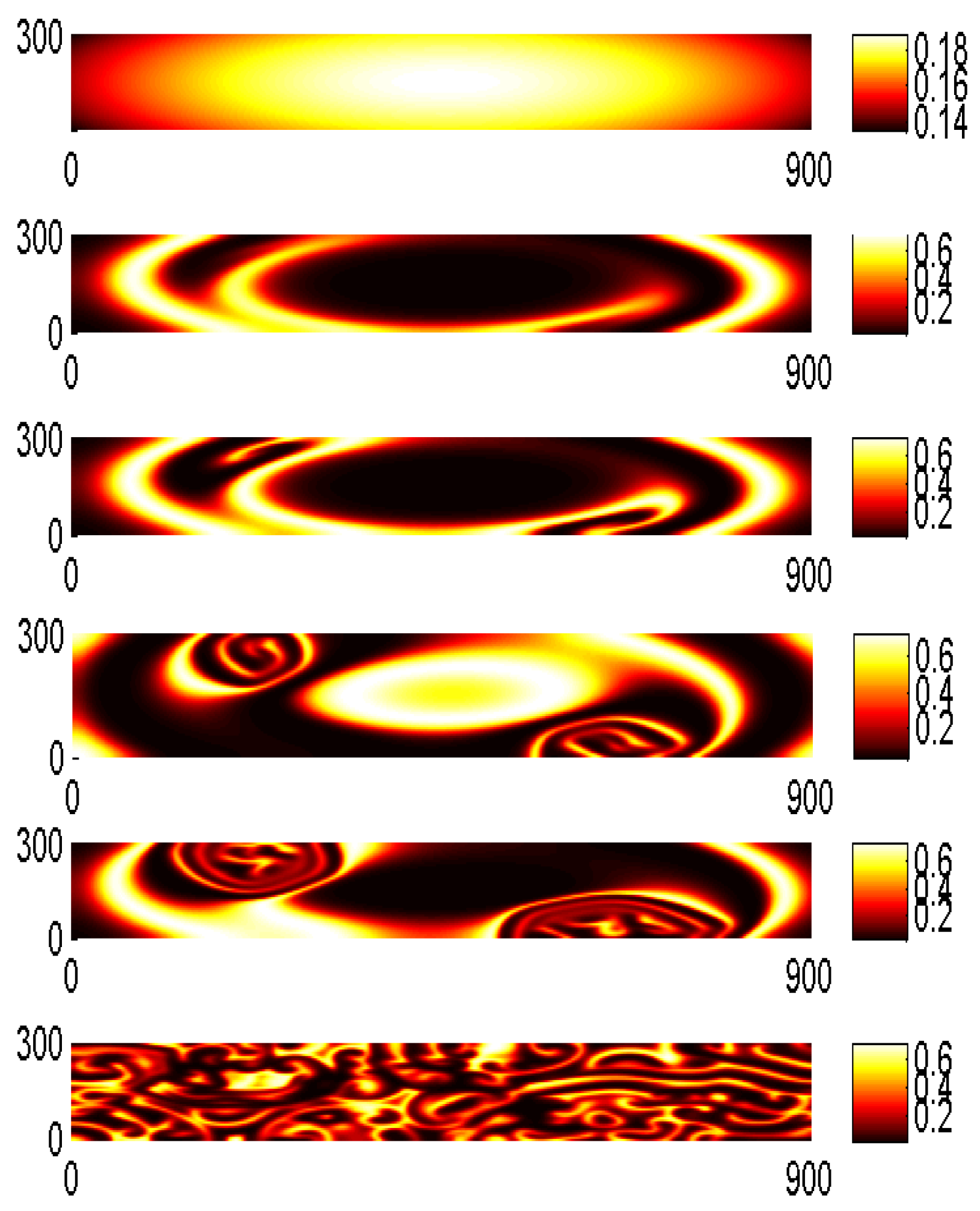
The five-point central difference approximation of the Laplacian in two dimensions on a grid ${\Omega }_h$ with stepsize $h=1$ was used. The spatially explicit dynamics of the phytoplankton-zooplankton model is shown in Figure 4 where the prey (u) approximations obtained with first order EXPP method given in Equation (16) are plotted. We see that spirals appear with their centers located in the vicinity of equilibria $u^{*}=6/35$ and $v^{*}=116/245$ of the dynamics. At $t=300$ (see Figure 4) we observe the onset of destruction of the spirals which leads to the formation of two growing embryos of the patchy spatial pattern and finally, at $t=1200$, the irregularities occupy the whole domain. In [29] the onset of the spatial patterns near the critical points is already evident at $t=120$.

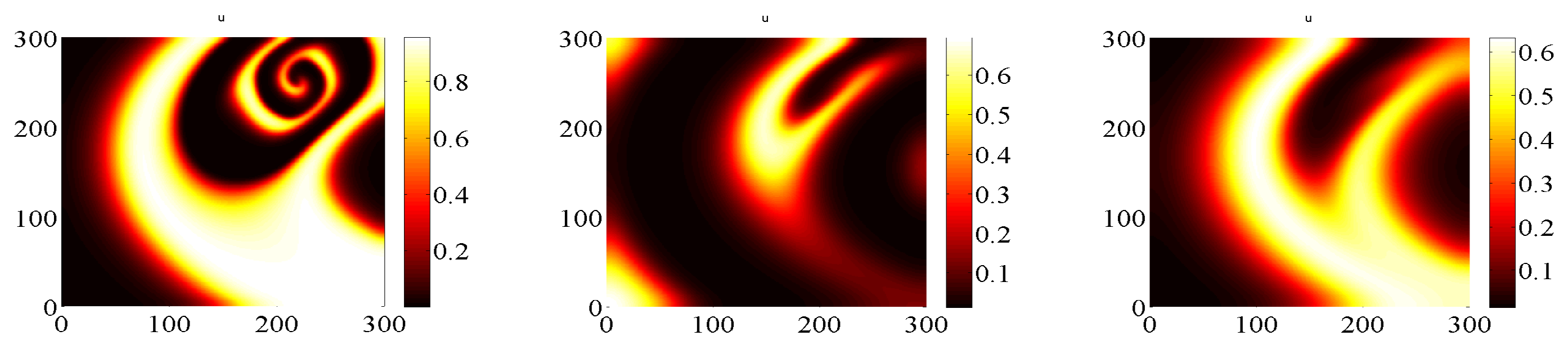
To explain such a difference in the transient to the formation of irregular patchy spatial patterns the dynamics evolution in the temporal interval $\left[0120\right]$ in a smaller domain $\Omega =[0,300]\times [0,300]$ was considered. The IMEX first order scheme

$$\begin{array}{cc}{\displaystyle \frac{{\mathbf{u}}_h^{n_1}\left(x\right)-{\mathbf{u}}_h^n\left(x\right)}{\Delta t}={\mathbf{u}}_h^n\left(x\right)(1-{\mathbf{u}}_h^n\left(x\right))-\frac{{\mathbf{u}}_h^n\left(x\right){\mathbf{v}}_h^n\left(x\right)}{\alpha +{\mathbf{u}}_h^n\left(x\right)}x\in {\Omega }_h,}\hfill & {\displaystyle \frac{{\mathbf{u}}_h^{n+1}-{\mathbf{u}}_h^{n_1}}{\Delta t}=D_u{\Delta }_h{\mathbf{u}}_h^{n+1},}\hfill \\ {\displaystyle \frac{{\mathbf{v}}_h^{n_1}\left(x\right)-{\mathbf{v}}_h^n\left(x\right)}{\Delta t}=\beta \frac{{\mathbf{u}}_h^n\left(x\right){\mathbf{v}}_h^n\left(x\right)}{\alpha +{\mathbf{u}}_h^n\left(x\right)}-\gamma {\mathbf{v}}_h^n\left(x\right)x\in {\Omega }_h,}\hfill & {\displaystyle \frac{{\mathbf{v}}_h^{n+1}-{\mathbf{v}}_h^{n_1}}{\Delta t}=D_v{\Delta }_h{\mathbf{v}}_h^{n+1}.}\hfill \end{array}$$

(25)

was compared with EXPP in (16) and IMSP given in (19). The results are shown in Figure 5, Figure 6 and Figure 7 and summarized below.

• For IMEX and IMSP schemes (Figure 5 and Figure 6) we start with a temporal stepsize $\Delta t=1/3$ (in order to have convergence) and then we reduce the stepsize. As $\Delta t$ is reduced, the initial spiral patterns generated by the IMEX scheme with large temporal stepsize disappear, thus confirming that the spiral pattern in [29] is a numerical artifact.
• This is not the case of EXPP method (Figure 7), which exhibits no spiral, even with the larger initial stepsize $\Delta t=1$. By reducing the stepsize the solution does not change significantly, with this meaning that convergence is reached and no artifacts arised.

As a conclusion, we have observed that a numerical method applied to the Rosenzweig-MacArthur model (10), may alter the solution in the short run. To make correct qualitative considerations on the transient dynamics, classical methods as IMEX scheme need a very small stepsize. Geometric IMSP and EXPP schemes both show a more stable behaviour; however, the positive EXPP scheme provides the best performance.

4. Symplectic-Exponential Lawson Integration for the Control of Invasive Population

Mathematical modeling and optimization play an important role in improving strategies for the control and eradication of invasive species [15,35,36], a crucial aspect in nature conservation [37].

In [16], a reaction-diffusion partial differential equation models the spatiotemporal dynamics of the invasion of alien fish population inside a very complex geometry representing a realistic lake and the optimal control theory has been applied to obtain the optimal management strategy with a given budget constraint. The model describes a complex and realistic situation by including a control term that has Holling-II type behavior, a budget constraint and the habitat suitability function which represents the suitability of habitat for a given species based on known affinities with environmental parameters.

The goal is to minimize the environmental damage over time at the minimum cost, in terms of the resources allocated to the species harvesting. The objective function is a sum of three terms. The first term takes into account of the environmental damage through the function $\omega (x,t)>0$ over $\Omega \times [0,T]$, $\omega \in L^{\infty }(\Omega \times [0,T])$, which is assumed to have a cost which increases with the presence of the invasive species:

$$\begin{array}{c}\hfill {\displaystyle J_1={\int }_{\Omega \times [0,T]}{e}^{-\delta t}\omega \left(x,t\right)udxdt+{\int }_{\Omega }\nu \left(x\right)u\left(x,T\right)dx.}\end{array}$$

where $u(x,t)$ represents the population density at time $t\in [0,T]$ and (vector) position x in an open bounded $\nu \in L^{\infty }(\Omega )$, $\nu \left(x\right)\ge 0$ is a weight for the final population density and $\delta \in (0,1)$ is the discount factor. The second term is the cost due to the control effort:

$$\begin{array}{c}\hfill {\displaystyle J_2={\int }_{\Omega \times [0,T]}{e}^{-\delta t}E{\left(x,t\right)}^{2}dxdt.}\end{array}$$

The third term accounts for the budget constraint $0<E<B$ introduced as a penalty term with weight $c\ge 0$;

$$\begin{array}{c}\hfill {\displaystyle J_3=c{\int }_{\Omega \times [0,T]}{e}^{-\delta t}{\left(\frac{E\left(x,t\right)}{B}\right)}^{3}dxdt.}\end{array}$$

The optimal control model searches for a control

$$E^{*}\in \mathcal{U}=\{E\in L^{\infty }(\Omega \times [0,T]):0\le E(x,t)\le B\mathrm{for} \mathrm{all} (x,t)\in \Omega \times [0,T]\}$$

such that $J\left(E^{*}\right)={min}_{E\in \mathcal{U}}J\left(E\right)$, subjects to the state equation

$$\begin{array}{ccc}\hfill {\displaystyle \frac{\partial u}{\partial t}(x,t)}& -& D\Delta u(x,t)=ru(x,t)\left(\rho \left(x\right)-\frac{u(x,t)}{k}\right)-\frac{\mu u(x,t)E(x,t)}{1+h\mu u(x,t)},\hfill \\ \hfill \\ \hfill u(x,0)& =& u_0\left(x\right),on\Omega ,\nabla u(x,t)·\widehat{\mathbf{n}}=0,on\partial \Omega \times [0,T],\hfill \end{array}$$

where $D>0$ represents the constant diffusion coefficient and $\widehat{\mathbf{n}}$ is the outward normal vector on $\partial \Omega$. The term $\rho \left(x\right)$ represents the habitat suitability function which is bounded $\rho \left(x\right)\in [0,1]$ for each $x\in \Omega$; that implies $\rho \in L^{\infty }(\Omega )$ and ${\parallel \rho \parallel }_{L^{\infty }(\Omega )}\le 1$. Under the assumption that $u_0\in H^1(\Omega )$ the usual Sobolev space (with its dual $H^1{(\Omega )}^{*}$), the solution of the problem (26)-(26), is to be considered in week sense that is $u\in L^2(0,T;H^1(\Omega ))$ such that $\frac{\partial u}{\partial t}\in L^2(0,T;H^1{(\Omega )}^{*})$ and

$$\begin{array}{c}{\displaystyle {\int }_{\Omega }\frac{\partial u}{\partial t}\chi d\mathbf{x}+{\int }_{\Omega }D\nabla u·\nabla \chi d\mathbf{x}={\int }_{\Omega }\left(r\rho -\frac{ru}{k}-\frac{\mu E(x,t)}{1+h\mu u}\right)u\chi d\mathbf{x},}\end{array}$$

for almost every $t\in [0,T]$ and for any test function $\chi \in H^1(\Omega )$ [16].

The optimality conditions yield the following boundary value system

$$\begin{array}{ccc}\hfill & \hfill & {\displaystyle \frac{\partial u}{\partial t}=D\Delta u+ru\left(\rho -\frac{u}{k}\right)-\frac{\mu uE}{1+h\mu u},}\hfill \\ \hfill & \hfill & {\displaystyle \frac{\partial \lambda }{\partial t}=-D\Delta \lambda +(\delta -r\rho )\lambda +\frac{2ru\lambda }{k}+\frac{\mu \lambda E}{{(1+h\mu u)}^2}-\omega ,}\hfill \\ \hfill & \hfill & u\left(x,0\right)=u_0\left(x\right),\mathrm{on} \Omega ,\nabla u·\widehat{\mathbf{n}}=0,\mathrm{on} \partial \Omega \times [0,T],\hfill \\ \hfill & \hfill & \lambda \left(x,T\right)=\nu \left(x\right),\mathrm{on} \Omega ,\nabla \lambda ·\widehat{\mathbf{n}}=0,\mathrm{on} \partial \Omega \times [0,T],\hfill \end{array}$$

(26)

equipped with

$$E(\mathbf{x},t)=min\{max\{\phi \left(u\right(x,t),\lambda (x,t\left)\right),0\},B\},\mathrm{on} \Omega \times [0,T],$$

where

$${\displaystyle \phi (u,\lambda )=\left\{\begin{array}{cc}{\displaystyle \frac{B^3}{3c}\left(\sqrt{1+\frac{3c\mu u\lambda }{B^3(1+h\mu u)}}-1\right),}\hfill & \mathrm{if} c>0,\hfill \\ {\displaystyle \frac{\mu u\lambda }{2(1+h\mu u)},}\hfill & \mathrm{if} c=0.\hfill \end{array}\right.}$$

(27)

As before, the approximation process of the whole dynamics assumes a semi-discretization in the space variable; the resulting procedure leads to a boundary value problem governed by the ordinary differential system (15) in the time variable, which can be numerically integrated by a partitioned method which consists of a Runge-Kutta scheme and the exponential Lawson algorithm [38] related to the symplectic counterpart [39].

4.1. Exponential Lawson Symplectic Integration of the Reaction Semiflow

We illustrate the advantage of using a symplectic numerical scheme when we approximate the boundary value problem described by the reaction semiflow. For simplicity, we assume $\rho =1$ and $\nu >0$ and $\omega >0$ as constant functions. Consider the boundary value ODE system:

$$\begin{array}{c}{\displaystyle \frac{du}{dt}=ru\left(1-\frac{u}{k}\right)-\frac{\mu uE}{1+h\mu u},}\hfill \end{array}$$

(28)

$$\begin{array}{c}{\displaystyle \frac{d\lambda }{dt}=\delta \lambda +\left(-r+\frac{2ru}{k}+\frac{\mu E}{{(1+h\mu u)}^2}\right)\lambda -\omega ,}\hfill \end{array}$$

(29)

with $u\left(0\right)=u_0$ and $\lambda \left(T\right)=\nu$, equipped with

$$E=min\left\{max\left\{\phi (u,\lambda ),0\right\},B\right\},\mathrm{for} t\in [0,T],$$

and $\phi (u,\lambda )$ is defined in (27). We use the forward-backward sweep approach described in [40] joint with an exponential Lawson symplectic scheme [39]. This choice is motivated by the fact that, for all $x\in {\Omega }_h$ the ODE system (28) and (29) is what is referred in literature as a nearly Hamiltonian system :

$${\displaystyle \frac{du}{dt}=\frac{\partial H(u,\lambda )}{\partial \lambda },\frac{d\lambda }{dt}=\delta \lambda -\frac{\partial H(u,\lambda )}{\partial u}.}$$

where

$$H(u,\lambda )=\left({\displaystyle ru\left(1-\frac{u}{k}\right)-\frac{\mu uE}{1+h\mu u}}\right)\lambda +\omega u.$$

It has been proven that a partitioned method which consists of a Runge-Kutta scheme for the state variable and the exponential Lawson [38] symplectic counterpart for the current costate, is an effective alternative to the standard ODE solvers in the framework of optimal control [39].

In more details, given a Runge-Kutta scheme defined by coefficients $a_{i,j}$, $b_i$, with $b_i\ne 0$ and its symplectic counterpart defined by coefficients ${\widehat{a}}_{i,j}$, $b_i$, with $b_k{b}_j=b_k{\widehat{a}}_{kj}+b_j{a}_{jk}$ for each $k,j$ and $c_k={\widehat{c}}_k={\sum }_{j=1}^s{\widehat{a}}_{k,j}$ with $c_s=1$, the scheme applied to (28) and (29) proceeds according to the following steps:

• make an initial guess for ${\lambda }^{n_k}$ on the mesh time $t_{n_k}=t_n+c_k\Delta t$ for $n=0,\cdots N-1$ and $k=1,\cdots s$, with $\Delta t=T/N$;
• using initial conditions $u_0$, final condition $\lambda \left(T\right)=\nu$ and the guess values ${\lambda }^{n_k}$, solve u forward in time according to the Runge-Kutta scheme:

  $$\begin{array}{c}{\displaystyle u^{n_k}=u^n+\Delta t\sum _{j=1}^s{a}_{kj}F(u^{n_j},{\lambda }^{n_j}),k=1,\cdots ,s,}\hfill \\ {\displaystyle u^{n+1}=u^n+\Delta t\sum _{k=1}^s{b}_{k}F(u^{n_k},{\lambda }^{n_k})n=0,1,\cdots N-1}\hfill \end{array}$$

  where

  $${\displaystyle F(u,\lambda )=ru\left(1-\frac{u}{k}\right)-\frac{\mu u\phi (u,\lambda )}{1+h\mu u};}$$

  (30)
• using the transversality condition ${\lambda }^N=\nu$, solve $\lambda \left(t\right)$ backward in time by means of the exponential Lawson symplectic counterpart

  $$\begin{array}{c}{\displaystyle {\lambda }^{n_k}=e^{\delta \Delta t(c_k-1)}{\lambda }^{n+1}+\Delta t\sum _{j=1}^s(b_j-{\widehat{a}}_{kj})e^{\delta \Delta t(c_k-c_j)}G(u^{n_j},{\lambda }^{n_j})}\hfill \\ {\displaystyle {\lambda }^n=e^{-\delta \Delta t}{\lambda }^{n+1}+\Delta t\sum _{k=1}^s{b}_k{e}^{-\delta \Delta t{c}_k}G(u^{n_k},{\lambda }^{n_k}).}\hfill \end{array}$$

  for $n=N-1,N-2,\cdots ,0$ and $k=s,\cdots ,1$, where

  $${\displaystyle G(u,\lambda )=r\lambda -\frac{2r}{k}u\lambda -\frac{\mu \lambda \phi (u,\lambda )}{{(1+h\mu u)}^2}+\omega ;}$$

  (31)
• check for convergence;
• evaluate $E=min\left\{max\left\{\phi (u^n,{\lambda }^n),0\right\},B\right\}$ that approximates the values of the control function $E\left(t\right)$ at the temporal grid $t_n=n\Delta t$.

Notice that, for $k=s$, since $c_s=1$, it results that ${\lambda }^{n_s}={\lambda }^{n+1}$. Moreover, ${\displaystyle (b_j-{\widehat{a}}_{kj})=\frac{b_j}{b_k}{a}_{jk}}$. This implies that, if the Runge-Kutta scheme used on the state variable u is explicit (i.e., $a_{jk}=0$ for $j\le k$), the corresponding Lawson backward scheme for the costate variable $\lambda \left(t\right)$ is explicit too:

$${\displaystyle {\lambda }^{n_k}=e^{\delta \Delta t(c_k-1)}{\lambda }^{n+1}+\Delta t\sum _{j=k+1}^s\frac{b_j}{b_k}{a}_{jk}{e}^{\delta \Delta t(c_k-c_j)}G(u^{n_j},{\lambda }^{n_j})}$$

for $n=N-1,N-2,\cdots ,0$ and $k=s-1,\cdots ,1$.

4.2. Implicit-Exponential Lawson Euler Integration

By using the previous notations, the spatial discretization of the Laplacian operator transforms the problem (26) into the BVP problem

$$\begin{array}{ccc}{\displaystyle \frac{d{\mathbf{u}}_h}{dt}}\hfill & =\hfill & D{\Delta }_h{\mathbf{u}}_h+F_h({\mathbf{u}}_h,{\lambda }_h),{\mathbf{u}}_h\left(0\right)\left(x\right)=u(x,0)=u^0\left(x\right),x\in {\Omega }_h\hfill \\ {\displaystyle \frac{d{\lambda }_h}{dt}}\hfill & =\hfill & -D{\Delta }_h{\lambda }_h+\delta {\lambda }_h-G_h({\mathbf{u}}_h,{\lambda }_h),{\lambda }_h\left(T\right)\left(x\right)=\lambda (x,T)=\nu ,x\in {\Omega }_h.\hfill \end{array}$$

(32)

where ${\Delta }_h$ represents an approximation of $\Delta$ on ${\Omega }_h$. The solution $\mathbf{y}:={[{\mathbf{u}}_h,{\lambda }_h]}^T$ represents an approximate function of ${[u,\lambda ]}^T$ such that, for all $t\in [0,T]$, ${\mathbf{u}}_h\left(t\right)$ and ${\lambda }_h\left(t\right)$ belongs to $V_h$, the vector space of all the functions from ${\Omega }_h$ to $\mathbb{R}$. For $t\in [0,T]$ and $F_h$ is the operator that associates to ${\mathbf{u}}_h,{\lambda }_h\in V_h$ the function $F_h({\mathbf{u}}_h,{\lambda }_h)\in V_h$ defined as $F_h({\mathbf{u}}_h\left(t\right),{\lambda }_h\left(t\right))\left(x\right)=F({\mathbf{u}}_h\left(t\right)\left(x\right),{\lambda }_h\left(t\right)\left(x\right))=F(u(x,t),\lambda (x,t))$ where F is defined in (30). Similarly, $G_h({\mathbf{u}}_h\left(t\right),{\lambda }_h\left(t\right))\left(x\right)=G({\mathbf{u}}_h\left(t\right)\left(x\right),{\lambda }_h\left(t\right)\left(x\right))=G(u(x,t),\lambda (x,t)))$ for all $x\in {\Omega }_h$ where $G(u,\lambda )$ is defined in (31). Consider the splitting

$${\displaystyle \frac{d\mathbf{y}}{dt}}=f^{\left[D\right]}\left(\mathbf{y}\right)+f^{\left[R\right]}\left(\mathbf{y}\right),$$

with $f^{\left[D\right]}\left(\mathbf{y}\right)$ denoting the diffusion semiflow and $f^{\left[R\right]}\left(\mathbf{y}\right)$ the reaction semiflow. We want to solve the diffusion semiflow with implicit Euler and the reaction semiflow with the exponential Lawson symplectic scheme [39] and apply the schemes within a forward-backward procedure [40] for solving the boundary value problem (32). In details, set ${\lambda }_h^N=\nu$ and make an initial guess for ${\lambda }_h^n$ for $n=0,\cdots ,N-1$ on the mesh time $t_n=t_{n-1}+\Delta t$. Evaluate ${\mathbf{u}}_h^n$ with the forward formula

$$\begin{array}{c}{\displaystyle \frac{{\overline{\mathbf{u}}}_h^{n-1}\left(x\right)-{\mathbf{u}}_h^{n-1}\left(x\right)}{\Delta t}=F({\mathbf{u}}_h^{n-1}\left(x\right),{\lambda }_h^n\left(x\right)),x\in {\Omega }_h,\frac{{\mathbf{u}}_h^n-{\overline{\mathbf{u}}}_h^{n-1}}{\Delta t}=D{\Delta }_h{\mathbf{u}}_h^n,n=1,\cdots ,N.}\hfill \end{array}$$

Then, the backward formula proceeds evaluating ${\lambda }_h^{n-1}$ starting from ${\lambda }_h^N=\nu$,

$$\begin{array}{c}{\displaystyle \frac{{\overline{\lambda }}_h^n\left(x\right)-e^{-\delta \Delta t}{\lambda }_h^n\left(x\right)}{e^{-\delta \Delta t}\Delta t}=G({\mathbf{u}}_h^{n-1}\left(x\right),{\lambda }_h^n\left(x\right)),x\in {\Omega }_h,\frac{{\overline{\lambda }}_h^n-{\lambda }_h^{n-1}}{\Delta t}=-D{\Delta }_h{\overline{\lambda }}_h^n,n=N,\cdots ,1,}\hfill \end{array}$$

(33)

Finally, check for the convergence and evaluate $E_h^n\left(x\right)=min\left\{max\left\{\phi ({\mathbf{u}}_h^n\left(x\right),{\lambda }_h^n\left(x\right)),0\right\},B\right\}$, for $x\in {\Omega }_h$ and $n=0,\cdots N$.

4.3. Simulation of an Optimal Abatement Program

In [16] a control action over a time horizon with length $T=4$ for the invasion of an alien fish population inside the hypothetical lake is simulated. A penalty term weighted by coefficient $c=0.22$ for the budget constraint $0\le E\le B=0.5$ was set. A spatial mesh ${\Omega }_h$ consisting of 692 triangles and 427 nodes was used and a time-step $\Delta t=1/36$ was chosen for the temporal procedure. The parameters for fish population are set to $r=k=1$, $\mu =20$, $h=1$, with a diffusivity coefficient $D=0.05$; the parameters related to control dynamics are set as $\nu =5e^{-0.4}$, $\delta =0.1$, $\omega =1$. The dynamical evolution at $t=1,2,3,4$ , starting at $t_0$ with a uniform population distribution corresponding to the maximum density $n_0(x,t)=1$, is shown in Figure 8.

The optimal control tends to nullify the fish population almost everywhere except for some small areas where it gets its maximum allowed value. Fish population tends to a final distribution with mean value $0.0012$, integrated over the whole spatial domain. The maximum allowed value $E=B=0.5$ is achieved in the areas where the sensitivity function gets its largest values.

5. Future Challenge: Geometric Numerical Integrators for Multi-Structured Systems

A simplified spatiotemporal model developed in [41] to study the implication of the destabilization of phytoplankton dynamics due to rising temperatures, is motivating the future research on geometric numerical schemes for dynamical flows featured by multiple structures.

Here we will focus on systems which fall in the class of both Poisson and biochemical systems. We recall the definition of biochemical system and the main qualitative properties associated to their dynamics. A biochemical system consists of a set of M reactions of the type

$$R_j:\sum _{i=1}^N{\sigma }_{ij}^{-}{X}_i⟶\sum _{i=1}^N{\sigma }_{ij}^{+}{X}_i,j=1,\cdots ,M$$

where $X_i$ are the chemical species in the system, ${\sigma }_{ij}^{-}$ and ${\sigma }_{ij}^{+}$ are the stoichiometric coefficients of the reactants and products, respectively. The dynamics is governed by the ODE system

$$\dot{\mathbf{y}}=\mathbf{f}\left(\mathbf{y}\right)=S\mathbf{r}\left(\mathbf{y}\right),\mathbf{y}\left(0\right)={\mathbf{y}}^{\left(0\right)}$$

(34)

where $\mathbf{y}={(y_1,\cdots ,y_N)}^T$ is the vector of the concentration of chemical species, ${\mathbf{y}}^0>0$ is the fixed vector of initial concentrations, $S^{-}=\left({\sigma }_{i,j}^{-}\right)$ and $S^{+}=\left({\sigma }_{i,j}^{+}\right)$ are $N\times M$ negative and positive parts of the $N\times M$ stoichiometric matrix $S=\left({\sigma }_{i,j}\right)$ i.e., $S=S^{+}-S^{-}$. The reaction function $\mathbf{r}\left(\mathbf{y}\right)={(r_1\left(\mathbf{y}\right),\cdots ,r_M\left(\mathbf{y}\right))}^T$ is defined elementwise as

$$r_j(y_1,\cdots ,y_n)=\prod _{i=1}^N{k}_j\left(\mathbf{y}\right)y_i^{{\sigma }_{ij}^{-}}j=1,\cdots ,M.$$

Well-posedness and positivity of the solution are guaranteed under the assumptions stated in [17].

All linear functions

$$g_{\mathbf{v}}\left(\mathbf{y}\right)={\mathbf{v}}^T\mathbf{y},\mathbf{v}\in ker\left(S^T\right)=\left\{\mathbf{v}\in {\mathbb{R}}^N:S^T\mathbf{v}={\mathbf{v}}^{T}S={\mathbf{0}}_M\right\}$$

are first integrals for (34), since ${\displaystyle \frac{d{g}_{\mathbf{v}}}{dt}}={\mathbf{v}}^T{\displaystyle \frac{d\mathbf{y}}{dt}}={\mathbf{v}}^{T}S\mathbf{r}\left(\mathbf{y}\right)=0.$ Let $\left\{{\mathbf{e}}_1,\cdots ,{\mathbf{e}}_K\right\}$ a basis of $ker\left(S^T\right)$, with $K=N-rank\left(S\right)$, and define the $K\times N$ matrix E such that $E^T=[{\mathbf{e}}_1,\cdots ,{\mathbf{e}}_K]$. Then $ES=0$ and $g_i\left(\mathbf{y}\right):={\mathbf{e}}_i^T\mathbf{y}$ for $i=1,\cdots K$, are K independent linear invariants [42].

5.1. Biochemical-Poisson System for Modelling the Oceanic Deep Chlorophyll Maximum (DCM)

To study the implication for oceanic primary production, species composition and carbon export of the destabilization of phytoplankton dynamics due to rising temperatures, a simplified version of the vertical water column model given in [41] is here described.

Let x indicate the depth in the water column. The population dynamics of the phytoplankton population P and nutrient N is described by a reaction–advection–diffusion system:

$$\begin{array}{ccc}{\displaystyle \frac{\partial N}{\partial t}}\hfill & =& k_N{\displaystyle \frac{{\partial }^{2}N}{\partial x^2}}-q{g}_{p}F(N,I)P+q{m}_{p}P\hfill \\ {\displaystyle \frac{\partial P}{\partial t}}\hfill & =& k_P{\displaystyle \frac{{\partial }^{2}P}{\partial x^2}}-W_g{\displaystyle \frac{\partial P}{\partial x}}+g_{p}F(N,I)P-m_{p}P,\hfill \end{array}$$

(35)

where the specific growth rate of the phytoplankton is proportional through a costant $g_p$ to an increasing saturating function $F(N,I)$ of nutrient availability N and light intensity I, $m_P$ is the specific loss rate of the phytoplankton, q is the nutrient content of the phytoplankton, $W_g$ is the phytoplankton sinking velocity and $k_P$ and $k_N$ are the vertical turbulent diffusivity of phytoplankton and nutrient, respectively. In this simplified model we assume that all the nutrient in dead phytoplankton is recycled.

In an operator splitting perspective, to construct approximated solutions of (35), which separate diffusive and advection semiflows from reaction, a step requires the numerical integration of the reaction semiflow. For for constant value of light intensity I, the reaction semiflow is given by the autonomous and spatially homogeneous system

$$\begin{array}{ccc}{\displaystyle \frac{\partial N}{\partial t}}\hfill & =& -q{g}_{p}F(N,I)P+q{m}_{p}P\hfill \\ {\displaystyle \frac{\partial P}{\partial t}}\hfill & =& g_{p}F(N,I)P-m_{p}P.\hfill \end{array}$$

(36)

It results that (36) is an example of biochemical-Poisson system. Indeed, by neglecting the dependence on the spatial coordinate and setting $\mathbf{y}=[N,P]$, system (36) possess two main structures:

• Biochemical structure: $\dot{\mathbf{y}}=S\mathbf{r}\left(\mathbf{y}\right)$ with $\mathbf{r}\left(\mathbf{y}\right)={\left[g_{p}F(N,I)P,m_{p}P\right]}^T,$ and

  $$S=\left(\begin{array}{cc}-q& q\\ 1& -1\end{array}\right)$$

  is the stoichiometric matrix with $rank\left(S\right)=1$.
• Poisson structure: ${\displaystyle \dot{\mathbf{y}}=B\left(\mathbf{y}\right)\nabla H}$ with H$\left(\mathbf{y}\right)=N+qP$ and

  $$B\left(\mathbf{y}\right)=\left(\begin{array}{cc}0& -(g_{p}F(N,I)-m_p)P\\ (g_{p}F(N,I)-m_p)P& 0\end{array}\right)$$

  is a full rank matrix which satisfies the Jacobi identity (1).

5.2. Geometric Integrators for Biochemical-Poisson Systems

With the aim of constructing geometrical numerical integrators for a biochemical-Poisson systems, we need to enumerate all the desired characteristics. In general, an ideal geometric numerical integrator ${\mathbf{y}}_{n+1}={\Phi }_h\left({\mathbf{y}}_n\right)$ for an (autonomous) biochemical-Poisson system $\dot{\mathbf{y}}=\mathbf{f}\left(\mathbf{y}\right)$, with $\mathbf{y}\in {\mathbb{R}}^n$ should:

• preserve positivity as negative concentrations are non-physical;
• preserve $n-s$ linear invariants (as biochemical system) where s is the rank of the stoichiometrix matrix $S\in {\mathrm{R}}^{n\times m}$,
• preserve the Hamiltonian and $n-q$ Casimirs as Poisson system where q is the rank of $B\in {\mathrm{R}}^{n\times n}$ ;
• preserve the Poisson structure of the flow i.e.,

  $${\Phi }_{\Delta t}^{\prime }\left({\mathbf{y}}_n\right)B\left({\mathbf{y}}_n\right){\Phi }_{\Delta t}^{\prime }{\left({\mathbf{y}}_n\right)}^T=B\left({\Phi }_{\Delta t}\left({\mathbf{y}}_n\right)\right);$$

  where ${\Phi }_{\Delta t}^{\prime }\left({\mathbf{y}}_n\right)$ denotes the Jacobian of the discrete flow.

For a generic biochemical-Poisson systems, a numerical integrator cannot be featured by all the above properties (it is enough to consider that, in general, for a Poisson system a numerical integrator cannot be both a Poisson and an Hamiltonian-preserving map); hence, an ideal geometric numerical integrator cannot be constructed.

For example, the application of Poisson Euler in the form (7) to the biochemical-Poisson system (36) leads to the numerical method

$${\displaystyle P^{n+1}=P^n{e}^{{\displaystyle \Delta t(g_{p}F(N^n,I)-m_p)}},N^{n+1}=N^n{e}^{{\displaystyle \Delta t\frac{-q{g}_{p}F(N^n,I)P^{n+1}+q{m}_P{P}^{n+1}}{N^n}}}}$$

which is a positive explicit integrator for the system (36). However, it does not preserve linear invariants nor the Hamiltonian and the question if it is a Poisson integrator in correspondence of the above matrix $B\left(\mathbf{y}\right)$ is still an open question as it depends on the functional form of the function F.

The most recent numerical integrators developed with the aim of preserving the qualitative features of a biochemical dynamics are gBBKS schemes [43]. They provide positive approximations and preserve all linear invariants of the continuous flow. The first-order variant applied to ${\displaystyle \dot{\mathbf{y}}=\mathbf{f}\left(\mathbf{y}\right)}$ is given by

$${\displaystyle {\mathbf{y}}^{(n+1)}={\mathbf{y}}^{\left(n\right)}+\Delta t{\left(\prod _{j\in J^n}{\displaystyle \frac{y_j^{(n+1)}}{y_j^{\left(n\right)}}}\right)}^{\frac{1}{q}}\mathbf{f}\left({\mathbf{y}}^{\left(n\right)}\right),J^n=\left\{i:f_i\left({\mathbf{y}}^{\left(n\right)}\right)<0,i\in \left\{1,\cdots ,N\right\}\right\},}$$

with $q\ge card\left(J^n\right)$. The application of the above method for solving (36) guarantees preservation of positivity, preservation of Hamiltonian which is a linear invariant, and again is still an open question if there exists a class of function F for which gBBKS scheme may result also a Poisson map.

In the following, we suggest two test models, one linear and one nonlinear, that can be useful in order to compare the performance of existing numerical methods and can provide the basis for the construction of novel geometrical integrators for biochemical-Poisson dynamics [44].

5.3. Biochemical-Poisson Test Models

In order to compare the schemes when applied to biochemical-Poisson systems, a possible way is to evaluate their performances on solving the two test problems we are going to describe in the following section. We will see that in the general framework of non-standard finite difference approximation [45], their exact solutions can be reproduced by suitable non-standard numerical procedures. These have been the basis for the construction of novel geometrical schemes for biochemical systems which, despite their explicit fuctional form, are able to preserve both positivity and linear invariants [44].

As linear test problem we consider the two-dimensional system

$$\begin{array}{ccc}\dot{u}\hfill & =& -qau+qbv\hfill \\ \dot{v}\hfill & =& au-bv\hfill \end{array}$$

with $a,b,q>0$. Having set $\mathbf{y}={[u,v]}^T$, is is easy to see that the above test system is a biochemical-Poisson system since it can be written both as $\dot{\mathbf{y}}=Sr\left(\mathbf{y}\right)$ with

$$S=\left(\begin{array}{cc}-q& q\\ 1& -1\end{array}\right)\mathbf{r}\left(\mathbf{y}\right)=\left[\begin{array}{c}au\\ bv\end{array}\right]$$

and as ${\displaystyle \dot{\mathbf{y}}=B\left(\mathbf{y}\right)\nabla H}$ with H$\left(\mathbf{y}\right)=u+qv$ and

$$B\left(\mathbf{y}\right)=\left(\begin{array}{cc}0& -(au-bv)\\ au-bv& 0\end{array}\right),$$

a skewsymmetric matrix which satisfies the Jacobi identity (1). The stoichiometric matrix S has rank one, hence there exists a unique linear invariant given by H$\left(\mathbf{y}\right)$. On the other side B has full rank, this implying that there are no Casimirs.

The theoretical solution can be written as follows (see [45]):

$$\begin{array}{c}{\displaystyle u\left(t\right)=u\left(t_0\right)+\frac{1-e^{-(qa+b)(t-t_0)}}{qa+b}(-qau\left(t_0\right)+qbv\left(t_0\right)),}\hfill \\ {\displaystyle v\left(t\right)=v\left(t_0\right)+\frac{1-e^{-(qa+b)(t-t_0)}}{qa+b}(au\left(t_0\right)-bv\left(t_0\right)),}\hfill \end{array}$$

where $u\left(0\right)=u_0$ and $v\left(0\right)=v_0$ denote the initial values. Then, the exact scheme corresponds to the non-standard procedure

$$u_{n+1}=u_n+\varphi (\Delta t)(-qa{u}_n+qb{v}_n),v_{n+1}=v_n+\varphi (\Delta t)(a{u}_n-b{v}_n),$$

where ${\displaystyle \varphi (\Delta t)=\frac{1-e^{-\Delta t(qa+b)}}{qa+b}.}$

As nonlinear test system we consider

$$\begin{array}{ccc}\dot{u}\hfill & =& -quv\hfill \\ \dot{v}\hfill & =& uv\hfill \end{array}$$

with $q>0$. Having set $\mathbf{y}={[u,v]}^T$, is is easy to see that the above test system is a biochemical-Poisson system since it can be written both as $\dot{\mathbf{y}}=S\mathbf{r}\left(\mathbf{y}\right)$ with $S=\left(\begin{array}{c}\hfill -q\\ \hfill 1\end{array}\right)$ with $r\left(\mathbf{y}\right)=uv$ and result an M-system ${\displaystyle \dot{\mathbf{y}}=B\left(\mathbf{y}\right)\nabla M}$ with $M\left(\mathbf{y}\right)=u+qv$ and B given in (2). The stoichiometric matrix S has rank one, hence there exists a unique linear invariant given by $M\left(\mathbf{y}\right)$. On the other side B has full rank, this implying that there are no Casimirs. The unique invariant is given by the Hamiltonian $M\left(\mathbf{y}\right)$ which results to be linear.

The theoretical solution can be explicitly written as

$$u\left(t\right)={\displaystyle \frac{u_0(u_0+q{v}_0)}{{\displaystyle u_0+q{v}_0{e}^{(u_0+q{v}_0)t}}}},v\left(t\right)={\displaystyle \frac{u_0+q{v}_0-u\left(t\right)}{q}}={\displaystyle \frac{{\displaystyle v_0(u_0+q{v}_0)e^{(u_0+q{v}_0)t}}}{{\displaystyle u_0+q{v}_0{e}^{(u_0+q{v}_0)t}}}}.$$

Then, the exact scheme corresponds to the non-standard procedure

$$u_{n+1}=u_n-\varphi (\Delta t)q{u}_n{v}_n,v_{n+1}=v_n+\varphi (\Delta t)u_n{v}_n,$$

where $\varphi (\Delta t)={\displaystyle \frac{e^{(u_n+q{v}_n)\Delta t}-1}{u_n+q{v}_n{e}^{(u_n+q{v}_n)\Delta t}}}$.

6. Conclusions

In ecological modelling, the approximated solutions should be able to reproduce the main physical qualitative characteristics of the observed quantities (e.g., positive concentrations, mass/energy conservation) in order to make accurate previsions or outline realistic scenarios. For this reason, geometric numerical integration should play a crucial role in the analysis of ecosystem models described by systems of differential equations. Nevertheless, numerical schemes for ecological models have received little attention in the literature as most descriptions of models outline the governing equations but do not discuss their numerical solution. Unfortunately, an inadequate choice of a numerical method may have a detrimental effect especially within a conceptual modelling which is thought to make scenario analysis.

In this paper, we detect the more frequent flow structures that characterize some ecological models encountered in our research activity. Flow structures that more frequently arise in ecological modelling and that have to be preserved are Poisson maps, dynamics evolving in positive phase-space, preservation of invariants. We have described the application and the results of the analysis of geometric numerical integration in the framework of ecological modeling, focusing on first-order procedures. In general, what we experienced is that the mechanism that produces positive solutions, as in case of Poisson Euler scheme, is also able to produce more stable solutions. This produces some benefits not only in the long run but even in the transient phase. For optimal control problems that model management policies, we have described how to use a Lawson symplectic Runge-Kutta pairs in order to get an efficient method for solving the boundary value problem for the nearly Hamiltonian system that provides optimality conditions.

As future perspective, for dynamical flows which are featured by multiple structures, the identification of the main qualitative properties that are crucial to preserve in order to have the best performances, will deserve a deep investigation.

References

- Petrovskii, S.; Petrovskaya, N. Computational ecology as an emerging science. Interface Focus 2012, 2, 241–254. [Google Scholar] [CrossRef] [PubMed]
- Lacitignola, D.; Diele, F.; Marangi, C. Dynamical scenarios from a two-patch predator–prey system with human control–Implications for the conservation of the wolf in the Alta Murgia National Park. Ecol. Model. 2015, 316, 28–40. [Google Scholar] [CrossRef]
- Kavetski, D.; Clark, M.P. Ancient numerical daemons of conceptual hydrological modeling: 2. Impact of time stepping schemes on model analysis and prediction. Water Resour. Res. 2010, 46, 10. [Google Scholar] [CrossRef] [Green Version]
- Garvie, M.R. Finite-Difference Schemes for Reaction–Diffusion Equations Modeling Predator–Prey Interactions in M ATLAB. Bull. Math. Biol. 2007, 69, 931–956. [Google Scholar] [CrossRef] [PubMed]
- Hairer, E.; Lubich, C.; Wanner, G. Geometric Numerical Integration: Structure-Preserving Algorithms for Ordinary Differential Equations; Springer Science & Business Media: Berlin/Heidelberg, Germany, 2006; Volume 31. [Google Scholar]
- Seyrich, J. Gauss collocation methods for efficient structure preserving integration of post-Newtonian equations of motion. Phys. Rev. D 2013, 87, 084064. [Google Scholar] [CrossRef] [Green Version]
- Bartoň, M.; Calo, V.M. Gauss–Galerkin quadrature rules for quadratic and cubic spline spaces and their application to isogeometric analysis. Comput.-Aided Design 2017, 82, 57–67. [Google Scholar] [CrossRef] [Green Version]
- Hiemstra, R.R.; Calabro, F.; Schillinger, D.; Hughes, T.J. Optimal and reduced quadrature rules for tensor product and hierarchically refined splines in isogeometric analysis. Comput. Methods Appl. Mech. Eng. 2017, 316, 966–1004. [Google Scholar] [CrossRef] [Green Version]
- Reali, A.; Hughes, T.J. An introduction to isogeometric collocation methods. In Isogeometric Methods for Numerical Simulation; Springer: Vienna, Austria, 2015; pp. 173–204. [Google Scholar]
- Quispel, R.; McLachlan, R. Geometric Numerical Integration of Differential Equations. J. Phys. A Math. Gen. 2006, 39. [Google Scholar] [CrossRef]
- Cieśliński, J.L.; Ratkiewicz, B. Energy-preserving numerical schemes of high accuracy for one-dimensional Hamiltonian systems. J. Phys. A Math. Theor. 2011, 44, 155206. [Google Scholar] [CrossRef]
- Pace, B.; Diele, F.; Marangi, C. Splitting schemes and energy preservation for separable Hamiltonian systems. Math. Comput. Simul. 2015, 110, 40–52. [Google Scholar] [CrossRef]
- Radtke, H.; Burchard, H. A positive and multi-element conserving time stepping scheme for biogeochemical processes in marine ecosystem models. Ocean Model. 2015, 85, 32–41. [Google Scholar] [CrossRef]
- Lacitignola, D.; Diele, F.; Marangi, C.; Provenzale, A. On the dynamics of a generalized predator–prey system with Z-type control. Math. Biosci. 2016, 280, 10–23. [Google Scholar] [CrossRef] [PubMed]
- Baker, C.M.; Diele, F.; Lacitignola, D.; Marangi, C.; Martiradonna, A. Optimal control of invasive species through a dynamical systems approach. Nonlinear Anal. Real World Appl. 2019, 49, 45–70. [Google Scholar] [CrossRef]
- Baker, C.M.; Diele, F.; Marangi, C.; Martiradonna, A.; Ragni, S. Optimal spatiotemporal effort allocation for invasive species removal incorporating a removal handling time and budget. Nat. Resour. Model. 2018, 31, e12190. [Google Scholar] [CrossRef]
- Formaggia, L.; Scotti, A. Positivity and conservation properties of some integration schemes for mass action kinetics. SIAM J. Numer. Anal. 2011, 49, 1267–1288. [Google Scholar] [CrossRef]
- Martinez-Linares, J. Phase space formulation of population dynamics in ecology. arXiv 2013, arXiv:1304.2324. [Google Scholar]
- He, Y.; Sun, Y. On an integrable discretisation of the Lotka-Volterra system. In AIP Conference Proceedings; AIP: Kos, Greece, 2012; Volume 1479, pp. 1295–1298. [Google Scholar]
- Kerr, B.; Riley, M.A.; Feldman, M.W.; Bohannan, B.J. Local dispersal promotes biodiversity in a real-life game of Rock-Paper-scissors. Nature 2002, 418, 171. [Google Scholar] [CrossRef]
- Beck, M.; Gander, M.J. On the positivity of Poisson integrators for the Lotka-Volterra equations. BIT Numer. Math. 2015, 55, 319–340. [Google Scholar] [CrossRef]
- Gander, M.J. A non spiraling integrator for the Lotka Volterra equation. Il Volterriano 1994, 21–28. [Google Scholar]
- Diele, F.; Marangi, C. Positive symplectic integrators for predator-prey dynamics. Discret. Contin. Dynam. Syst. B 2017, 23, 2661. [Google Scholar] [CrossRef] [Green Version]
- Sinervo, B.; Lively, C.M. The Rock-Paper-scissors game and the evolution of alternative male strategies. Nature 1996, 380, 240. [Google Scholar] [CrossRef]
- Paquin, C.E.; Adams, J. Relative fitness can decrease in evolving asexual populations of S. cerevisiae. Nature 1983, 306, 368. [Google Scholar] [CrossRef] [PubMed] [Green Version]
- Hirota, R.; Satsuma, J. N-soliton solutions of model equations for shallow water waves. J. Phys. Soc. Jpn. 1976, 40, 611–612. [Google Scholar] [CrossRef]
- Turing, A. The chemical basis of morphogenesis. Philos. Trans. R. Soc. Lond. Ser. B Biol. Sci. 1952, 237, 37–72. [Google Scholar]
- Huang, T.; Zhang, H.; Cong, X.; Pan, G.; Zhang, X.; Liu, Z. Exploring Spatiotemporal Complexity of a Predator-Prey System with Migration and Diffusion by a Three-Chain Coupled Map Lattice. Complexity 2019, 2019, 3148323. [Google Scholar] [CrossRef]
- Medvinsky, A.B.; Petrovskii, S.V.; Tikhonova, I.A.; Malchow, H.; Li, B.L. Spatiotemporal complexity of plankton and fish dynamics. SIAM Rev. 2002, 44, 311–370. [Google Scholar] [CrossRef] [Green Version]
- Rosenzweig, M.L.; MacArthur, R.H. Graphical representation and stability conditions of predator-prey interactions. Am. Nat. 1963, 97, 209–223. [Google Scholar] [CrossRef]
- Dawes, J.; Souza, M. A derivation of Holling’s type I, II and III functional responses in predator–prey systems. J. Theor. Biol. 2013, 327, 11–22. [Google Scholar] [CrossRef]
- Diele, F.; Garvie, M.; Trenchea, C. Numerical analysis of a first-order in time implicit-symplectic scheme for predator–prey systems. Comput. Math. Appl. 2017, 74, 948–961. [Google Scholar] [CrossRef]
- Diele, F.; Marangi, C.; Ragni, S. IMSP schemes for spatially explicit models of cyclic populations and metapopulation dynamics. Math. Comput. Simul. 2014, 100, 41–53. [Google Scholar] [CrossRef]
- Settanni, G.; Sgura, I. Devising efficient numerical methods for oscillating patterns in reaction–diffusion systems. J. Comput. Appl. Math. 2016, 292, 674–693. [Google Scholar] [CrossRef]
- Baker, C. Target the source: Optimal spatiotemporal resource allocation for invasive species control. Conserv. Lett. 2017, 10, 41–48. [Google Scholar] [CrossRef]
- Baker, C.M.; Bode, M. Placing invasive species management in a spatiotemporal context. Ecol. Appl. 2016, 26, 712–725. [Google Scholar] [CrossRef] [PubMed]
- Pepper, N.; Gerardo-Giorda, L.; Montomoli, F. Meta-modeling on detailed geography for accurate prediction of invasive alien species dispersal. Sci. Rep. 2019, 9, 1–10. [Google Scholar] [CrossRef]
- Lawson, J.D. Generalized Runge-Kutta processes for stable systems with large Lipschitz constants. SIAM J. Numer. Anal. 1967, 4, 372–380. [Google Scholar] [CrossRef]
- Diele, F.; Marangi, C.; Ragni, S. Exponential Lawson integration for nearly Hamiltonian systems arising in optimal control. Math. Comput. Simul. 2011, 81, 1057–1067. [Google Scholar] [CrossRef]
- Lenhart, S.; Workman, J.T. Optimal Control Applied to Biological Models; Chapman and Hall/CRC: New York, NY, USA, 2007. [Google Scholar]
- Huisman, J.; Thi, N.N.P.; Karl, D.M.; Sommeijer, B. Reduced mixing generates oscillations and chaos in the oceanic deep chlorophyll maximum. Nature 2006, 439, 322. [Google Scholar] [CrossRef] [Green Version]
- Sandu, A. Positive numerical integration methods for chemical kinetic systems. J. Comput. Phys. 2001, 170, 589–602. [Google Scholar] [CrossRef] [Green Version]
- Broekhuizen, N.; Rickard, G.J.; Bruggeman, J.; Meister, A. An improved and generalized second order, unconditionally positive, mass conserving integration scheme for biochemical systems. Appl. Numer. Math. 2008, 58, 319–340. [Google Scholar] [CrossRef]
- Martiradonna, A.; Colonna, G.; Diele, F. GeCo: Geometric Conservative nonstandard schemes for biochemical systems. Appl. Numer. Math. 2019, in press. [Google Scholar] [CrossRef]
- Mickens, R.E. Applications of Nonstandard Finite Difference Schemes; World Scientific: Singapore, 2000. [Google Scholar]
Figure 1.
Temporal dynamics of the error on the solution of (a) Equation (3) and (b) on the invariant. Parameters: , , , . Initial values: , . Stepsize .
Figure 2.
From hot spots-stripes to banded patterns obtained by coefficient (a) , (b) , and (c) . (d) Turing instability occurrence condition with both Euler and Poisson discrete semiflow.
Figure 3.
Occurrence Turing instability condition with explicit Euler (a) and Poisson Euler (b) for decreasing values of time steps.
Figure 4.
Prey densities approximation with EXPP first order scheme for different temporal horizons:
Figure 5.
Prey densities approximation with IMEX scheme at for different temporal stepsize: from left to right .
Figure 6.
Prey densities approximation with IMSP scheme at for different temporal stepsize: from left to right .
Figure 7.
Prey densities approximation with EXPP scheme at for different temporal stepsize: from left to right
Figure 8.
Density of fish population (on the left column) and optimal control (on the right column). The dynamics is evaluated at different times: . For each time t, the results are shown on the corresponding row.