Fractional Integrations of a Generalized Mittag-Leffler Type Function and Its Application

Abstract

A generalized form of the Mittag-Leffler function denoted by ${}_p\mathtt{E}{}_{q;\delta }^{\lambda ,\mu ;\nu }\left(x\right)$ is established and studied in this paper. The fractional integrals involving the newly defined function are investigated. As an application, the solutions of a generalized fractional kinetic equation containing this function are derived and the nature of the solution is studied with the help of graphical analysis.

1. Introduction

The symbol ${(\chi )}_n$ is the familiar Pochhammer symbol (for $\chi \in \mathbb{C}$) (see [1], p. 2 and p. 5):

$$\begin{array}{cc}\hfill {(\chi )}_n:& =\{\begin{array}{c}1(n=0)\hfill \\ \chi (\chi +1)\dots (\chi +n-1)(n\in \mathbb{N})\hfill \end{array}\hfill \\ & =\frac{\mathrm{\Gamma }(\chi +n)}{\mathrm{\Gamma }(\chi )}(\chi \in \mathbb{C}\backslash {\mathbb{Z}}_0^{-}).\hfill \end{array}$$

(1)

The function ${}_r{\mathtt{F}}_s({\mathfrak{a}}_1,\dots ,{\mathfrak{a}}_p;{\mathfrak{c}}_1,\dots ,{\mathfrak{c}}_q;x)$ is the generalized hypergeometric series [2] defined by

$${}_r{\mathtt{F}}_s({\mathfrak{a}}_1,\dots ,{\mathfrak{a}}_r;{\mathfrak{c}}_1,\dots ,{\mathfrak{c}}_s;z)=\sum _{k=0}^{\infty }{\displaystyle \frac{{({\mathfrak{a}}_1)}_k\cdots {({\mathfrak{a}}_r)}_k}{{({\mathfrak{c}}_1)}_k\cdots {({\mathfrak{c}}_s)}_k{(1)}_k}}{z}^k,\left|z\right|<1,$$

(2)

where the ${\mathfrak{c}}_i$ can not be a negative integer or zero and ${(a)}_k$ denotes the Pochhammar symbol. Here r or s or both are permitted to be zero. For all finite z, the series (2) is absolutely convergent if $r\le s$ and for $\left|z\right|<1$ if $r=s+1$. When $r>s+1$, then the series diverge for $z\ne 0$ and the series does not terminate.

The function ${}_r{\Psi }_s(z)$ is the generalized Wright hypergeometric series which is given by

$${\displaystyle {}_r{\Psi }_s(z)={}_r{\Psi }_s\left[\begin{array}{c}{({\mathfrak{a}}_i,{\chi }_i)}_{1,r}\\ {({\mathfrak{b}}_j,{\delta }_j)}_{1,s}\end{array}|z\right]=\sum _{k=0}^{\infty }\frac{{\prod }_{i=1}^r\mathrm{\Gamma }({\mathfrak{a}}_i+{\chi }_{i}k)}{{\prod }_{j=1}^s\mathrm{\Gamma }({\mathfrak{b}}_j+{\delta }_{j}k)}\frac{z^k}{k!},}$$

(3)

where ${\mathfrak{a}}_i,{\mathfrak{b}}_j\in \mathbb{C}$, and real ${\chi }_i,{\delta }_j\in \mathbb{R}$ ($i=1,2,\dots ,r;j=1,2,\dots ,s$). The asymptotic behavior of (3) for large values of argument of $z\in \mathbb{C}$ was mentioned in [3,4] (also, see [5,6]). For more details of the Wright function and related literature, refer to [7,8].

The Mittag-Leffler function (MLF) performs a crucial role in physics and engineering-related problems [9,10,11]. The derivations of physical phenomena from exponential nature could be governed by the physical laws through the MLF (power-law) [12,13,14].

The famous mathematician Gosta Mittag-Leffler in 1903 introduced the so-called Mittag-Leffler function (MLF) and denoted by $E_{\varpi }$ is introduced and studied in [15] and is defined by

$$\begin{array}{c}\hfill E_{\varpi }\left(\mathfrak{z}\right)=\sum _{n=0}^{\infty }\frac{{\mathfrak{z}}^n}{\mathrm{\Gamma }\left(\varpi n+1\right)},\end{array}$$

(4)

where $\mathfrak{z}\in \mathbb{C},\varpi \ge 0$ and $\mathrm{\Gamma }(\mathfrak{y})$ is the Gamma function defined by

$$\mathrm{\Gamma }(\mathfrak{y})={\int }_0^{\infty }{e}^{-t}{t}^{\mathfrak{y}-1}dt,\Re (\mathfrak{y})>0,\mathfrak{y}\in \mathbb{C}.$$

(5)

The generalization of $E_{\varpi }$ is given in [16] and is defined by

$$\begin{array}{c}\hfill E_{\varpi ,\vartheta }\left(\mathfrak{z}\right):=\sum _{n=0}^{\infty }\frac{{\mathfrak{z}}^n}{\mathrm{\Gamma }\left(\varpi n+\vartheta \right)},\end{array}$$

(6)

where $\varpi ,\vartheta ,\rho \in \mathbb{C},$$\Re (\varpi )>0$ and $\Re (\vartheta )>0.$ The functions $E_{\varpi ,\vartheta }$ is also known as the Wiman function. The function $E_{\varpi ,\vartheta }^{\rho }$ called the Prabhakar function [17] defined by

$$\begin{array}{c}\hfill E_{\varpi ,\vartheta }^{\rho }\left(\mathfrak{z}\right)=\sum _{n=0}^{\infty }\frac{{\left(\rho \right)}_n{\mathfrak{z}}^n}{n!\mathrm{\Gamma }\left(\varpi n+\vartheta \right)},\end{array}$$

(7)

in which $\varpi ,\vartheta ,\rho \in \mathbb{C},\Re (\varpi )>0$, $\Re (\vartheta )>0$, $\Re (\rho )>0$ and ${\left(\rho \right)}_n$ is defined in (1). The function $E_{\varpi ,\vartheta }^{\rho ,q}\left(\mathfrak{z}\right)$ [18] is given by

$$\begin{array}{c}\hfill E_{\varpi ,\vartheta }^{\rho ,q}\left(\mathfrak{z}\right)=\sum _{n=0}^{\infty }\frac{{\left(\rho \right)}_{qn}{\mathfrak{z}}^n}{n!\mathrm{\Gamma }\left(\varpi n+\vartheta \right)},\end{array}$$

(8)

where $\varpi ,\vartheta ,\rho \in C,\Re (\varpi )>0$, $\Re (\vartheta )>0$, $\Re (\rho )>0$ and $q\in \left(0,1\right)\cup N$.

A new generalization of the Prabhakar function (see (7)) introduced in [19] and [20] by considering the Pochhammar symbol respectively as

$$\begin{array}{c}\hfill E_{\varpi ,\vartheta }^{\rho ,\sigma }\left(z\right):=\sum _{n=0}^{\infty }\frac{{\left(\rho \right)}_n{\mathfrak{z}}^n}{\mathrm{\Gamma }\left(\varpi n+\vartheta \right){\left(\sigma \right)}_n},\end{array}$$

(9)

for $\varpi ,\vartheta ,\rho ,\sigma \in \mathbb{C},\Re (\varpi )>0$, $\Re (\vartheta )>0$, $\Re (\rho )>0$, $\Re (\sigma )>0$ and

$$\begin{array}{c}\hfill E_{\varpi ,\vartheta ,p}^{\rho ,\sigma ,q}\left(\mathfrak{z}\right)=\sum _{n=0}^{\infty }\frac{{\left(\rho \right)}_{qn}{\mathfrak{z}}^n}{\mathrm{\Gamma }\left(\varpi n+\vartheta \right){\left(\sigma \right)}_{pn}},\end{array}$$

(10)

where $\varpi ,\vartheta ,\rho ,\sigma \in \mathbb{C},\Re (\varpi )>0$, $\Re (\vartheta )>0$, $\Re (\rho )>0$, $\Re (\sigma )>0$.

A particular form of (10) is studied in [21] by defining the following

$$\begin{array}{c}\hfill E_{\varpi ,\vartheta }^{\rho ,\sigma ,q}\left(\mathfrak{z}\right):=\sum _{n=0}^{\infty }\frac{{\left(\rho \right)}_{qn}{\mathfrak{z}}^n}{\mathrm{\Gamma }\left(\varpi n+\vartheta \right){\left(\sigma \right)}_n},\end{array}$$

(11)

with $\varpi ,\vartheta ,\rho ,\sigma \in \mathbb{C},$$\Re (\varpi )>0$, $\Re (\vartheta )>0$, $\Re (\rho )>0$, $\Re (\sigma )>0$ and $q\in \left(0,1\right)\cup N.$

An extension of the Prabhakar function mentioned in (7) is given by Sharma in [22] called the K-function which is defined by

$${}_p{K}_q^{\kappa ,\lambda ;\mu }(\mathfrak{z})=\sum _{s=0}^{\infty }\frac{{({\alpha }_1)}_s\cdots {({\alpha }_p)}_s}{{({\beta }_1)}_s\cdots {({\beta }_q)}_s}\frac{{(\mu )}_s{\mathfrak{z}}^s}{s!\mathrm{\Gamma }(\kappa s+\lambda )},$$

(12)

where $\mu ,\kappa ,\lambda \in \mathbb{C},\Re (\kappa )>0$.

Motivated from the above definitions, we define a new generalized form of the MLF in the following section.

2. The Generalized Mittag-Leffler Type Function (GMLTF)

The GMLTF is defined as follows:

For $\lambda ,\mu ,\nu \in \mathbb{C},\Re (\chi )>0,\delta \ne 0,-1,-2,\cdots ,{(\chi )}_r$ and ${(\varpi )}_r$ denotes the Pochhammer symbol.

$$\begin{array}{cc}\hfill {}_p\mathtt{E}{}_{q;\delta }^{\lambda ,\mu ;\nu }\left(x\right)& ={}_p\mathtt{E}{}_{q,\delta }^{\lambda ,\mu ,\nu }\left({\chi }_1,{\chi }_2,\cdots ,{\chi }_p;{\varpi }_1,{\varpi }_2,\cdots ,{\varpi }_q;x\right)\hfill \\ & =\sum _{r=0}^{\infty }\frac{{\left({\chi }_1\right)}_r{\left({\chi }_2\right)}_r\cdots {\left({\chi }_p\right)}_r}{{\left({\varpi }_1\right)}_r{\left({\varpi }_2\right)}_r\cdots {\left({\varpi }_q\right)}_r}\frac{{\left(\nu \right)}_r{x}^r}{{\left(\delta \right)}_r\mathrm{\Gamma }\left(\lambda r+\mu \right)}.\hfill \end{array}$$

(13)

The function is defined when $({\varpi }_j),j=1,2,\cdots ,q$ is not a negative integer or zero and is a polynomial in x when any of $({\chi }_i)$ is negative or zero. From the ratio test, it follows that the series is convergent when $p>q+1,\forall x$. When $p=q+1$ and $\left|x\right|=1$ the series is convergent with certain cases. Let $\nu ={\sum }_{j=1}^p{\chi }_j-{\sum }_{j=1}^q{\varpi }_j$ it can be shown that when $p=q+1$ the series is absolutely convergent for $\left|x\right|=1$, if $\Re (\nu )\le 0$, conditionally convergent for $x=-1$ if $0\le \Re (\nu )<1$, and divergent for $\left|x\right|=1$ if $\Re (\nu )\ge 1$.

Special Cases

The following special cases of (13) are obtained by taking particular values of the parameters and are listed as follows:

• ${}_p\mathtt{E}{}_{q;1}^{\lambda ,\mu ;\nu }\left(x\right)$ gives the $K-$ function defined by Sharma [22].
• ${}_0\mathtt{E}{}_{0;1}^{\lambda ,\mu ;\nu }\left(x\right)$ reduced to $E_{\lambda ,\mu }^{\nu }\left(x\right)$ [17].
• ${}_0\mathtt{E}{}_{0;\delta }^{\lambda ,\mu ;\nu }\left(x\right)$ gives $E_{\lambda ,\mu }^{\nu ,\delta }\left(x\right)$ [23].
• ${}_0\mathtt{E}{}_{0;1}^{\lambda ,\mu ;1}\left(x\right)$ turns to the Mittag-Leffler function $E_{\lambda ,\mu }\left(x\right)$ [16].
• ${}_0\mathtt{E}{}_{0;1}^{\lambda ,1;1}\left(x\right)$ and ${}_{0}E{}_{0;1}^{1,1;1}\left(x\right)$ gives the familiar Mittag-Leffler functions $E_{\lambda }\left(x\right)$ [15] and $e^x$ [2].

3. Fractional Integration of (13)

Fractional calculus of special functions is studied by many authors in a different point of view due to its importance in various applied science topics. Many extensions and generalizations are established for special functions in view of fractional calculus [24,25,26,27,28,29,30,31,32,33]. It should be noted that the idea of fractional treatment has also been studied in discrete mathematics [34]. For the basics of fractional calculus and its related literature, interesting readers can be referred to [35,36,37,38,39,40,41].

In [8], two generalized integral transforms are given for $x>0$ and $\chi ,\varpi ,\gamma \in \mathbb{C}$ with $\Re (\chi )>0$ respectively by

$$\left(I_{0_{+}}^{\chi ,\varpi ,\gamma }f\right)(x)=\frac{x^{-\chi -\varpi }}{\mathrm{\Gamma }(\chi )}{\int }_0^x{(x-t)}^{\chi -1}{}_2{F}_1\left(\chi +\varpi ,-\gamma ;\chi ;1-\frac{t}{x}\right)f(t)dt$$

(14)

and

$$\left(I_{-}^{\chi ,\varpi ,\gamma }f\right)(x)=\frac{1}{\mathrm{\Gamma }(\chi )}{\int }_x^{\infty }{(t-x)}^{\chi -1}{t}^{-\chi -\varpi }{}_2{F}_1\left(\chi +\varpi ,-\gamma ;\chi ;1-\frac{x}{t}\right)f(t)dt,$$

(15)

where ${}_2{F}_1\left(\varsigma ,\tau ;\upsilon ;z\right)$ represents the Gauss hypergeometric function (see [2]).

Now, we recall the following lemmas (See [8]):

Lemma 1.

Let $\tau ,\eta ,\gamma \in \mathbb{C}$ be ∋$\Re (\tau )>0,\Re (\omega )>max[0,\Re (\eta -\gamma )].$ Then there ∃ the relation

$$\left(I_{0_{+}}^{\tau ,\eta ,\gamma }{t}^{\omega -1}\right)(x)={\displaystyle \frac{\mathrm{\Gamma }(\omega )\mathrm{\Gamma }(\omega +\gamma -\eta )}{\mathrm{\Gamma }(\omega -\eta )\mathrm{\Gamma }(\omega +\tau +\gamma )}}{x}^{\omega -\eta -1}.$$

(16)

Lemma 2.

Let $\tau ,\eta ,\gamma \in \mathbb{C}$ be ∋ $\Re (\tau )>0,\Re (\omega )<1+min[\Re (\eta ),\Re (\gamma )].$ Then

$$\left(I_{-}^{\tau ,\eta ,\gamma }{t}^{\omega -1}\right)(x)={\displaystyle \frac{\mathrm{\Gamma }(\eta -\omega +1)\mathrm{\Gamma }(\gamma -\omega +1)}{\mathrm{\Gamma }(1-\omega )\mathrm{\Gamma }(\tau +\eta +\gamma -\omega +1)}}{x}^{\omega -\eta -1}.$$

(17)

Theorem 1.

Let $\xi ,\eta ,\gamma ,\rho \in \mathbb{C}$, $\Re (\xi )>0,\Re (\rho )>max[0,\Re (\eta -\gamma )]$ and $\delta \ne 0,-1,-2,\cdots$. Then

$$\begin{array}{cc}\hfill & \left(I_{0_{+}}^{\xi ,\eta ,\gamma }{t}^{\rho -1}{}_{p}E{}_{q;\delta }^{\lambda ,\mu ;\nu }(t)\right)(x)\hfill \\ \hfill & ={\displaystyle \frac{x^{\rho -\eta -1}\mathrm{\Gamma }(\delta ){\prod }_{j=1}^q\mathrm{\Gamma }({\varpi }_j)}{\mathrm{\Gamma }(\nu ){\prod }_{i=1}^p\mathrm{\Gamma }({\chi }_i)}}\hfill \\ \hfill & \times {}_{p+4}{\Psi }_{q+4}\left[\begin{array}{cccccc}\hfill & {({\chi }_i,1)}_{1,p}\hfill & (\nu ,1)\hfill & (\rho ,1)\hfill & (\rho +\gamma -\eta ,1)\hfill & (1,1)\hfill \\ \hfill & {({\varpi }_j,1)}_{1,q}\hfill & (\delta ,1)\hfill & (\mu ,\lambda )\hfill & (\rho -\eta ,1)\hfill & (\rho +\eta +\gamma ,1)\hfill \end{array}|x\right].\hfill \end{array}$$

(18)

Proof. 

Using definition (13) and denoting the left hand side (l.h.s) by ${\mathfrak{L}}_{\mathfrak{1}}$,

$$\begin{array}{cc}\hfill & {\mathfrak{L}}_{\mathfrak{1}}=\left(I_{0_{+}}^{\xi ,\eta ,\gamma }{t}^{\rho -1}{}_{p}E{}_{q;\delta }^{\lambda ,\mu ;\nu }\left(t\right)\right)\left(x\right)\hfill \\ \hfill & =\left(I_{0_{+}}^{\xi ,\eta ,\gamma }{t}^{\rho -1}\sum _{r=0}^{\infty }\frac{{\left({\chi }_1\right)}_r{\left({\chi }_2\right)}_r\cdots {\left({\chi }_p\right)}_r}{{\left({\varpi }_1\right)}_r{\left({\varpi }_2\right)}_r\cdots {\left({\varpi }_q\right)}_r}\frac{{\left(\nu \right)}_r{t}^r}{{\left(\delta \right)}_r\mathrm{\Gamma }(\lambda r+\mu )}\right)\left(x\right).\hfill \end{array}$$

Interchanging the integration and summation gives

$$\begin{array}{c}\hfill {\mathfrak{L}}_{\mathfrak{1}}=\sum _{r=0}^{\infty }\frac{{\left({\chi }_1\right)}_r{\left({\chi }_2\right)}_r\cdots {\left({\chi }_p\right)}_r}{{\left({\varpi }_1\right)}_r{\left({\varpi }_2\right)}_r\cdots {\left({\varpi }_q\right)}_r}\frac{{\left(\nu \right)}_r}{{\left(\delta \right)}_r\mathrm{\Gamma }(\lambda r+\mu )}\left(I_{0_{+}}^{\xi ,\eta ,\gamma }{t}^{\rho +r-1}\right)(x).\end{array}$$

Applying the Lemma 1 in the above expression gives,

$${\mathfrak{L}}_{\mathfrak{1}}=\sum _{r=0}^{\infty }\frac{{\left({\chi }_1\right)}_r{\left({\chi }_2\right)}_r\cdots {\left({\chi }_p\right)}_r}{{\left({\varpi }_1\right)}_r{\left({\varpi }_2\right)}_r\cdots {\left({\varpi }_q\right)}_r}\frac{{\left(\nu \right)}_r}{{\left(\delta \right)}_r\mathrm{\Gamma }(\lambda r+\mu )}\frac{\mathrm{\Gamma }(\rho +r)\mathrm{\Gamma }(\rho +r+\gamma -\eta )}{\mathrm{\Gamma }(\rho +r-\eta )\mathrm{\Gamma }(\rho +r+\xi +\gamma )}{x}^{\rho +r-\eta -1}.$$

The definition (1) leads to

$$\begin{array}{cc}\hfill {\mathfrak{L}}_{\mathfrak{1}}& =x^{\rho -\eta -1}\frac{\mathrm{\Gamma }(\delta ){\prod }_{j=1}^q\mathrm{\Gamma }({\varpi }_j)}{\mathrm{\Gamma }(\nu ){\prod }_{i=1}^p\mathrm{\Gamma }({\chi }_i)}\sum _{r=0}^{\infty }\frac{{\prod }_{i=1}^p\mathrm{\Gamma }({\chi }_i+r)}{{\prod }_{j=1}^q\mathrm{\Gamma }({\varpi }_j+r)}\hfill \\ \hfill & \times x^r\frac{\mathrm{\Gamma }(\nu +r)\mathrm{\Gamma }(\rho +r)\mathrm{\Gamma }(\rho +r+\gamma -\eta )\mathrm{\Gamma }(1+r)}{\mathrm{\Gamma }(1+r)\mathrm{\Gamma }(\delta +r)\mathrm{\Gamma }(\lambda r+\mu )\mathrm{\Gamma }(\rho +r-\eta )\mathrm{\Gamma }(\rho +r+\xi +\gamma ).}\hfill \end{array}$$

In view of (3), we reached the required result.  □

Theorem 2.

Let $\lambda ,\mu ,\nu ,\gamma ,\xi ,\eta ,\gamma ,\rho \in \mathbb{C}$, $\Re (\xi )>0,\Re (\rho )<1+min[\Re (\eta ),\Re (\gamma )]$ and $\delta \ne 0,-1,-2,\cdots$. Then

$$\begin{array}{cc}\hfill & \left(I_{-}^{\xi ,\eta ,\gamma }{t}^{\rho -1}{}_{p}E{}_{q;\delta }^{\lambda ,\mu ;\nu }(\frac{1}{t})\right)(x)\hfill \\ \hfill & ={\displaystyle \frac{x^{\rho -\eta -1}\mathrm{\Gamma }(\delta ){\prod }_{j=1}^q\mathrm{\Gamma }({\varpi }_j)}{\mathrm{\Gamma }(\nu ){\prod }_{i=1}^p\mathrm{\Gamma }({\chi }_j)}}\hfill \\ \hfill & \times {}_{p+4}{\Psi }_{q+4}\left[\begin{array}{cccccc}\hfill & {({\chi }_i,1)}_{1,p},\hfill & (\nu ,1),\hfill & (\eta -\rho +1,1),\hfill & (\gamma -\rho +1,1),\hfill & (1,1)\hfill \\ \hfill & {({\varpi }_j,1)}_{1,q},\hfill & (\delta ,1),\hfill & (1-\rho ,1),\hfill & (\xi +\eta +\gamma -\rho +1,1)\hfill \end{array}|x\right].\hfill \end{array}$$

(19)

Proof. 

Denoting the l.h.s of Theorem ${\mathfrak{L}}_{\mathfrak{2}}$, then the use of definition of (13) and interchanging the integration and summation gives

$$\begin{array}{cc}\hfill & {\mathfrak{L}}_{\mathfrak{2}}=\left(I_{-}^{\xi ,\eta ,\gamma }{t}^{\rho -1}{}_{p}E{}_{q;\delta }^{\lambda ,\mu ;\nu }(\frac{1}{t})\right)(x)\hfill \\ \hfill & =\sum _{r=0}^{\infty }\frac{{\left({\chi }_1\right)}_r{\left({\chi }_2\right)}_r\cdots {\left({\chi }_p\right)}_r}{{\left({\varpi }_1\right)}_r{\left({\varpi }_2\right)}_r\cdots {\left({\varpi }_q\right)}_r}\frac{{\left(\nu \right)}_r}{{\left(\delta \right)}_r\mathrm{\Gamma }(\lambda r+\mu )}\left(I_{-}^{\xi ,\eta ,\gamma }{t}^{\rho -r-1}\right)(x).\hfill \end{array}$$

Applying the Lemma 2, we get

$${\mathfrak{L}}_{\mathfrak{2}}=\sum _{r=0}^{\infty }\frac{{\left({\chi }_1\right)}_r{\left({\chi }_2\right)}_r\cdots {\left({\chi }_p\right)}_r}{{\left({\varpi }_1\right)}_r{\left({\varpi }_2\right)}_r\cdots {\left({\varpi }_q\right)}_r}\frac{{\left(\nu \right)}_r}{{\left(\delta \right)}_r\mathrm{\Gamma }(\lambda r+\mu )}\frac{\mathrm{\Gamma }(\eta -\rho +r+1)\mathrm{\Gamma }(\gamma -\rho +r+1)}{\mathrm{\Gamma }(1-\rho +r)\mathrm{\Gamma }(\xi +\eta +\gamma -\rho +r+1)}{x}^{\rho -r-\eta -1}.$$

The definition of Pochhammer symbol (1) allow us to write

$$\begin{array}{c}{\mathfrak{L}}_{\mathfrak{2}}=x^{\rho -\eta -1}\frac{\mathrm{\Gamma }(\delta ){\prod }_{j=1}^q\mathrm{\Gamma }({\varpi }_j)}{\mathrm{\Gamma }(\nu ){\prod }_{i=1}^p\mathrm{\Gamma }({\chi }_i)}\sum _{r=0}^{\infty }\frac{{\prod }_{i=1}^p\mathrm{\Gamma }({\chi }_i+r)}{{\prod }_{j=1}^q\mathrm{\Gamma }({\varpi }_j+r)}\frac{\mathrm{\Gamma }(\nu +r)\mathrm{\Gamma }(\eta -\rho +r+1)\mathrm{\Gamma }(\gamma -\rho +r+1)x^r}{\mathrm{\Gamma }(\delta +r)\mathrm{\Gamma }(\lambda r+\mu )\mathrm{\Gamma }(1-\rho +r)\mathrm{\Gamma }(\rho +\gamma +\eta -\rho +r+1).}\hfill \end{array}$$

In view of equation (3), we get the required result.  □

As a special case of above theorems, next we derive the Riemann–Liouville (R-L) fractional integrals involving (13). For this purpose, we recall the following results [8]:

$$\begin{array}{c}\hfill (I_{0+}^{\lambda }{t}^{\mu -1})(x)=\frac{\mathrm{\Gamma }(\mu )}{\mathrm{\Gamma }(\lambda +\mu )}{x}^{\lambda +\mu -1},\Re (\lambda )>0,\Re (\mu )>0.\end{array}$$

(20)

$$\begin{array}{c}\hfill (I_{-}^{\lambda }{t}^{-\mu })(x)=\frac{\mathrm{\Gamma }(\mu -\lambda )}{\mathrm{\Gamma }(\mu )}{x}^{\lambda -\mu },\Re (\mu )>\Re (\lambda )>0.\end{array}$$

(21)

Theorem 3.

Let $\sigma ,\lambda ,\mu ,\nu \in \mathbb{C}$, $\Re (\rho )>0$,$\Re (\sigma )>0$, $\Re (\lambda )>0$, $\delta \ne 0,-1,-2,\cdots$ Then

$$\begin{array}{cc}\hfill \left(I_x^{\sigma }{t}^{\rho -1}{}_{p}E{}_{q;\delta }^{\lambda ,\mu ;\nu }(t)\right)(x)& ={\displaystyle \frac{x^{\rho +\sigma }\mathrm{\Gamma }(\delta ){\prod }_{j=1}^q\mathrm{\Gamma }({\varpi }_j)}{\mathrm{\Gamma }(\nu ){\prod }_{i=1}^p\mathrm{\Gamma }({\chi }_i)}}\hfill \\ \hfill & \times {}_{p+3}{\Psi }_{q+3}\left[\begin{array}{ccccc}\hfill & {({\chi }_i,1)}_{1,p},\hfill & (\nu ,1),\hfill & (\rho ,1),\hfill & (1,1)\hfill \\ \hfill & {({\varpi }_j,1)}_{1,q},\hfill & (\delta ,1),\hfill & (\mu ,\lambda ),\hfill & (\rho +\sigma ,1)\hfill \end{array}|x\right].\hfill \end{array}$$

(22)

Proof. 

Interchanging the integration and summation under suitable conditions and using the definition of (13), we have

$$\begin{array}{c}\hfill \left(I_x^{\sigma }{t}^{\rho -1}{}_{p}E{}_{q;\delta }^{\lambda ,\mu ;\nu }(t)\right)(x)\\ \hfill & =\sum _{r=0}^{\infty }\frac{{\left({\chi }_1\right)}_r{\left({\chi }_2\right)}_r\cdots {\left({\chi }_p\right)}_r}{{\left({\varpi }_1\right)}_r{\left({\varpi }_2\right)}_r\cdots {\left({\varpi }_q\right)}_r}\frac{{\left(\nu \right)}_r}{{\left(\delta \right)}_r\mathrm{\Gamma }(\lambda r+\mu )}\left(I_x^{\sigma }{t}^{\rho +r-1}\right)(x).\hfill \end{array}$$

Using (20), we get

$$=\sum _{r=0}^{\infty }\frac{{\left({\chi }_1\right)}_r{\left({\chi }_2\right)}_r\cdots {\left({\chi }_p\right)}_r}{{\left({\varpi }_1\right)}_r{\left({\varpi }_2\right)}_r\cdots {\left({\varpi }_q\right)}_r}\frac{{\left(\nu \right)}_r}{{\left(\delta \right)}_r\mathrm{\Gamma }(\lambda r+\mu )}\frac{\mathrm{\Gamma }(\rho +r)}{\mathrm{\Gamma }(\rho +\sigma +r)}{x}^{\rho +r+\sigma -1},$$

In view of definition of (3) and (1), we obtain the required result.  □

Theorem 4.

Let $\lambda ,\mu ,\nu \in \mathbb{C}$, $\Re (\rho )>\Re (\sigma )>0$, Then

$$\begin{array}{cc}\hfill \left(I_{-}^{\sigma }{t}^{-\rho }{}_{p}E{}_{q;\delta }^{\lambda ,\mu ;\nu }(\frac{1}{t})\right)(x)& ={\displaystyle \frac{x^{\rho -\sigma }\mathrm{\Gamma }(\delta ){\prod }_{j=1}^q\mathrm{\Gamma }({\varpi }_j)}{\mathrm{\Gamma }(\nu ){\prod }_{i=1}^p\mathrm{\Gamma }({\chi }_i)}}\hfill \\ \hfill & \times {}_{p+3}{\Psi }_{q+3}\left[\begin{array}{ccccc}\hfill & {({\chi }_i,1)}_{1,p},\hfill & (\nu ,1),\hfill & (\rho -\sigma ,1),\hfill & (1,1)\hfill \\ \hfill & {({\varpi }_j,1)}_{1,q},\hfill & (\delta ,1),\hfill & (\mu ,\lambda ),\hfill & (\rho ,1)\hfill \end{array}|\frac{1}{x}\right].\hfill \end{array}$$

(23)

Proof. 

The use of definition (13) and altering the order of integration and summation under the suitable condition, we have

$$\begin{array}{c}\hfill \left(I_{-}^{\sigma }{t}^{-\rho }{}_{p}E{}_{q;\delta }^{\lambda ,\mu ;\nu }(\frac{1}{t})\right)(x)\\ \hfill & =\sum _{r=0}^{\infty }\frac{{\left({\chi }_1\right)}_r{\left({\chi }_2\right)}_r\cdots {\left({\chi }_p\right)}_r}{{\left({\varpi }_1\right)}_r{\left({\varpi }_2\right)}_r\cdots {\left({\varpi }_q\right)}_r}\frac{{\left(\nu \right)}_r}{{\left(\delta \right)}_r\mathrm{\Gamma }(\lambda r+\mu )}\left(I_{-}^{\sigma }{t}^{-r-\rho }\right)(x).\hfill \end{array}$$

Using (21), we get

$$=\sum _{r=0}^{\infty }\frac{{\left({\chi }_1\right)}_r{\left({\chi }_2\right)}_r\cdots {\left({\chi }_p\right)}_r}{{\left({\varpi }_1\right)}_r{\left({\varpi }_2\right)}_r\cdots {\left({\varpi }_q\right)}_r}\frac{{\left(\nu \right)}_r}{{\left(\delta \right)}_r\mathrm{\Gamma }(\lambda r+\mu )}\frac{\mathrm{\Gamma }(r+\rho -\sigma )}{\mathrm{\Gamma }(\rho +\sigma )}{x}^{\sigma -\rho -r}.$$

In view of Equations (3) and (1), we get the desired result.  □

4. Generalized Fractional Kinetic Equations Involving GMLTF

This section devoted to find the application GMLTF. Let $\mathfrak{N}=\left({\mathfrak{N}}_t\right)$ be the arbitrary reaction defined by a time-dependent quantity. Let the destruction rate $\mathfrak{d}$ and the production rate $\mathfrak{p}$ of $\mathfrak{N}$ and the balance between $\mathfrak{d}$ and $\mathfrak{p}$ is $\frac{d\mathfrak{N}}{dt}$, that is, $\frac{d\mathfrak{N}}{dt}=-\mathfrak{d}+\mathfrak{p}$. In general, destruction and production depend on the quantity $\mathfrak{N}$ itself: $\mathfrak{d}=\mathfrak{d}(\mathfrak{N})$ or $\mathfrak{p}=\mathfrak{p}(\mathfrak{N})$ (See [42]).

Since the destruction or production at time t depends not only on ${\mathfrak{N}}_t$ but also on the past history $\mathfrak{N}(\tau ),\tau <t$, of the variable $\mathfrak{N}$. This can be represented by

$$\frac{d\mathfrak{N}}{dt}=-\mathfrak{d}\left({\mathfrak{N}}_t\right)+\mathfrak{p}\left({\mathfrak{N}}_t\right),$$

(24)

where ${\mathfrak{N}}_t$ described by ${\mathfrak{N}}_t\left(t^{*}\right)=\mathfrak{N}\left(t-t^{*}\right),t^{*}>0$ (see [42]). A particular case of (24) given in [42] as

$$\frac{d{\mathfrak{N}}_i}{dt}=-c_i{\mathfrak{N}}_i\left(t\right),$$

(25)

with ${\mathfrak{N}}_i\left(t=0\right)={\mathfrak{N}}_0$, $c_i>0$. It can be easily observe that, the solution of (25) is

$${\mathfrak{N}}_i\left(t\right)={\mathfrak{N}}_0{e}^{-c_{i}t}.$$

(26)

Integrating (25) gives

$$\mathfrak{N}\left(t\right)-{\mathfrak{N}}_0=-c{}_0{\mathfrak{D}}_t^{-1}\mathfrak{N}\left(t\right),$$

(27)

where c is a constant and ${}_0{\mathfrak{D}}_t^{-1}$ is the particular case of R-L integral operator. One can generalize (27) in terms of fractional operator as [42]

$$\mathfrak{N}\left(t\right)-{\mathfrak{N}}_0=-c^{\upsilon }{}_0{\mathfrak{D}}_t^{-\upsilon }\mathfrak{N}\left(t\right),$$

(28)

where ${}_0{\mathfrak{D}}_t^{-\upsilon }$ defined as

$${}_0{\mathfrak{D}}_t^{-\upsilon }f\left(t\right)=\frac{1}{\mathrm{\Gamma }\left(\upsilon \right)}\underset{0}{\overset{t}{\int }}{\left(t-s\right)}^{\upsilon -1}f\left(s\right)ds,\Re \left(\upsilon \right)>0.$$

(29)

The Laplace transform (LT) of $h(t)$ is defined by

$$H(\mathtt{p})=\mathcal{L}\left[h(t):\mathtt{p}\right]=\underset{0}{\overset{\infty }{\int }}{e}^{-\mathtt{p}t}h\left(t\right)dt,\Re \left(\mathtt{p}\right)>0.$$

(30)

For more details about the fractional kinetic equation (FKE) and its developments, interesting readers can be referred to [43,44,45,46,47,48,49,50].

Theorem 5.

For $\lambda ,\mu ,\nu \in \mathbb{C},\delta \ne 0,-1,-2,\cdots ,d>0,v>0$ then the solution of

$$\mathfrak{N}(t)-{\mathfrak{N}}_0{}_p\mathtt{E}{}_{q;\delta }^{\lambda ,\mu ;\nu }\left(t\right)=-d^v{}_0{\mathfrak{D}}_t^{-v}\mathfrak{N}(t)$$

(31)

is given by

$$\mathfrak{N}(t)={\mathfrak{N}}_0\sum _{r=0}^{\infty }\frac{{({\chi }_1)}_r...{({\chi }_p)}_r}{{({\varpi }_1)}_r...{({\varpi }_q)}_r}\frac{{(\nu )}_{r}r!}{{(\delta )}_r\mathrm{\Gamma }(\lambda r+\mu )}{t}^r{E}_{\nu ,r+1}(-d^v{t}^v).$$

(32)

Proof. 

We start the proof by stating the Laplace transform of the R-L fractional operator (see, e.g., [51,52]):

$$\mathcal{L}\left\{{}_{\mathfrak{0}}{\mathfrak{D}}_t^{-\upsilon }h\left(t\right);\rho \right\}={\rho }^{-\upsilon }H\left(\rho \right)$$

(33)

where $H\left(\rho \right)$ is defined in (30). Now, taking the LT on the both sides of (31) and using (13) and (33), we have

$$\mathcal{L}\left\{\mathfrak{N}(t)\right\}-{\mathfrak{N}}_0\mathcal{L}\left\{{}_p\mathtt{E}{}_{q;\delta }^{\lambda ,\mu ;\nu }\left(t\right)\right\}=\mathcal{L}\{-d^v{}_0{\mathfrak{D}}_t^{-v}\mathfrak{N}(t)\},$$

(34)

which gives

$$\begin{array}{c}\hfill \mathfrak{N}(\rho )={\mathfrak{N}}_0\left({\int }_0^{\infty }{e}^{-\rho t}\sum _{r=0}^{\infty }\frac{{\left({\chi }_1\right)}_r{\left({\chi }_2\right)}_r\cdots {\left({\chi }_p\right)}_r}{{\left({\varpi }_1\right)}_r{\left({\varpi }_2\right)}_r\cdots {\left({\varpi }_q\right)}_r}\frac{{\left(\nu \right)}_r{t}^r}{{\left(\delta \right)}_r\mathrm{\Gamma }\left(\lambda r+\mu \right)}dt\right)-d^v{\rho }^{-v}\mathfrak{N}(\rho ),\end{array}$$

(35)

which implies that

$$\mathfrak{N}(\rho )[1+d^v{\rho }^{-v}]={\mathfrak{N}}_0\sum _{r=0}^{\infty }\frac{{\left({\chi }_1\right)}_r{\left({\chi }_2\right)}_r\cdots {\left({\chi }_p\right)}_r}{{\left({\varpi }_1\right)}_r{\left({\varpi }_2\right)}_r\cdots {\left({\varpi }_q\right)}_r}\frac{{\left(\nu \right)}_r}{{\left(\delta \right)}_r\mathrm{\Gamma }\left(\lambda r+\mu \right)}{\int }_0^{\infty }{e}^{-\rho t}{t}^{r}dt.$$

(36)

After some simple calculation, we find

$$\begin{array}{cc}\hfill \mathfrak{N}(\rho )& ={\mathfrak{N}}_0\sum _{r=0}^{\infty }\frac{{\left({\chi }_1\right)}_r{\left({\chi }_2\right)}_r\cdots {\left({\chi }_p\right)}_r}{{\left({\varpi }_1\right)}_r{\left({\varpi }_2\right)}_r\cdots {\left({\varpi }_q\right)}_r}\frac{{\left(\nu \right)}_r}{{\left(\delta \right)}_r\mathrm{\Gamma }\left(\lambda r+\mu \right)}\mathrm{\Gamma }(r+1)\hfill \\ \hfill & \times \left\{{\rho }^{-(r+1)}\sum _{s=0}^{\infty }{[-{(\frac{\rho }{d})}^{-v}]}^s\right\}.\hfill \end{array}$$

(37)

The inverse LT of (37) and using the formula ${\mathcal{L}}^{-1}\{{\rho }^{-v};t\}=\frac{t^{v-1}}{\mathrm{\Gamma }(v)}$, gives

$$\begin{array}{cc}\hfill \mathfrak{N}(t)& ={\mathfrak{N}}_0\sum _{r=0}^{\infty }\frac{{\left({\chi }_1\right)}_r{\left({\chi }_2\right)}_r\cdots {\left({\chi }_p\right)}_r}{{\left({\varpi }_1\right)}_r{\left({\varpi }_2\right)}_r\cdots {\left({\varpi }_q\right)}_r}\frac{{\left(\nu \right)}_r}{{\left(\delta \right)}_r\mathrm{\Gamma }\left(\lambda r+\mu \right)}\mathrm{\Gamma }(r+1)\hfill \\ \hfill & \times \sum _{s=0}^{\infty }{(-1)}^s{d}^{vs}\frac{t^{vs+r}}{\mathrm{\Gamma }(vs+r+1)}.\hfill \end{array}$$

(38)

In view of the Mittag-Leffler function definition, we arrived at the needed result.  □

Note that the generating function techniques used here is potentially applicable in dealing with percolation related issues [53,54].

Theorem 6.

For $\lambda ,\mu ,\nu \in \mathbb{C},\delta \ne 0,-1,-2,\cdots ,d>0,v>0$ then the equation

$$\mathfrak{N}(t)-{\mathfrak{N}}_0{}_p\mathtt{E}{}_{q;\delta }^{\lambda ,\mu ;\nu }\left(d^v{t}^v\right)=-d^v{}_0{\mathfrak{D}}_t^{-v}\mathfrak{N}(t)$$

(39)

has the following solution

$$\mathfrak{N}(t)={\mathfrak{N}}_0\sum _{r=0}^{\infty }\frac{{({\chi }_1)}_r...{({\chi }_p)}_r}{{({\varpi }_1)}_r...{({\varpi }_q)}_r}\frac{{(\nu )}_{r}r!\mathrm{\Gamma }(vr+1)}{{(\delta )}_r\mathrm{\Gamma }(\lambda r+\mu )}{(dt)}^{vr}{E}_{\nu ,vr+1}(-d^v{t}^v).$$

(40)

Proof. 

Applying the Laplace transform on the both sides of (39)

$$\mathcal{L}\left\{\mathfrak{N}(t)\right\}-{\mathfrak{N}}_0\mathcal{L}\left\{{}_p\mathtt{E}{}_{q;\delta }^{\lambda ,\mu ;\nu }\left(d^v{t}^v\right)\right\}=\mathcal{L}\{-d^v{}_0{\mathfrak{D}}_t^{-v}\mathfrak{N}(t)\},$$

(41)

and using (13) and (33), we have

$$\begin{array}{c}\hfill \mathfrak{N}(\rho )={\mathfrak{N}}_0\left({\int }_0^{\infty }{e}^{-\rho t}\sum _{r=0}^{\infty }\frac{{\left({\chi }_1\right)}_r{\left({\chi }_2\right)}_r\cdots {\left({\chi }_p\right)}_r}{{\left({\varpi }_1\right)}_r{\left({\varpi }_2\right)}_r\cdots {\left({\varpi }_q\right)}_r}\frac{{\left(\nu \right)}_r{(dt)}^{vr}}{{\left(\delta \right)}_r\mathrm{\Gamma }\left(\lambda r+\mu \right)}dt\right)-d^v{\rho }^{-v}\mathfrak{N}(\rho ),\end{array}$$

(42)

which gives

$$\mathfrak{N}(\rho )[1+d^v{\rho }^{-v}]={\mathfrak{N}}_0\sum _{r=0}^{\infty }\frac{{\left({\chi }_1\right)}_r{\left({\chi }_2\right)}_r\cdots {\left({\chi }_p\right)}_r}{{\left({\varpi }_1\right)}_r{\left({\varpi }_2\right)}_r\cdots {\left({\varpi }_q\right)}_r}\frac{{\left(\nu \right)}_r{d}^{vr}}{{\left(\delta \right)}_r\mathrm{\Gamma }\left(\lambda r+\mu \right)}{\int }_0^{\infty }{e}^{-\rho t}{t}^{vr}dt,$$

(43)

which can be simplified as

$$\begin{array}{cc}\hfill \mathfrak{N}(\rho )& ={\mathfrak{N}}_0\sum _{r=0}^{\infty }\frac{{\left({\chi }_1\right)}_r{\left({\chi }_2\right)}_r\cdots {\left({\chi }_p\right)}_r}{{\left({\varpi }_1\right)}_r{\left({\varpi }_2\right)}_r\cdots {\left({\varpi }_q\right)}_r}\frac{{\left(\nu \right)}_r{d}^{vr}}{{\left(\delta \right)}_r\mathrm{\Gamma }\left(\lambda r+\mu \right)}\mathrm{\Gamma }(vr+1)\hfill \\ \hfill & \times \left\{{\rho }^{-(vr+1)}\sum _{s=0}^{\infty }{[-{(\frac{\rho }{d})}^{-v}]}^s\right\}.\hfill \end{array}$$

(44)

Taking the inverse LT of (44) and using ${\mathcal{L}}^{-1}\{{\rho }^{-v};t\}=\frac{t^{v-1}}{\mathrm{\Gamma }(v)}$, we find

$$\begin{array}{cc}\hfill \mathfrak{N}(t)& ={\mathfrak{N}}_0\sum _{r=0}^{\infty }\frac{{\left({\chi }_1\right)}_r{\left({\chi }_2\right)}_r\cdots {\left({\chi }_p\right)}_r}{{\left({\varpi }_1\right)}_r{\left({\varpi }_2\right)}_r\cdots {\left({\varpi }_q\right)}_r}\frac{{\left(\nu \right)}_r{d}^{vr}}{{\left(\delta \right)}_r\mathrm{\Gamma }\left(\lambda r+\mu \right)}\mathrm{\Gamma }(vr+1)\hfill \\ \hfill & \times \sum _{s=0}^{\infty }{(-1)}^s{d}^{vs}\frac{t^{vs+vr}}{\mathrm{\Gamma }(vs+vr+1)}.\hfill \end{array}$$

(45)

In view of the definition of the Mittag-Leffler function, we have the required result.  □

Theorem 7.

For $\lambda ,\mu ,\nu \in \mathbb{C},\delta \ne 0,-1,-2,\cdots ,a\ne d,d>0,v>0$ then the equation

$$\mathfrak{N}(t)-{\mathfrak{N}}_0{}_p\mathtt{E}{}_{q;\delta }^{\lambda ,\mu ;\nu }\left(d^v{t}^v\right)=-a^v{}_0{\mathfrak{D}}_t^{-v}\mathfrak{N}(t)$$

(46)

has the solution

$$\mathfrak{N}(t)={\mathfrak{N}}_0\sum _{r=0}^{\infty }\frac{{({\chi }_1)}_r...{({\chi }_p)}_r}{{({\varpi }_1)}_r...{({\varpi }_q)}_r}\frac{{(\nu )}_{r}r!\mathrm{\Gamma }(vr+1)}{{(\delta )}_r\mathrm{\Gamma }(\lambda r+\mu )}{(dt)}^{vr}{E}_{\nu ,vr+1}(-a^v{t}^v).$$

(47)

Proof. 

Taking the Laplace transform on the both sides of (46),

$$\mathcal{L}\left\{\mathfrak{N}(t)\right\}-{\mathfrak{N}}_0\mathcal{L}\left\{{}_p\mathtt{E}{}_{q;\delta }^{\lambda ,\mu ;\nu }\left(d^v{t}^v\right)\right\}=\mathcal{L}\{-a^v{}_0{\mathfrak{D}}_t^{-v}\mathfrak{N}(t)\}.$$

(48)

By considering the same procedure done in Theorems 5 and 6, we find

$$\begin{array}{cc}\hfill \mathfrak{N}(\rho )& ={\mathfrak{N}}_0\sum _{r=0}^{\infty }\frac{{\left({\chi }_1\right)}_r{\left({\chi }_2\right)}_r\cdots {\left({\chi }_p\right)}_r}{{\left({\varpi }_1\right)}_r{\left({\varpi }_2\right)}_r\cdots {\left({\varpi }_q\right)}_r}\frac{{\left(\nu \right)}_r}{{\left(\delta \right)}_r\mathrm{\Gamma }\left(\lambda r+\mu \right)}\mathrm{\Gamma }(vr+1)\hfill \\ \hfill & \times \left\{{\rho }^{-(vr+1)}\sum _{s=0}^{\infty }{[-{(\frac{\rho }{a})}^{-v}]}^s\right\}.\hfill \end{array}$$

(49)

Taking the Laplace inverse of (49) and using the formula ${\mathcal{L}}^{-1}\{{\rho }^{-v};t\}=\frac{t^{v-1}}{\mathrm{\Gamma }(v)}$, we, obtain

$$\begin{array}{cc}\hfill \mathfrak{N}(t)& ={\mathfrak{N}}_0\sum _{r=0}^{\infty }\frac{{\left({\chi }_1\right)}_r{\left({\chi }_2\right)}_r\cdots {\left({\chi }_p\right)}_r}{{\left({\varpi }_1\right)}_r{\left({\varpi }_2\right)}_r\cdots {\left({\varpi }_q\right)}_r}\frac{{\left(\nu \right)}_r{d}^{vr}}{{\left(\delta \right)}_r\mathrm{\Gamma }\left(\lambda r+\mu \right)}\mathrm{\Gamma }(vr+1)\hfill \\ \hfill & \times \sum _{s=0}^{\infty }{(-1)}^s{a}^{vs}\frac{t^{vs+vr}}{\mathrm{\Gamma }(vs+vr+1)}.\hfill \end{array}$$

(50)

In view of the definition of the Mittag-Leffler function, we have the desired result.  □

5. Graphical Results and Discussion

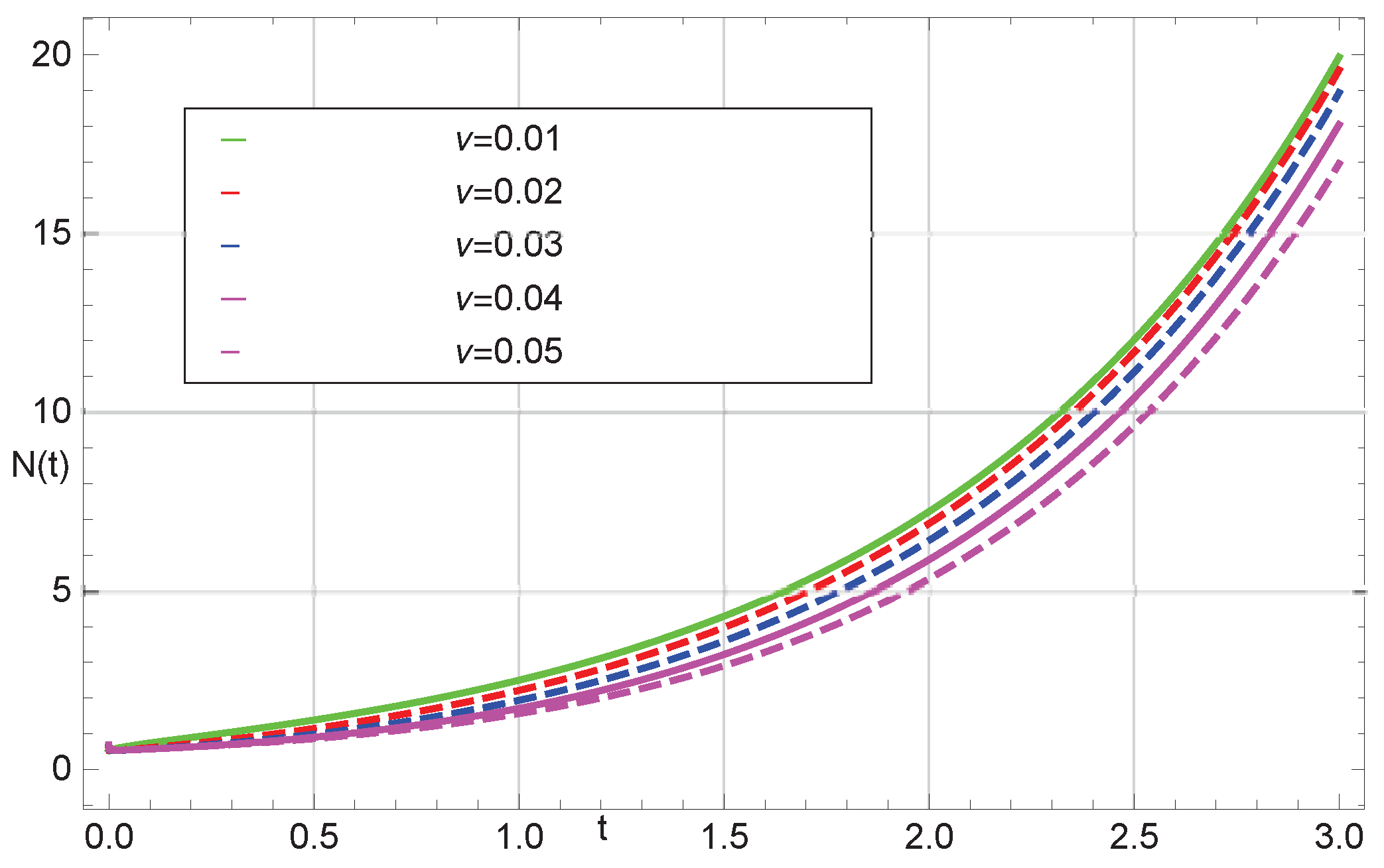
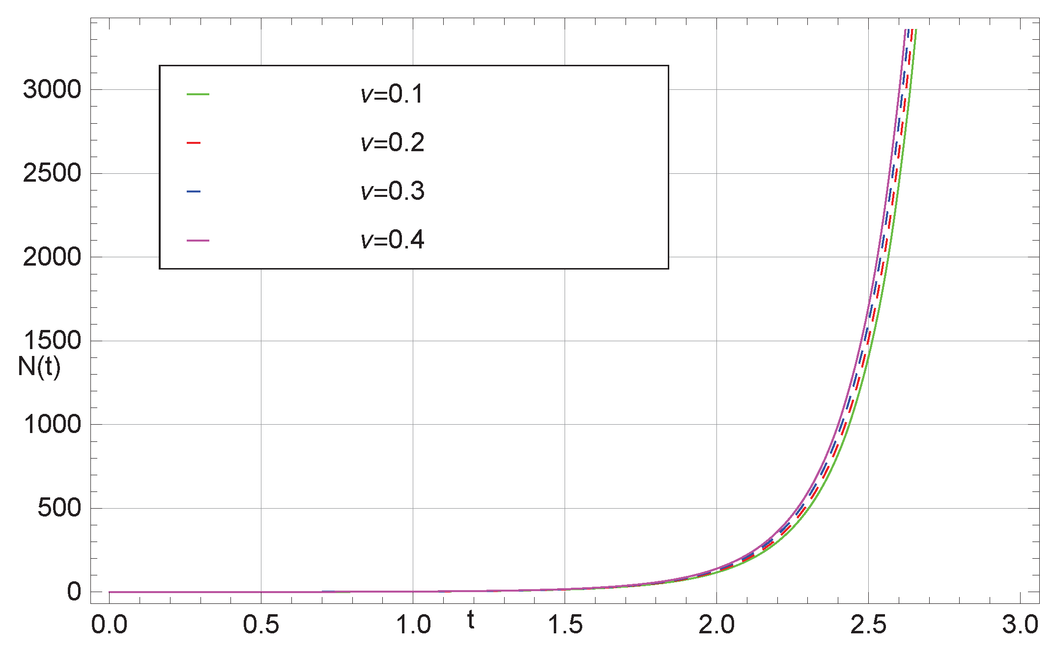
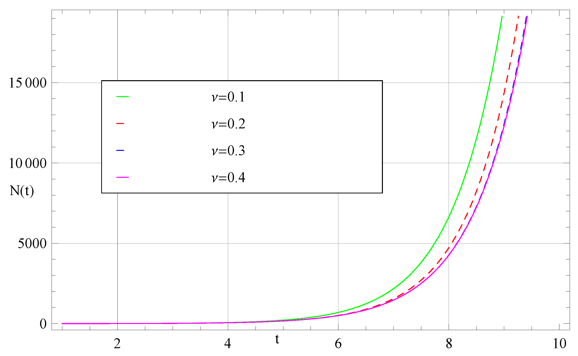
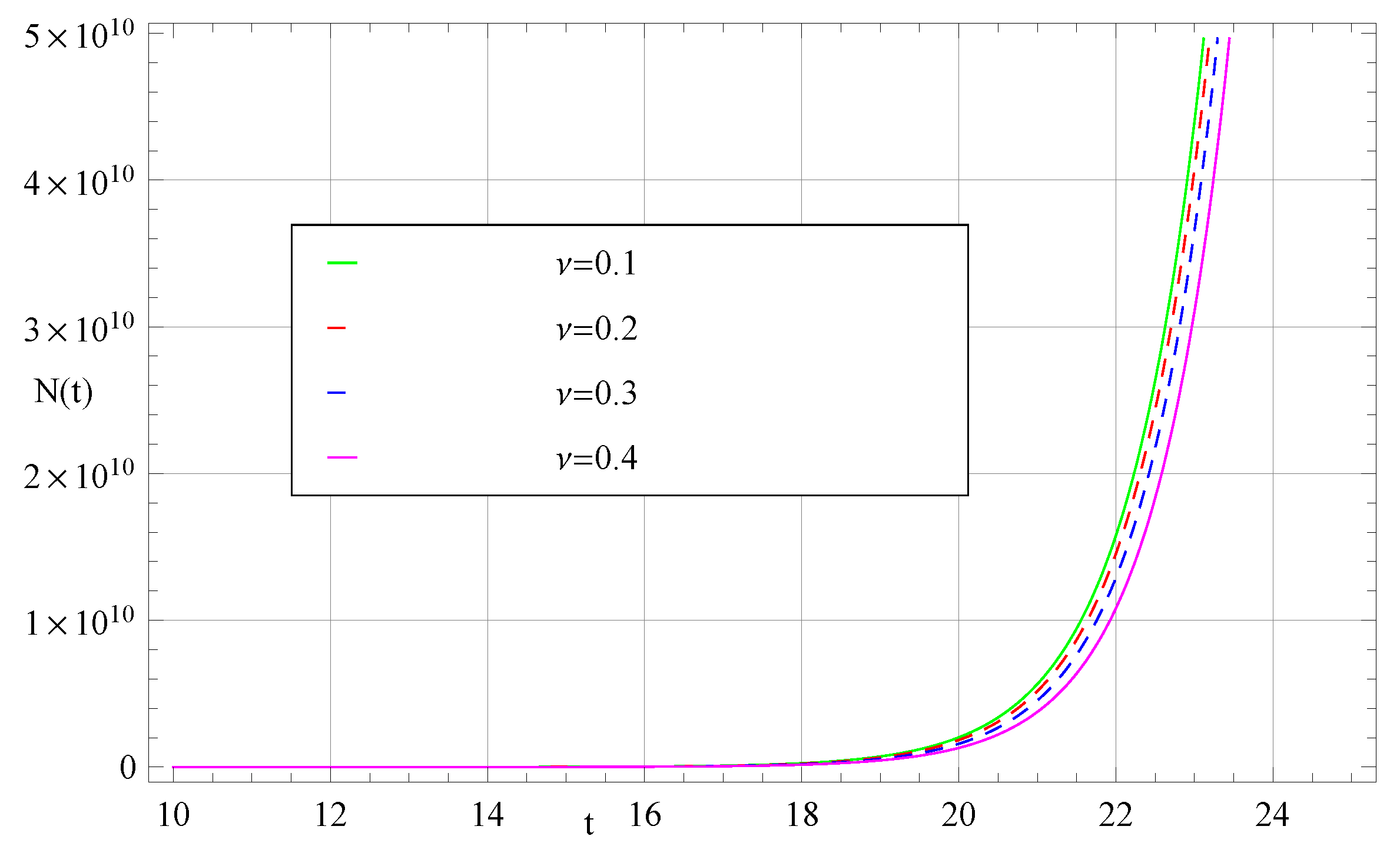
Figure 1 shows the plots of solutions of (31) with parametric values ${\mathfrak{N}}_{\mathfrak{0}}=1,d=1,\lambda =1,\mu =0.5$ and for different values of $\nu =0.01,0.02,0.03,0.04$, and $0.05$. The time interval $0<t<3$ gives the valid region of convergence of solutions. In Figure 2 the values of $\nu$ is considered as 0.1, 0.2, 0.3, and 0.4 for the same time interval. The Figure 3 and Figure 4 shows the 2D plots of solutions of (31) by considering the different time intervals. The graphical results demonstrate that the region of convergence of solutions depend continuously on the fractional parameter $\nu$. Hence, by examining the behavior of the solutions for different parameters and time interval it is observed that $\mathfrak{N}\left(t\right)$ is always positive.

6. Conclusions

The generalized Mittag-Leffler type function (GMLTF) is established and its fractional integral representations are studied in this paper. The obtained results are expressed in terms of the generalized Wright hypergeometric function. As an application of the function GMLTF given in this paper, the solutions of a fractional kinetic equation are studied using the Laplace transform technique. The results achieved here are rather general and found various new and known solutions of FKEs containing a different type of special function. The behavior of the obtained solutions is studied with the help of graphs. As a future direction, the generalized fractional calculus operators containing GMLTF can be studied and can be used to find the solutions of fractional kinetic or diffusion equations involving GMLTF with the help of different integral transform techniques.

References

- Srivastava, H.M.; Choi, J. Zeta and q-Zeta Functions and Associated Series and Integrals; Elsevier Science Publishers: Amsterdam, The Netherlands; London, UK; New York, NY, USA, 2012. [Google Scholar]
- Rainville, E.D. Special Functions; Macmillan: New York, NY, USA, 1960. [Google Scholar]
- Fox, C. The asymptotic expansion of generalized hypergeometric functions. Proc. Lond. Math. Soc. 1928, 27, 389–400. [Google Scholar] [CrossRef]
- Kilbas, A.A.; Saigo, M.; Trujillo, J.J. On the generalized Wright function. Fract. Calc. Appl. Anal. 2002, 5, 437–460. [Google Scholar]
- Wright, E.M. The asymptotic expansion of integral functions defined by Taylor series. Philos. Trans. R. Soc. Lond. Ser. A 1940, 238, 423–451. [Google Scholar] [CrossRef]
- Wright, E.M. The asymptotic expansion of the generalized hypergeometric function. Proc. Lond. Math. Soc. 1940, 46, 389–408. [Google Scholar] [CrossRef]
- Kilbas, A.A.; Srivastava, H.M.; Trujillo, J.J. Theory and Applications of Fractional Differential Equations; North-Holland Mathematics Studies 204; Elsevier: Amsterdam, The Netherlands, 2006. [Google Scholar]
- Kilbas, A.A.; Sebastian, N. Generalized fractional integration of Bessel function of the first kind. Int. Transf. Spec. Funct. 2008, 19, 869–883. [Google Scholar] [CrossRef]
- Thakar, U.; Joshi, V.; Vyawahare, V.A. Composite non-linear feedback control using Mittag-Leffler function. Int. J. Dyn. Control 2019, 7, 785–794. [Google Scholar] [CrossRef]
- Zhou, H.C.; Lv, C.; Guo, B.Z.; Chen, Y. Mittag-Leffler stabilization for an unstable time-fractional anomalous diffusion equation with boundary control matched disturbance. Int. J. Robust Nonlinear Control 2019, 29. [Google Scholar] [CrossRef]
- Kumar, D.; Baleanu, D. Fractional Calculus and its Applications in Physics. Front. Phys. 2019, 7, 81. [Google Scholar] [CrossRef]
- Djida, J.D.; Mophou, G.; Area, I. Optimal control of diffusion equation with fractional time derivative with nonlocal and nonsingular Mittag-Leffler kernel. J. Optim. Theory Appl. 2019, 182, 540–557. [Google Scholar] [CrossRef] [Green Version]
- Saqib, M.; Khan, I.; Shafie, S. New direction of Atangana–Baleanu fractional derivative with Mittag-Leffler kernel for non-Newtonian channel flow. In Fractional Derivatives with Mittag-Leffler Kernel; Springer: Cham, Switzerland, 2019; pp. 253–268. [Google Scholar]
- Bhatter, S.; Mathur, A.; Kumar, D.; Nisar, K.S.; Singh, J. Fractional modified Kawahara equation with Mittag–Leffler law. Chaos Solitons Fractals 2019, 2019, 109508. [Google Scholar] [CrossRef]
- Mittag-Leffler, G.M. Sur la representation analytiqie d’une fonction monogene cinquieme note. Acta Math. 1905, 29, 101–181. [Google Scholar] [CrossRef]
- Wiman, A. Uber den fundamental satz in der theorie der funktionen Eα (z). Acta Math. 1905, 29, 191–201. [Google Scholar] [CrossRef]
- Prabhakar, T.R. A singular integral equation with a generalized Mittag-Leffler function in the Kernel. Yokohama Math. J. 1971, 19, 7–15. [Google Scholar]
- Shukla, A.K.; Prajapati, J.C. On a generalization of Mittag-Leffler function and its properties. J. Math. Anal. Appl. 2007, 336, 797–811. [Google Scholar] [CrossRef] [Green Version]
- Salim, T.O. Some properties relating to the generalized Mittag-Leffler function. Adv. Appl. Math. Anal. 2009, 4, 21–30. [Google Scholar]
- Salim, T.O.; Faraj, A.W. A generalization of Mittag-Leffler function and integral operator associated with fractional calculus. J. Fract. Calc. Appl. 2012, 3, 1–13. [Google Scholar]
- Khan, M.A.; Ahmed, S. On some properties of the generalized Mittag-Leffler function. SpringerPlus 2013, 2, 337. [Google Scholar] [CrossRef] [Green Version]
- Sharma, K. Application of fractional calculus operators to related Areas. Gen. Math. Notes 2011, 7, 33–40. [Google Scholar]
- Srivastava, H.M.; Tomovski, Z. Fractional calculus with an integral operator containing a generalized Mittag–Leffler function in the kernel. Appl. Math. Comput. 2009, 211, 198–210. [Google Scholar] [CrossRef]
- Araci, S.; Rahman, G.; Ghaffar, A.; Nisar, K.S. Fractional Calculus of Extended Mittag-Leffler Function and Its Applications to Statistical Distribution. Mathematics 2019, 7, 248. [Google Scholar] [CrossRef] [Green Version]
- Andrić, M.; Farid, G.; Pećarić, J. A further extension of Mittag-Leffler function. Fract. Calc. Appl. Anal. 2018, 21, 1377–1395. [Google Scholar] [CrossRef]
- Bansal, M.K.; Jolly, N.; Jain, R.; Kumar, D. An integral operator involving generalized Mittag-Leffler function and associated fractional calculus results. J. Anal. 2019, 27, 727–740. [Google Scholar] [CrossRef]
- Choi, J.; Parmar, R.K.; Chopra, P. Extended Mittag-Leffler function and associated fractional calculus operators. Georgian Math. J. 2017. [Google Scholar] [CrossRef]
- Choi, J.; Rahman, G.; Nisar, K.S.; Mubeen, S.; Arshad, M. Formulas for Saigo fractional integral operators with 2F1 generalized k -Struve functions. Far East J. Math. Sci. 2017, 102, 55–66. [Google Scholar]
- Kumar, D.; Singh, J.; Baleanu, D. A new analysis of the Fornberg-Whitham equation pertaining to a fractional derivative with Mittag-Leffler-type kernel. Eur. Phys. J. Plus. 2018, 133, 70. [Google Scholar] [CrossRef]
- Parmar, R. A Class of Extended Mittag–Leffler Functions and Their Properties Related to Integral Transforms and Fractional Calculus. Mathematics 2015, 3, 1069–1082. [Google Scholar] [CrossRef] [Green Version]
- Rahman, G.; Baleanu, D.; Qurashi, M.A.; Purohit, S.D.; Mubeen, S.; Arshad, M. The extended Mittag-Leffler function via fractional calculus. J. Nonlinear Sci. Appl. 2017, 10, 4244–4253. [Google Scholar] [CrossRef]
- Rahman, G.; Nisar, K.S.; Choi, J.; Mubeen, S.; Arshad, M. Pathway Fractional Integral Formulas Involving Extended Mittag-Leffler Functions in the Kernel. Kyungpook Math. J. 2019, 59, 125–134. [Google Scholar]
- Choi, J.; Rahman, G.; Mubeen, S.; Nisar, K.S. Certain extended special functions and fractional integral and derivative operators via an extended beta function. Nonlinear Funct. Anal. Appl. 2019, 24, 1–13. [Google Scholar]
- Shang, Y. Vulnerability of networks: Fractional percolation on random graphs. Phys. Rev. E 2014, 89, 012813. [Google Scholar] [CrossRef]
- Kiryakova, V. All the special functions are fractional differintegrals of elementary functions. J. Phys. A 1977, 30, 5085–5103. [Google Scholar] [CrossRef] [Green Version]
- Machado, J.T. Fractional derivatives and negative probabilities. Commun. Nonlinear Sci. Numer. Simul. 2019, 79, 104913. [Google Scholar] [CrossRef]
- Machado, J.T. Fractional calculus: Fundamentals and applications. In Acoustics and Vibration of Mechanical Structures—AVMS-2017, Proceedings of the 14th AVMS Conference, Timisoara, Romania, 25–26 May 2017; Springer: Cham, Switzerland, 2018; pp. 3–11. [Google Scholar]
- Machado, J.T.; Kiryakova, V.; Mainardi, F. Recent history of fractional calculus. Commun. Nonlinear Sci. Numer. Simul. 2011, 16, 1140–1153. [Google Scholar] [CrossRef] [Green Version]
- Machado, J.T.; Galhano, A.M.; Trujillo, J.J. On development of fractional calculus during the last fifty years. Scientometrics 2014, 98, 577–582. [Google Scholar] [CrossRef] [Green Version]
- Miller, K.S.; Ross, B. An Introduction to the Fractional Calculus and Fractional Differential Equations; Wiley: New York, NY, USA, 1993. [Google Scholar]
- Srivastava, H.M.; Lin, S.-D.; Wang, P.-Y. Some fractional-calculus results for the H-function associated with a class of Feynman integrals. Russ. J. Math. Phys. 2006, 13, 94–100. [Google Scholar] [CrossRef]
- Haubold, H.J.; Mathai, A.M. The fractional kinetic equation and thermonuclear functions. Astrophys. Space Sci. 2000, 327, 53–63. [Google Scholar] [CrossRef]
- Saxena, R.K.; Mathai, A.M.; Haubold, H.J. On Fractional kinetic equations. Astrophys. Space Sci. 2002, 282, 281–287. [Google Scholar] [CrossRef] [Green Version]
- Saxena, R.K.; Mathai, A.M.; Haubold, H.J. On generalized fractional kinetic equations. Physica A 2004, 344, 657–664. [Google Scholar] [CrossRef] [Green Version]
- Saxena, R.K.; Mathai, A.M.; Haubold, H.J. Solution of generalized fractional reaction-diffusion equations. Astrophys. Space Sci. 2006, 305, 305–313. [Google Scholar] [CrossRef] [Green Version]
- Saxena, R.K.; Kalla, S.L. On the solutions of certain fractional kinetic equations. Appl. Math. Comput. 2008, 199, 504–511. [Google Scholar] [CrossRef]
- Saichev, A.; Zaslavsky, M. Fractional kinetic equations: Solutions and applications. Chaos 1997, 7, 753–764. [Google Scholar] [CrossRef] [PubMed] [Green Version]
- Gupta, V.G.; Sharma, B.; Belgacem, F.B.M. On the solutions of generalized fractional kinetic equations. Appl. Math. Sci. 2011, 5, 899–910. [Google Scholar] [CrossRef] [Green Version]
- Gupta, A.; Parihar, C.L. On solutions of generalized kinetic equations of fractional order. Bol. Soc. Paran. Mat. 2014, 32, 181–189. [Google Scholar] [CrossRef] [Green Version]
- Nisar, K.S.; Purohit, S.D.; Mondal, S.R. Generalized fractional kinetic equations involving generalized Struve function of the first kind. J. King Saud Univ. -Sci. 2016, 28, 167–171. [Google Scholar] [CrossRef] [Green Version]
- Erdélyi, A.; Magnus, W.; Oberhettinger, F.; Tricomi, F.G. Tables of Integral Transforms; Based, in part, on notes left by Harry Bateman; McGraw-Hill Book Company, Inc.: New York, NY, USA; Toronto, ON, Canada; London, UK, 1954; Volume II. [Google Scholar]
- Srivastava, H.M.; Saxena, R.K. Operators of fractional integration and their applications. Appl. Math. Comput. 2001, 118, 1–52. [Google Scholar] [CrossRef]
- Shang, Y. Localized recovery of complex networks against failure. Sci. Rep. 2016, 6, 30521. [Google Scholar] [CrossRef] [Green Version]
- Shang, Y. Percolation on random networks with proliferation. Int. J. Mod. Phys. B 2018, 32, 1850359. [Google Scholar] [CrossRef]
Figure 1.
Graph of the solution (31).
Figure 2.
Figure 3.
Figure 4.
© 2019 by the author. Licensee MDPI, Basel, Switzerland. This article is an open access article distributed under the terms and conditions of the Creative Commons Attribution (CC BY) license (http://creativecommons.org/licenses/by/4.0/).
Share and Cite
MDPI and ACS Style
Nisar, K.S. Fractional Integrations of a Generalized Mittag-Leffler Type Function and Its Application. Mathematics 2019, 7, 1230. https://doi.org/10.3390/math7121230
AMA Style
Nisar KS. Fractional Integrations of a Generalized Mittag-Leffler Type Function and Its Application. Mathematics. 2019; 7(12):1230. https://doi.org/10.3390/math7121230
Chicago/Turabian StyleNisar, Kottakkaran Sooppy. 2019. "Fractional Integrations of a Generalized Mittag-Leffler Type Function and Its Application" Mathematics 7, no. 12: 1230. https://doi.org/10.3390/math7121230
Note that from the first issue of 2016, this journal uses article numbers instead of page numbers. See further details here.