An Efficient Local Formulation for Time–Dependent PDEs

Abstract

In this paper, a local meshless method (LMM) based on radial basis functions (RBFs) is utilized for the numerical solution of various types of PDEs. This local approach has flexibility with respect to geometry along with high order of convergence rate. In case of global meshless methods, the two major deficiencies are the computational cost and the optimum value of shape parameter. Therefore, research is currently focused towards localized RBFs approximations, as proposed here. The proposed local meshless procedure is used for spatial discretization, whereas for temporal discretization, different time integrators are employed. The proposed local meshless method is testified in terms of efficiency, accuracy and ease of implementation on regular and irregular domains.

1. Introduction

Partial differential equation (PDE) of reaction-convection-diffusion type are physically very rich. These PDEs can be abundantly found in modeling physical sciences, biological sciences and mathematics of finance. Some of these models include the fifth order Kortewege-de Vries model. Its general exact solution is not known whereas the exact solution for particular case of solitary waves can be found in [1]. To solve this model numerically, serval methods can be found in literature such as finite-deference scheme [2], modified ADM [3], decomposition method [4], Homotopy perturbation transform method [5] and a comparative study of Crank-Nicolson method and ADM [6].

The general seventh order Kortewege-de Vries equation [7] which is used to discuss structural stability under singular perturbation of standard KdV equation. Several authors have paid attention to solve the seventh order KdV equation [8,9,10].

Generalized Burgers’ Huxley equation [11] is used to describe the interaction between convection effects, reaction mechanisms and diffusion transports. In general it is difficult and sometimes impossible to get exact solution of such type of nonlinear PDEs. Researchers employed different numerical techniques which include discrete Adomian decomposition method [12], Haar wavelet method [13], Adomian decomposition method [14], meshless collocation method based on RBF [15] and local meshless method [16] for the solution of Burgers’ Huxley equation. The Huxley model equation [17] describes nerve pulse propagation in nerve fibres and wall motion in liquid crystals [18]. Numerical solution of Huxley equation can be found in [14,15,19] and the references therein. Generalized Burgers’ Fisher equation [20], describe the propagation of a mutant gene. Different numerical methods have been used for numerical solution of this model, such as meshless collocation method [15], ADM [14], VIM [21], modified pseudo spectral method [22] and modified cubic B–spline functions collocation method [23].

The Fitzhugh-Nagumo (FN) equation has numerous applications in different fields such as branching brownian motion process, flame propagation, neurophysiology, logistic population growth and nuclear reactor theory [24]. Numerical solution of FN equation can be found in [23,25,26,27].

Hirota-Satsuma introduced the nonlinear coupled Kortewege-de Vries equations [28]. This model has numerous applications in physical sciences. In the last decade, researchers have used various numerical techniques for the solution of this model equations. These include RBFs collocation (Kansa) method [29], meshless RBFs method of lines [30], variational iteration method [31] and spectral collocation method [32]. The Hirota–Satsuma coupled KdV system [33] has been solved by different numerical methods given in [32,34,35] and the references therein.

The Brusselator system is one of the essential reaction–diffusion model equation. This model explain the mechanism of a chemical reaction–diffusion with non–linear oscillations [36,37]. Numerical solution of this kind of model can be found in [38,39,40,41].

The horizon of meshless methods is continuously expanding and their applicability is increasing rapidly due to their ease of implementation in higher dimensions on a set of uniform or scattered data points in regular and irregular geometries. In the last few years, it is observed that meshless methods have been extensively employed for numerical simulations of different types of PDEs [29,42,43,44]. Meshless methods reduce complexity caused due to dimensionality to a large extent which is being faced in the carrying out of conventional methods like finite-element and finite-difference procedures. Meshing in the case of complicated geometries is another cause for the growing demand of meshless methods.

It is noticed that the global meshless method (GMM) which is based on global interpolation paradigm faced the problem of dense ill-conditioned matrices and finding optimum value of the shape parameter. To avoid limitations of the GMM, a local meshless method which is based on local interpolation in the sub-domains are used as substitute to get a stable and accurate solution for the PDE models [43,45,46,47,48].

Organization of rest of the paper is as follows; In Section 2, we describe the models briefly. In Section 3, we highlight the proposed method. In Section 4, the numerical methods are applied to different test problems and the results are compared with published work. In Section 5, some conclusions are drawn.

2. Partial Differential Equation Models

A short description of PDE models on a bounded domain with corresponding initial and boundary conditions are given in this section. These include; one-dimensional fifth order Lax’s- Kortewege-de Vries, seventh order Lax’s-Kortewege-de Vries, generalized Burgers’-Huxley, Huxley, generalized Burgers’ Fisher, Fitzhugh-Nagumo, coupled Kortewege-de Vries, Hirota-Satsuma coupled Kortewege-de Vries equations and two-dimensional reaction-diffusion Brusselator equations.

The 1D fifth order Kortewege-de Vries equation [3],

$$U_t+a{U}^2{U}_x+b{U}_x{U}_{xx}+cU{U}_{xxx}+d{U}_{xxxxx}=0,$$

(1)

where a, b, c, d are real constants and in this paper we have taken $a=b=30$, $c=10$, and $d=1$.

The 1D seventh order Kortewege-de Vries equation [9],

$$U_t+a{U}^3{U}_x+b{U}_x^3+cU{U}_x{U}_{xx}+d{U}^2{U}_{xxx}+e{U}_{xx}{U}_{xxx}+f{U}_x{U}_{xxxx}+gU{U}_{xxxxx}+U_{xxxxxxx}=0,$$

(2)

where a, b, c, d, e, f, g are real constants and we have taken $a=140$, $b=70$, $c=280$, $d=70$, $e=70$, $f=42$, $g=14$.

The 1D generalized Burgers’-Huxley equation [11,12,13,14,15],

$$U_t+\alpha U^{\delta }{U}_x-U_{xx}-\beta U(1-U^{\delta })(U^{\delta }-\gamma )=0,$$

(3)

where $\alpha$, $\beta \ge 0$, $\delta >0$, $\gamma \in (0,1)$ are constants.

The 1D Huxley equation [14,15,19],

$$U_t-U_{xx}-\beta U(1-U)(U-\gamma )=0,$$

(4)

where $\beta$ and $\gamma$ are constants.

The 1D generalized Burgers’ Fisher equation [14,15],

$$U_t+\alpha U^{\delta }{U}_x-U_{xx}-\beta U(1-U^{\delta })=0,$$

(5)

where $\alpha$, $\beta$ and $\delta$ are constants.

The 1D Fitzhugh-Nagumo (FN) equation [24,27,49,50],

$$U_t-U_{xx}+U(1-U)(\rho -U)=0,$$

(6)

where $\rho$ is a constant.

The 1D coupled Kortewege-de Vries equation [28,29,30,32],

$$\begin{array}{r}{U}_t+6\alpha U{U}_x-2\gamma V{V}_x+\alpha U_{xxx}=0,\\ V_t+3\beta U{V}_x+\beta V_{xxx}=0,\end{array}$$

(7)

where $\alpha$, $\beta$ and $\gamma$ are real parameters.

The 1D Hirota-Satsuma coupled KdV system of equations [32,33],

$$\begin{array}{rr}{U}_t-\frac{1}{2}{U}_{xxx}+3U{U}_x-3V{W}_x-3W{V}_x& =0,\\ V_t+V_{xxx}-3U{V}_x& =0,\\ W_t+W_{xxx}-3U{W}_x& =0.\end{array}$$

(8)

The 2D reaction-diffusion Brusselator system of equations [38,41],

$$\begin{array}{r}{U}_t-\beta -U^{2}V+(\alpha +1)U-\gamma (U_{xx}+U_{yy})=0,\\ V_t-\alpha U+U^{2}V-\gamma (V_{xx}+V_{yy})=0,\end{array}$$

(9)

where $\alpha$, $\beta$ and $\gamma$ are constants.

3. Local Meshless Numerical Scheme

To pursue the LMM [43,51], we approximate the derivatives of $U(x,t)$ at the center $x_p$ by the function values at a set of nodes in the neighborhood of $x_p$, $\{x_{p_1},x_{p_2},x_{p_3},\dots ,x_{p_{n_j}}\}\subset \{x_1,x_2,\dots ,x_{N^n}\},n_p\ll N^n$, where $n=1$, $n=2$ for one and two dimensional case respectively.

$$U^{\left(m\right)}\left(x_p\right)\approx {\displaystyle \sum _{k=1}^{n_p}}{\lambda }_k^{\left(m\right)}U\left(x_{p_k}\right),p=1,2,\dots ,N^n.$$

(10)

To find the corresponding coefficient ${\lambda }_k^{\left(m\right)}$, radial basis function $\varphi (\parallel x-x_l\parallel )$ can be substituted into Equation (10)

$${\varphi }^{\left(m\right)}(\parallel x_p-x_l\parallel )={\displaystyle \sum _{k=1}^{n_p}}{\lambda }_{p_k}^{\left(m\right)}\varphi (\parallel x_{p_k}-x_l\parallel ),l=p_1,p_2,\dots ,p_{n_p}.$$

(11)

Equation (11) in matrix form

$$\left[\begin{array}{c}{\varphi }_{p_1}^{\left(m\right)}\left(x_p\right)\\ {\varphi }_{p_2}^{\left(m\right)}\left(x_p\right)\\ ⋮\\ {\varphi }_{p_{n_p}}^{\left(m\right)}\left(x_p\right)\end{array}\right]=\left[\begin{array}{cccc}{\varphi }_{p_1}\left(x_{p_1}\right)& {\varphi }_{p_2}\left(x_{p_1}\right)& \cdots & {\varphi }_{p_{n_p}}\left(x_{p_1}\right)\\ {\varphi }_{p_1}\left(x_{p_2}\right)& {\varphi }_{p_2}\left(x_{p_2}\right)& \cdots & {\varphi }_{p_{n_p}}\left(x_{p_2}\right)\\ ⋮& ⋮& \ddots & ⋮\\ {\varphi }_{p_1}\left(x_{p_{n_p}}\right)& {\varphi }_{p_2}\left(x_{p_{n_p}}\right)& \cdots & {\varphi }_{p_{n_p}}\left(x_{p_{n_p}}\right)\end{array}\right]\left[\begin{array}{c}{\lambda }_{p_1}^{\left(m\right)}\\ {\lambda }_{p_2}^{\left(m\right)}\\ ⋮\\ {\lambda }_{p_{n_p}}^{\left(m\right)}\end{array}\right],$$

(12)

where

$${\varphi }_l\left(x_k\right)=\varphi (\parallel x_k-x_l\parallel ),l=p_1,p_2,\dots ,p_{n_p},$$

(13)

for each $k=p_1,p_2,\dots ,p_{n_p}$.

The above equation in matrix notation

$${\mathbf{\Phi }}_{n_p}^{\left(m\right)}={\mathbf{A}}_{n_p}{\mathit{\lambda }}_{n_p}^{\left(m\right)},$$

(14)

where

$${\mathbf{\Phi }}_{n_p}^{\left(m\right)}={\left[\begin{array}{cccc}{\varphi }_{p_1}^{\left(m\right)}\left(x_p\right)& {\varphi }_{p_2}^{\left(m\right)}\left(x_p\right)& \cdots & {\varphi }_{p_{n_p}}^{\left(m\right)}\left(x_p\right)\end{array}\right]}^T$$

$${\mathbf{A}}_{n_p}=\left[\begin{array}{cccc}{\varphi }_{p_1}\left(x_{p_1}\right)& {\varphi }_{p_2}\left(x_{p_1}\right)& \cdots & {\varphi }_{p_{n_p}}\left(x_{p_1}\right)\\ {\varphi }_{p_1}\left(x_{p_2}\right)& {\varphi }_{p_2}\left(x_{p_2}\right)& \cdots & {\varphi }_{p_{n_p}}\left(x_{p_2}\right)\\ ⋮& ⋮& \ddots & ⋮\\ {\varphi }_{p_1}\left(x_{p_{n_p}}\right)& {\varphi }_{p_2}\left(x_{p_{n_p}}\right)& \cdots & {\varphi }_{p_{n_p}}\left(x_{p_{n_p}}\right)\end{array}\right]$$

$${\mathit{\lambda }}_{n_p}^{\left(m\right)}={\left[\begin{array}{cccc}{\lambda }_{p_1}^{\left(m\right)}& {\lambda }_{p_2}^{\left(m\right)}& \cdots & {\lambda }_{p_{n_p}}^{\left(m\right)}\end{array}\right]}^T.$$

From Equation (14),

$${\mathit{\lambda }}_{n_p}^{\left(m\right)}={\mathbf{A}}_{n_p}^{-1}{\mathbf{\Phi }}_{n_p}^{\left(m\right)}.$$

(15)

By substituting Equation (15) into Equation (10),

$$U^{\left(m\right)}\left(x_p\right)={\left({\mathit{\lambda }}_{n_p}^{\left(m\right)}\right)}^T{\mathbf{U}}_{n_p},$$

(16)

where

$${\mathbf{U}}_{n_p}={\left[U\left(x_{p_1}\right),U\left(x_{p_2}\right),\dots ,U\left(x_{p_{n_p}}\right)\right]}^T.$$

(17)

3.1. 1D Fifth Order Kortewege-de Vries Equation

The 1D fifth order Kortewege-de Vries Equation (1) can be written as

$$U_t=-(a{U}^2{U}_x+b{U}_x{U}_{xx}+cU{U}_{xxx}+d{U}_{xxxxx}),x\in \Omega ,t\ge 0,$$

(18)

subject to initial and boundary conditions

$$U(x,0)=f\left(x\right),x\in \Omega ,$$

(19)

$$U(x,t)=f_1\left(t\right),U(x,t)=f_2\left(t\right),x\in \partial \Omega .$$

(20)

where a, b, c and d are constants.

Now, Applying the LMM to Equation (18) we get,

$$\frac{d{U}_p}{dt}=-(a{U}_p^2{\left({\mathit{\lambda }}_{n_p}^{\left(1\right)}\right)}^T{\mathbf{U}}_{n_p}+b\left({\left({\mathit{\lambda }}_{n_p}^{\left(1\right)}\right)}^T{\mathbf{U}}_{n_p}\right)\left({\left({\mathit{\lambda }}_{n_p}^{\left(2\right)}\right)}^T{\mathbf{U}}_{n_p}\right)+c{U}_p{\left({\mathit{\lambda }}_{n_p}^{\left(3\right)}\right)}^T{\mathbf{U}}_{n_p}+d{\left({\mathit{\lambda }}_{n_p}^{\left(5\right)}\right)}^T{\mathbf{U}}_{n_p}),p=2,3,\dots ,N-1.$$

(21)

The semi-discretized model Equation (21) with boundary conditions (20) is given as follows

$$\frac{d\mathfrak{U}}{dt}=-(a{\mathfrak{U}}^2\ast \left({\mathbf{\Lambda }}^{\left(1\right)}\mathfrak{U}\right)+b\left({\mathbf{\Lambda }}^{\left(1\right)}\mathfrak{U}\right)\ast \left({\mathbf{\Lambda }}^{\left(2\right)}\mathfrak{U}\right)+c\mathfrak{U}\ast \left({\mathbf{\Lambda }}^{\left(3\right)}\mathfrak{U}\right)+d\left({\mathbf{\Lambda }}^{\left(5\right)}\mathfrak{U}\right)),$$

(22)

where the symbol * represent element-wise multiplication of two vectors.

$$\begin{array}{cc}\hfill \mathfrak{U}& ={[U_1,U_2,U_3,\dots ,U_N]}^T,\hfill \\ \hfill {\mathbf{\Lambda }}_{N\times N}^{\left(1\right)}& =\left[m_{pk}\right]=\left[{\mathit{\lambda }}_k^{\left(1\right)}\right],k=p_1,p_2,\dots ,p_{n_p},p=2,3,\dots ,N-1,\hfill \\ \hfill {\mathbf{\Lambda }}_{N\times N}^{\left(2\right)}& =\left[m_{pk}\right]=\left[{\mathit{\lambda }}_k^{\left(2\right)}\right],k=p_1,p_2,\dots ,p_{n_p},p=2,3,\dots ,N-1.\hfill \\ \hfill {\mathbf{\Lambda }}_{N\times N}^{\left(3\right)}& =\left[m_{pk}\right]=\left[{\mathit{\lambda }}_k^{\left(3\right)}\right],k=p_1,p_2,\dots ,p_{n_p},p=2,3,\dots ,N-1.\hfill \\ \hfill {\mathbf{\Lambda }}_{N\times N}^{\left(5\right)}& =\left[m_{pk}\right]=\left[{\mathit{\lambda }}_k^{\left(5\right)}\right],k=p_1,p_2,\dots ,p_{n_p},p=2,3,\dots ,N-1.\hfill \end{array}$$

(23)

The corresponding initial condition is given as

$$\mathfrak{U}\left(t_0\right)={[U_0\left(x_1\right),U_0\left(x_2\right),\dots ,U_0\left(x_N\right)]}^T.$$

(24)

4. Results and Discussion

To check the accuracy and efficiency of the LMM various test problems in one and two dimensional cases are considered and the results are compared with the existence methods reported in literature. For spatial discretization three types of RBFs that is, multiquadric (MQ), inverse multiquadric (IMQ) and Gaussian (GA) are used whereas for time integration have used explicit Euler method (EEM) and Runge-Kutta method of order 4 (RK4).

Accuracy of the LMM is measured though different error norms given as follows

$$\begin{array}{cc}\hfill L_{abs}& =|U_{exact}\left(p\right)-U\left(p\right)|,p=1,2,\dots ,N^n.\hfill \\ \hfill L_{\infty }& =\max \left(|U_{exact}\left(p\right)-U\left(p\right)|\right),\hfill \\ \hfill L_2& ={\left[\Delta x{\displaystyle \sum _{p=1}^N}{L_{abs}}^2\right]}^{\frac{1}{2}},\hfill \\ \hfill L_{rms}& ={\left[\frac{1}{N}{\displaystyle \sum _{p=1}^N}{L_{abs}}^2\right]}^{\frac{1}{2}},\hfill \end{array}$$

(25)

where exact and numerical solution are represented by $U_{exact}$ and U respectively.

In this paper, we have considered both uniform and non-uniform nodal points. In 1D case, the size of local sub domain is taken $n_p=3$ whereas in 2D case the size of the local sub domain is taken $n_p=5$ for all the numerical experiments. The Central Processing Unit (CPU) time is calculated in seconds in all the cases.

Summary of numerical results is given as: Results of 1D fifth order KdV equation are shown in

Table 1. Comparisons between the results obtained by the LMM with those adapted from [3] for Test Problem 1.

	x = 0.2		x = 1		x = 5
$\mathit{t}$	EEM	[3]	EEM	[3]	EEM	[3]
2	5.2899 × ${10}^{-15}$	5.7619 × ${10}^{-14}$	2.6450 × ${10}^{-14}$	2.8786 × ${10}^{-13}$	1.2669 × ${10}^{-13}$	1.4210 × ${10}^{-12}$
4	1.0580 × ${10}^{-14}$	1.1528 × ${10}^{-13}$	5.2900 × ${10}^{-14}$	5.7577 × ${10}^{-13}$	2.5337 × ${10}^{-13}$	2.8421 × ${10}^{-12}$
6	1.5869 × ${10}^{-14}$	1.7298 × ${10}^{-13}$	7.9350 × ${10}^{-14}$	8.6372 × ${10}^{-13}$	3.8006 × ${10}^{-13}$	4.2632 × ${10}^{-12}$
8	2.1159 × ${10}^{-14}$	2.3073 × ${10}^{-13}$	1.0580 × ${10}^{-13}$	1.1517 × ${10}^{-12}$	5.0676 × ${10}^{-13}$	5.6844 × ${10}^{-12}$
10	2.6448 × ${10}^{-14}$	2.8851 × ${10}^{-13}$	1.3225 × ${10}^{-13}$	1.4397 × ${10}^{-12}$	6.3345 × ${10}^{-13}$	7.1056 × ${10}^{-12}$

and compared with the method in [3] whereas numerical results of seventh order KdV equation are presented in

Table 2. Numerical results in form of $L_{\infty }$ error norm using the EEM for Test Problem 2.

t	k = 0.1	k = 0.01	k = 0.001	CPU Time
1	5.8157 × ${10}^{-10}$	1.2395 × ${10}^{-15}$	3.3881 × ${10}^{-19}$	0.03
10	5.8205 × ${10}^{-9}$	1.2395 × ${10}^{-14}$	3.3881 × ${10}^{-18}$	0.21
20	1.1652 × ${10}^{-8}$	2.4790 × ${10}^{-14}$	6.7763 × ${10}^{-18}$	0.46
30	1.7494 × ${10}^{-8}$	3.7185 × ${10}^{-14}$	1.0164 × ${10}^{-17}$	0.71
50	2.9211 × ${10}^{-8}$	6.1975 × ${10}^{-14}$	1.6941 × ${10}^{-17}$	1.07

. Similarly the numerical results of generalized Burgers’ Huxley equation are presented in

Table 3. Comparisons between the results obtained by the LMM with those adapted from [12,14,15] in term of $L_{abs}$ error norm for Test Problem 3.

t	x	RK4	[15]	[14]	[12]
0.05	0.1	6.30 × ${10}^{-12}$	1.0 × ${10}^{-9}$	1.93 × ${10}^{-7}$	1.87 × ${10}^{-8}$
	0.5	4.42 × ${10}^{-12}$	1.0 × ${10}^{-9}$	1.93 × ${10}^{-7}$	1.87 × ${10}^{-8}$
	0.9	2.55 × ${10}^{-12}$	1.0 × ${10}^{-9}$	1.93 × ${10}^{-7}$	1.87 × ${10}^{-8}$
0.1	0.1	1.23 × ${10}^{-11}$	1.0 × ${10}^{-9}$	3.87 × ${10}^{-7}$	3.75 × ${10}^{-8}$
	0.5	8.62 × ${10}^{-12}$	1.0 × ${10}^{-9}$	3.87 × ${10}^{-7}$	3.75 × ${10}^{-8}$
	0.9	4.87 × ${10}^{-12}$	1.0 × ${10}^{-9}$	3.87 × ${10}^{-7}$	3.75 × ${10}^{-8}$
1.0	0.1	8.16 × ${10}^{-11}$	0.0 × ${10}^{-9}$	3.88 × ${10}^{-6}$	3.75 × ${10}^{-7}$
	0.5	4.41 × ${10}^{-11}$	0.0 × ${10}^{-9}$	3.88 × ${10}^{-6}$	3.75 × ${10}^{-7}$
	0.9	6.61 × ${10}^{-12}$	0.0 × ${10}^{-9}$	3.88 × ${10}^{-6}$	3.75 × ${10}^{-7}$

and

Table 4. Comparisons between the results obtained by the LMM with those adapted from [13] in term of $L_{abs}$ error norm for Test Problem 3.

	$\mathit{\delta }\mathbf{=}\mathbf{1}$	$\mathit{\delta }\mathbf{=}\mathbf{1}$	$\mathit{\delta }\mathbf{=}\mathbf{2}$	$\mathit{\delta }\mathbf{=}\mathbf{2}$
x	RK4	[13]	RK4	[13]
0.15625	6.8575 × ${10}^{-11}$	2.4648 × ${10}^{-8}$	5.9052 × ${10}^{-7}$	1.1465 × ${10}^{-6}$
0.28125	5.9200 × ${10}^{-11}$	3.7832 × ${10}^{-8}$	5.8977 × ${10}^{-7}$	1.7600 × ${10}^{-6}$
0.34375	5.4512 × ${10}^{-11}$	4.2226 × ${10}^{-8}$	5.8940 × ${10}^{-7}$	1.9644 × ${10}^{-6}$
0.46875	4.5137 × ${10}^{-11}$	4.6621 × ${10}^{-8}$	5.8866 × ${10}^{-7}$	2.1749 × ${10}^{-6}$
0.53125	4.0448 × ${10}^{-11}$	4.6622 × ${10}^{-8}$	5.8828 × ${10}^{-7}$	2.1749 × ${10}^{-6}$
0.65625	3.1070 × ${10}^{-11}$	4.2228 × ${10}^{-8}$	5.8754 × ${10}^{-7}$	1.9643 × ${10}^{-6}$
0.71875	2.6382 × ${10}^{-11}$	3.7834 × ${10}^{-8}$	5.8717 × ${10}^{-7}$	1.7603 × ${10}^{-6}$
0.84375	1.7004 × ${10}^{-11}$	2.4650 × ${10}^{-8}$	5.8642 × ${10}^{-7}$	1.1462 × ${10}^{-6}$
0.96875	7.6260 × ${10}^{-12}$	5.5962 × ${10}^{-9}$	5.8568 × ${10}^{-7}$	2.6037 × ${10}^{-7}$

and the results are compared with the methods given in [12,13,14,15] while the numerical results of Huxley equation are shown in

Table 5. Comparisons between the results obtained by the LMM with those adapted from [14,15] in term of $L_{abs}$ error norm for Test Problem 3.

t	x	RK4	[15]	[14]
	0.1	2.18 × ${10}^{-11}$	0.0 × ${10}^{-9}$	1.88 × ${10}^{-7}$
0.05	0.5	1.83 × ${10}^{-11}$	1.0 × ${10}^{-9}$	1.87 × ${10}^{-7}$
	0.9	1.47 × ${10}^{-11}$	1.0 × ${10}^{-9}$	1.87 × ${10}^{-7}$
	0.1	4.29 × ${10}^{-11}$	1.0 × ${10}^{-9}$	3.75 × ${10}^{-7}$
0.1	0.5	3.59 × ${10}^{-11}$	0.0 × ${10}^{-9}$	3.75 × ${10}^{-7}$
	0.9	2.88 × ${10}^{-11}$	0.0 × ${10}^{-9}$	3.75 × ${10}^{-7}$
	0.1	3.18 × ${10}^{-10}$	1.0 × ${10}^{-9}$	3.75 × ${10}^{-6}$
1.0	0.5	2.47 × ${10}^{-10}$	0.0 × ${10}^{-9}$	3.75 × ${10}^{-6}$
	0.9	1.76 × ${10}^{-10}$	1.0 × ${10}^{-9}$	3.75 × ${10}^{-6}$

and

Table 6. Comparisons between the results obtained by the LMM with those adapted from [19] in term of $L_{abs}$ error norm for Test Problem 4.

a	b	t	x	EEM	[19]
−2	2	0.002	0.050	1.9974 × ${10}^{-7}$	2.22 × ${10}^{-3}$
−2	2	0.100	0.700	3.0067 × ${10}^{-6}$	1.78 × ${10}^{-3}$
−5	5	0.001	0.500	2.5260 × ${10}^{-7}$	1.69 × ${10}^{-2}$
−5	5	0.001	2.500	1.7843 × ${10}^{-6}$	9.90 × ${10}^{-3}$
−10	10	0.002	0.010	3.6673 × ${10}^{-6}$	4.05 × ${10}^{-4}$
−10	10	0.100	1.000	2.7722 × ${10}^{-4}$	3.17 × ${10}^{-3}$

and compared with the methods in [14,15,19]. Numerical results of generalized Burgers’ Fisher equation are shown in

Table 7. Comparisons between the results obtained by the LMM with those adapted from [14,15] in term of $L_{abs}$ error norm for Test Problem 5.

t	x	RK4	[15]	[14]
	0.1	3.2492 × ${10}^{-8}$	2.7 × ${10}^{-7}$	9.75 × ${10}^{-6}$
0.005	0.5	3.2495 × ${10}^{-8}$	1.4 × ${10}^{-7}$	5.96 × ${10}^{-5}$
	0.9	3.2498 × ${10}^{-8}$	2.7 × ${10}^{-7}$	9.75 × ${10}^{-6}$
	0.1	2.4835 × ${10}^{-9}$	2.7 × ${10}^{-7}$	1.90 × ${10}^{-5}$
0.01	0.5	2.4895 × ${10}^{-9}$	1.3 × ${10}^{-7}$	1.90 × ${10}^{-5}$
	0.9	2.4955 × ${10}^{-9}$	2.7 × ${10}^{-7}$	1.90 × ${10}^{-5}$

and compared with the methods in [14,15]. Numerical results of Fitzhugh-Nagumo equation are given in

Table 8. Comparisons between the results obtained by the LMM with those adapted from [27] for Test Problem 6.

t	${\mathit{L}}_{\mathit{\infty }}$	${\mathit{L}}_{\mathit{rms}}$	${\mathit{L}}_{\mathit{\infty }}$	${\mathit{L}}_{\mathit{rms}}$
	EEM	EEM	[27]	[27]
0.2	1.8896 × ${10}^{-5}$	2.1960 × ${10}^{-7}$	4.7416 × ${10}^{-5}$	1.5880 × ${10}^{-5}$
0.5	4.1554 × ${10}^{-5}$	1.5696 × ${10}^{-6}$	1.2312 × ${10}^{-4}$	3.8433 × ${10}^{-5}$
1.0	6.9891 × ${10}^{-5}$	7.1449 × ${10}^{-6}$	2.6261 × ${10}^{-4}$	8.1870 × ${10}^{-5}$
1.5	9.1687 × ${10}^{-5}$	1.7262 × ${10}^{-5}$	4.2096 × ${10}^{-4}$	1.3387 × ${10}^{-4}$
2.0	1.0969 × ${10}^{-4}$	3.1857 × ${10}^{-5}$	5.9999 × ${10}^{-4}$	1.9433 × ${10}^{-4}$
3.0	1.3942 × ${10}^{-4}$	7.2878 × ${10}^{-5}$	1.0324 × ${10}^{-3}$	3.4320 × ${10}^{-4}$
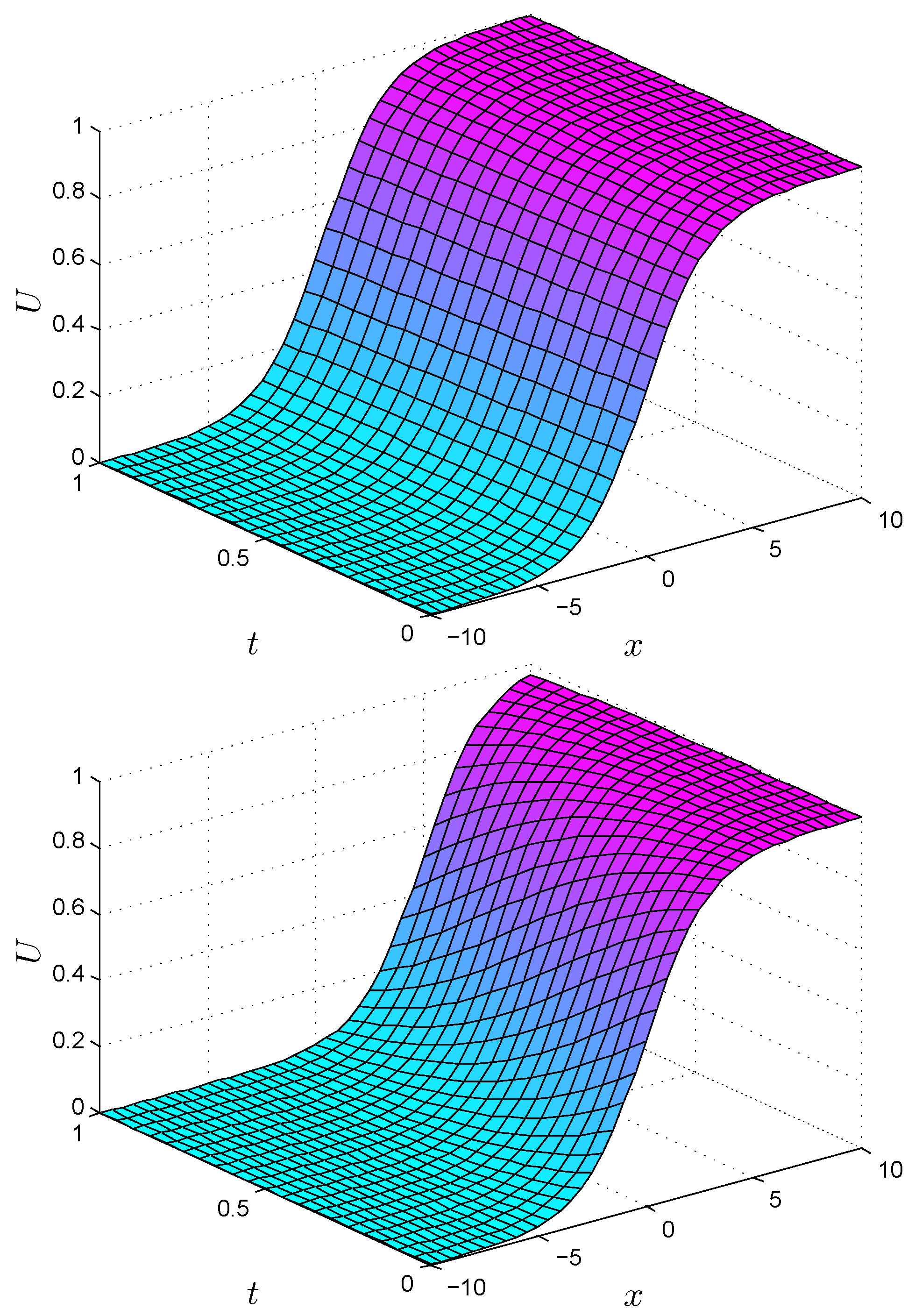
5.0	1.8964 × ${10}^{-4}$	1.8803 × ${10}^{-4}$	2.3050 × ${10}^{-3}$	7.8638 × ${10}^{-4}$

, Figure 1 and Figure 2 and the results are compared with the method reported in [27]. Numerical results of coupled KdV equations are presented in

Table 9. Comparisons between the results obtained by the LMM with those adapted from [29] in term of $L_2$ error norm for Test Problem 7.

t	0.1	0.2	0.3	0.4	0.5	1	2
[29]
U	3.662 × ${10}^{-5}$	5.177 × ${10}^{-5}$	4.065 × ${10}^{-5}$	3.951 × ${10}^{-5}$	3.964 × ${10}^{-5}$	3.975 × ${10}^{-5}$	4.461 × ${10}^{-5}$
V	2.584 × ${10}^{-6}$	3.648 × ${10}^{-6}$	2.855 × ${10}^{-6}$	2.769 × ${10}^{-6}$	2.772 × ${10}^{-6}$	2.749 × ${10}^{-6}$	3.033 × ${10}^{-6}$
EEM
U	8.3147 × ${10}^{-8}$	3.3251 × ${10}^{-7}$	7.4809 × ${10}^{-7}$	1.3299 × ${10}^{-6}$	2.0779 × ${10}^{-6}$	8.3112 × ${10}^{-6}$	3.3245 × ${10}^{-5}$
V	5.8794 × ${10}^{-9}$	2.3512 × ${10}^{-8}$	5.2898 × ${10}^{-8}$	9.4037 × ${10}^{-8}$	1.4693 × ${10}^{-7}$	5.8769 × ${10}^{-7}$	2.3508 × ${10}^{-6}$

and the results are compared with the method given in [29] while numerical results of Hirota-Satsuma coupled KdV equation are shown in

Table 10. Numerical results of the EEM in form of $L_{\infty }$ error norm for Test Problem 8.

k	t	U	V	W
0.1	0.25	4.9097 × ${10}^{-5}$	1.7702 × ${10}^{-8}$	1.7702 × ${10}^{-8}$
	0.50	9.8195 × ${10}^{-5}$	3.6410 × ${10}^{-8}$	3.6410 × ${10}^{-8}$
	0.75	1.4729 × ${10}^{-4}$	5.6117 × ${10}^{-8}$	5.6117 × ${10}^{-8}$
	1.00	1.9639 × ${10}^{-4}$	7.6814 × ${10}^{-8}$	7.6814 × ${10}^{-8}$
	5.00	9.8258 × ${10}^{-4}$	6.0675 × ${10}^{-7}$	6.0675 × ${10}^{-7}$
0.05	0.25	5.2245 × ${10}^{-6}$	2.2740 × ${10}^{-9}$	2.2740 × ${10}^{-9}$
	0.50	1.0464 × ${10}^{-5}$	4.5679 × ${10}^{-9}$	4.5679 × ${10}^{-9}$
	0.75	1.5720 × ${10}^{-5}$	6.8820 × ${10}^{-9}$	6.8820 × ${10}^{-9}$
	1.00	2.0991 × ${10}^{-5}$	9.2162 × ${10}^{-9}$	9.2162 × ${10}^{-9}$
	5.00	1.0741 × ${10}^{-4}$	4.9335 × ${10}^{-8}$	4.9335 × ${10}^{-8}$

. Numerical simulation of reaction-diffusion Brusselator system are shown in

Table 11. Comparisons between the results obtained by the LMM with those adapted from [38,41] using GA RBF at point $(0.40,0.60)$ for Test Problem 9.

		U				V
t	CPU Time	EEM	[38]	[41]	Exact	EEM	[38]	[41]	Exact
0.30	0.17	0.3167	0.3168	0.3166	0.3166	3.1584	3.158	3.157	3.158
0.60	0.19	0.2726	0.2724	0.2725	0.2725	3.6696	3.669	3.667	3.669
0.90	0.23	0.2346	0.2347	0.2345	0.2346	4.2635	4.263	4.260	4.263
1.20	0.26	0.2019	0.2020	0.2018	0.2019	4.9534	4.953	4.950	4.953
1.50	0.30	0.1738	0.1739	0.1737	0.1738	5.7551	5.755	5.751	5.755
1.80	0.34	0.1496	0.1496	0.1495	0.1496	6.6864	6.686	6.681	6.686

and comparison is made with the methods in [38,41]. All the computations were performed on Dell PC Laptop with an Intel(R) Core(TM)i5-2450M CPU 2.50GHz 2.50GHz 4 GB RAM.

Problem 1.

The exact solution [3] of the 1D Lax’s fifth order KdV Equation (1) is

$$U(x,t)=2k^2\left(2-3{tanh}^2\left(k(x-56k^{4}t-x_0)\right)\right),x\in [-10,10],t\ge 0$$

(26)

where the initial and boundary conditions are extracted from the exact solution (26).

Numerical results for Test Problem 1 are given in Table 1 using $k=0.01$, $x_0=0$, $\Delta t=0.01$, $N=11$ and shape parameter $c=100$. Table 1 indicated that the results produced by the LMM using EEM are more better than the method in [3].

Problem 2.

The 1D Lax’s seventh order KdV Equation (2) having exact solution [9]

$$U(x,t)=2k^{2}sec{h}^2\left(k(x-64k^{6}t)\right),x\in [-100,100],t\ge 0$$

(27)

where the initial and boundary equations are extracted from the exact solution (27).

To demonstrate the accuracy and efficiency of the proposed LMM, we reported numerical results in Table 2 for Test Problem 2, in form of $L_{\infty }$ error norm using different values of k and t. We have used EEM with $\Delta t=0.01$, $N=11$ using MQ RBF ($c=100$). From Table 2, one can observe that the LMM is accurate and efficient.

Problem 3.

The 1D generalized Burgers’ Huxley equation (3) having exact solution taken from [52] is given by

$$U(x,t)={\left(\frac{\gamma }{2}+\frac{\gamma }{2}tanh\left({\omega }_1(x-{\omega }_{2}t)\right)\right)}^{\frac{1}{\delta }},a\le x\le b,t\ge 0,$$

(28)

where

$$\begin{array}{c}\hfill {\omega }_1=\frac{-\alpha \delta +\delta \sqrt{{\alpha }^2+4\beta (1+\delta )}}{4(1+\delta )}\gamma ,{\omega }_2=\frac{\alpha \gamma }{1+\delta }-\frac{(1+\delta -\gamma )(-\alpha +\sqrt{{\alpha }^2+4\beta (1+\delta )})}{2(1+\delta )},\end{array}$$

where α, β, δ and γ are constants such that $\beta \ge 0$, $\delta >0$, $\gamma \in (0,1)$.

The initial and boundary conditions are drawn out from the exact solution (28).

In Table 3, we have compared the results obtained by the LMM for generalized Burgers’ Huxley equation for Test Problem 3 with the methods given in [12,14,15]. We have used the parameters values $\alpha =\beta =\delta =1$ and $\gamma =0.001$ and time step length $\Delta t=0.0001$, spatial domain $[-10,20]$, $N=61$ using IMQ RBF. From Table 3, we have noted that the RK4 produced more accurate results than the results reported in [12,14,15].

Table 4 also shows the comparison of numerical results produced by the LMM with the results of Haar wavelet method given in [13]. In the table we have calculated the absolute errors for different values of x and $\delta$ with $\alpha =\beta =1$, $\gamma =0.001$, and $t=0.8$ using IMQ RBF. It can be observed from the table that the LMM is more accurate than the method reported in [13].

The numerical results of Huxley equation for Test Problem 3 with spatial domain $[-10,20]$, $N=61$, $\Delta t=0.01$ and different values of x and t are shown in Table 5. We have used IMQ radial basis function and $\beta =\delta =1$, $\gamma =0.001$. The numerical simulations have carried out by using the RK4 and comparison is done with [14,15] in Table 5. From the table, we have noticed that the results produced by the LMM are better than the methods reported in [14,15].

Problem 4.

The exact solution [18] of the 1D Huxley Equation (4) with $\alpha =\gamma =1$ is given below as

$$U(x,t)=\frac{1}{2}+\frac{1}{2}tanh\left(\frac{1}{2\sqrt{2}}(x-\frac{t}{\sqrt{2}})\right),a\le x\le b,t\ge 0.$$

(29)

The numerical simulations have carried out for Test Problem 4 in Table 6 for different values of t, x, a, b and for $N=10$, $\Delta t=0.0001$ using MQ RBF with $c=5$. The results are obtained by the EEM and compared with the results obtained by Chebyshev spectral collocation method in [19] and found that the results of the LMM are superior.

Problem 5.

The exact solution of the 1D generalized Burgers’ Fisher Equation (5) is given below as

$$U(x,t)={\left(\frac{1}{2}+\frac{1}{2}tanh\left(a_1(x-a_{2}t)\right)\right)}^{\frac{1}{\delta }},a\le x\le b,t\ge 0,$$

(30)

where

$$\begin{array}{c}\hfill a_1=\frac{-\alpha \delta }{2(1+\delta )},a_2=\frac{\alpha }{1+\delta }+\frac{\beta (1+\delta )}{\alpha }.\end{array}$$

(31)

The initial and boundary conditions are taken from the exact solution (30).

Numerical results of the LMM using the RK4 for Test Problem 5 is reported in Table 7. To verify the accuracy of the LMM, we have compared the results with the global meshless collocation method based on RBFs [15] and Adomian decomposition method [14]. The absolute errors for different t, x and $N=41$, $\Delta t=0.001$, $\alpha =\beta =0.001$, $\delta =1$, spatial domain $[-20,20]$ using IMQ RBF are given in Table 7. From the table, one can ensure that the results of the LMM are more accurate than the methods given in [14,15].

Problem 6.

The exact solution [27] of the 1D nonlinear standard Fitzhugh-Nagumo equation (6) is

$$U(x,t)=\frac{1}{2}+\frac{1}{2}tanh\left(\frac{1}{2\sqrt{2}}(x-\frac{2\rho -1}{\sqrt{2}}t)\right),x\in [-10,10]t\ge 0.$$

(32)

The initial and boundary conditions are taken from the exact solution (32).

In Table 8 we have calculated numerical results for Test Problem 6 with $N=101$, $\Delta t=0.0001$ using MQ RBF. Table 8 shows $L_{rms}$ and $L_{\infty }$ error norms of the EEM for $q=0.75$. From the table it can be seen that the obtained results are quite agreed with the results given in [27]. Figure 1 shows the comparison of numerical and analytical solutions for $t=0.2,0.4,0.6,0.8,1$, $q=4$ and $N=41$ for Test Problem 6 while Figure 2 shows the numerical simulations of the EEM for $q=0.75$ and $q=4$.

Problem 7.

The exact solution [29] of 1D coupled KdV equation (7) with $\gamma =3$ and $\alpha =\beta$ is

$$\begin{array}{c}\hfill U(x,t)=\frac{\lambda }{\alpha }sec{h}^2\left(\frac{1}{2}\sqrt{\frac{\lambda }{\alpha }}(x-\lambda t)\right),V(x,t)=\frac{\sqrt{\frac{1}{\alpha }}\lambda sec{h}^2\left(\frac{1}{2}\sqrt{\frac{\lambda }{\alpha }}(x-\lambda t)\right)}{\sqrt{2}}.\end{array}$$

(33)

The initial and boundary conditions are drawn out from the exact solution (33).

In Table 9, we have listed numerical simulations of the EEM versus results obtained from RBFs based collocation method [29] for Test Problem 7. The value of the parameters are $\alpha =\beta =\lambda =0.01$ with the spatial domain $[-5,5]$, $N=101$, $\Delta t=0.001$ and for various time t, using MQ radial basis function with $c=100$. From the listed results given in Table 9, we have observed that the results obtained by the EEM are better than the results given in [29].

Problem 8.

The 1D Hirota-Satsuma coupled KdV system (8) with exact solution [32] given below

$$\begin{array}{cc}\hfill U(x,t)& =4k^2{q}_2{tanh}^2\left(\xi \right)-\frac{8k^2{q}_2}{3}-\frac{C}{3},\hfill \\ \hfill V(x,t)& =2k^2{q}_2{tanh}^2\left(\xi \right)-\frac{2k^2{q}_2}{3}-\frac{4}{3}-c_0,\hfill \\ \hfill W(x,t)& =2k^2{q}_2{tanh}^2\left(\xi \right)-2k^2{q}_2+c_0.\hfill \end{array}$$

(34)

where $\xi =\sqrt{q_2}k(x-Ct)$ and $a\le x\le b$.

The boundary and the initial conditions are obtained from the exact solutions (34).

In Table 10 the numerical simulations of Hirota-Satsuma coupled KdV system (8) are carried out for Test problem 8 on the interval $[-30,30]$ and different values of k and t, with $N=13$, $\Delta t=0.05$, using MQ RBF with $c=2$. The value of parameters $C=c_0=q_2=0.1$. A full agreement between numeric and exact solution have been observed.

Problem 9.

The analytic solution of the 2D reaction-diffusion Brusselator system (9) for a particular case in the region $(x,y)\in {[0,1]}^2$, $t\ge 0$ with $\alpha =1$, $\beta =0$, $\gamma =0.25$ is given in [41]

$$\begin{array}{c}\hfill U(x,y,t)=exp\left(-x-y-\frac{t}{2}\right),V(x,y,t)=exp\left(x+y+\frac{t}{2}\right).\end{array}$$

(35)

The initial and boundary condition are taken from the exact solution (35).

The LMM is employed for the numerical solution of Test Problem 9 by letting time step length $\Delta t=0.001$, the shape parameter value $c=1$, $N=20\times 20$, at various times up to $t=1.8$. In Table 11 we have compared the results obtained by the EEM with the exact solution as well as with [38,41]. Reasonably good accuracy has been obtained in this case as well also CPU time in seconds are reported in the same table.

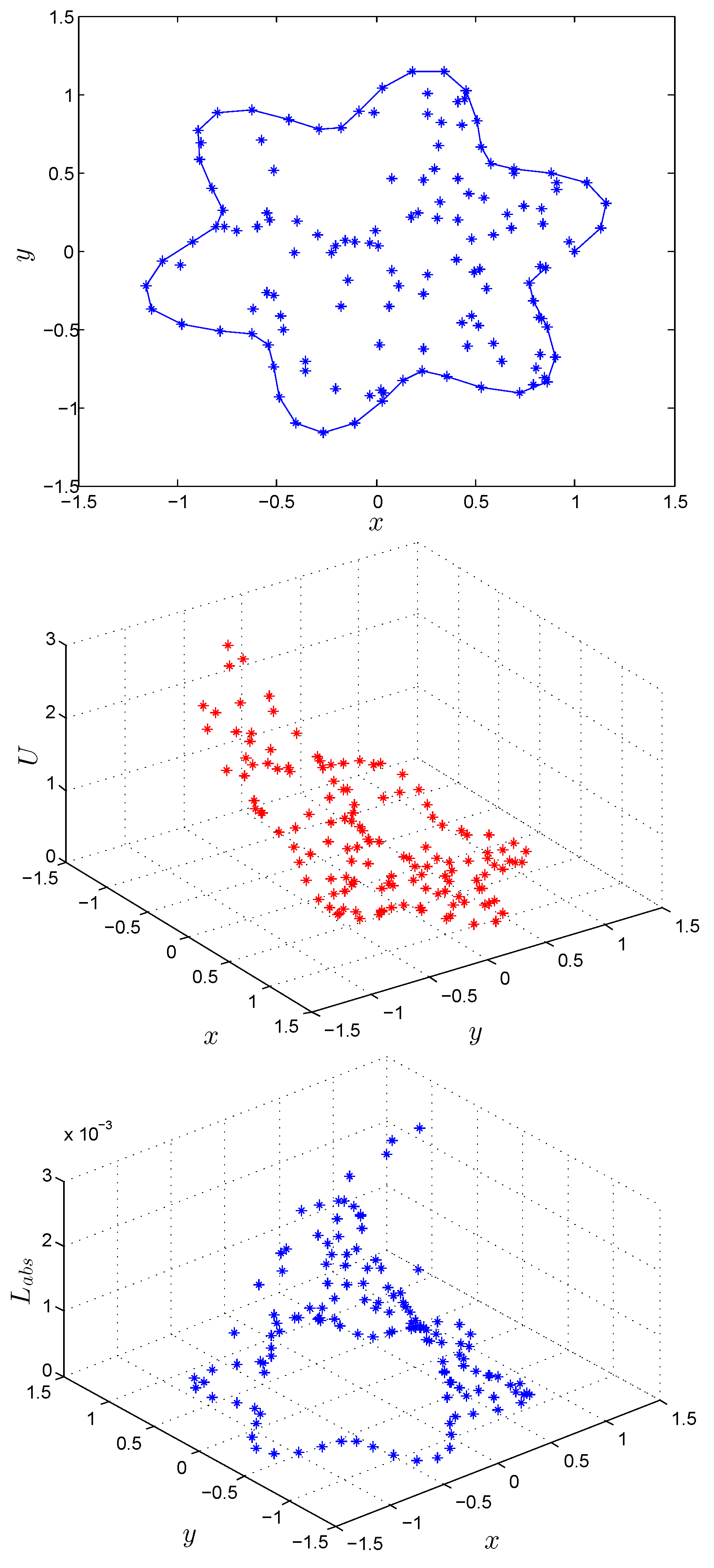
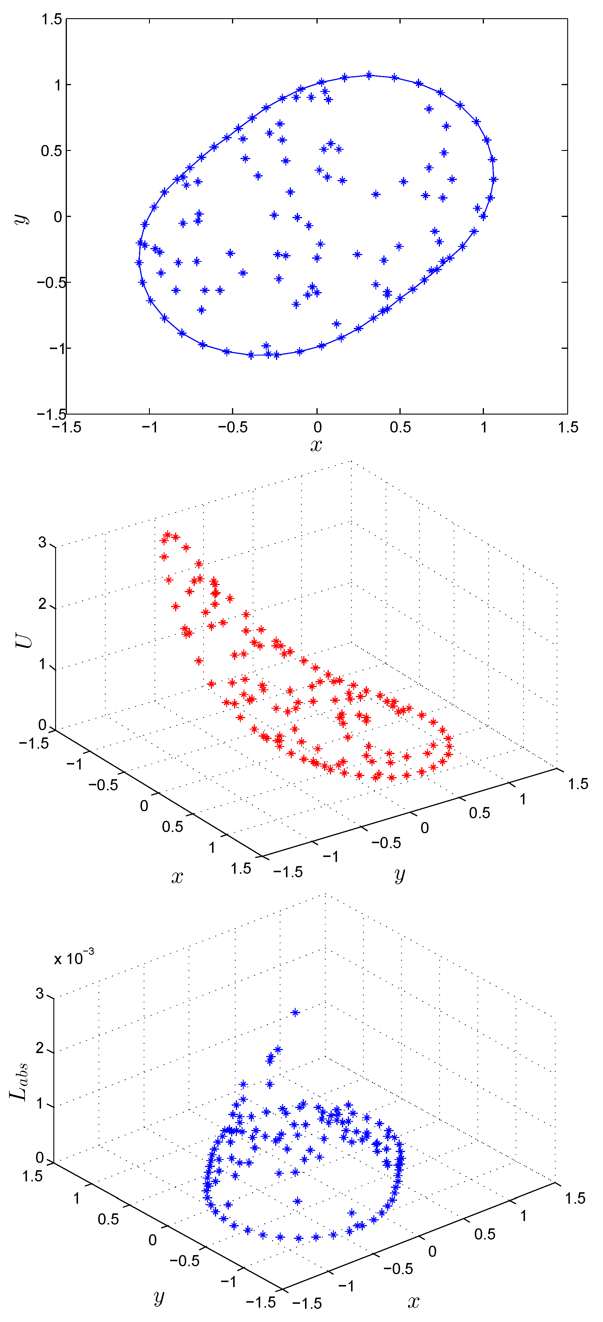
The numerical results on irregular domains are shown in Figure 3, Figure 4, Figure 5 and Figure 6 for Test Problem 9 using MQ RBF with shape parameter $c=1$. The numerical solutions shown in Figure 3, Figure 4, Figure 5 and Figure 6 are performed with $\Delta t=0.001$, $t=1$$\alpha =1$, $\beta =0$ and $\mu =0.25$. These figures show the efficiency of the suggested method in irregular geometry in term of absolute error $L_{abs}$ by using the EEM for Test Problem 9.

5. Conclusions

In this work, a local meshless differential quadrature collocation method is proposed for numerical solution of different mathematical models arising in science and engineering. These models have been solved in the literature by using various numerical methods but our proposed scheme LMM is efficient and accurate on both regular and irregular domains. Results of the LMM are compared with exact or approximate solutions (which ever is available) in the existence literature. On the basis of these results and comparison, we can conclude that the proposed local meshless method is accurate, efficient and its implementation is very simple, straightforward, irrespective of the dimension and geometry of the problem in hand.

References

1. Yamaoto, Y.; Takizawa, E. On a Solution on Non-Linear Time-Evolution Equation of Fifth-Order. J. Phys. Soc. Jpn. 1981, 50, 1421–1422. [Google Scholar] [CrossRef]
2. Djidjeli, K.; Price, W.G.; Twizell, E.H.; Wang, Y. Numerical Methods for the Soltution of the Third and Fifth-Order Disprsive Korteweg-de Vries Equations. J. Comput. Appl. Math. 1995, 58, 307–336. [Google Scholar] [CrossRef]
3. Bakodah, H.O. Modified Adomain Decomposition Method for the Generalized Fifth Order KdV Equations. Am. J. Comput. Math. 2013, 3, 53–58. [Google Scholar] [CrossRef]
4. Kaya, D. An Explicit and Numerical Solutions of Some Fifth-Order KdV Equation by Decomposition Method. Appl. Math. Comput. 2003, 144, 353–363. [Google Scholar] [CrossRef]
5. Goswami, A.; Singh, J.; Kumar, D. Numerical simulation of fifth order KdV equations occurring in magneto- acoustic waves. Ain Shams Eng. J. 2017, 9, 2265–2273. [Google Scholar] [CrossRef]
6. Helal, M.A.; Mehanna, M.S. A Comparative Study between Two Different Methods for Solving the General Korteweg-de Vries Equation (GKDV). Chaos Solitons Fractals 2007, 33, 725–739. [Google Scholar] [CrossRef]
7. Pomeau, Y.; Ramani, A.; Grammaticos, B. Structural stability of the Korteweg-de Vries solitons under a singular perturbation. Phys. D 1988, 31, 127–134. [Google Scholar] [CrossRef]
8. Soliman, A.A. A numerical simulation and explicit solutions of KdVBurgers’ and Lax’s seventh-order KdV equations. Chaos Solitons Fractals 2006, 29, 294–302. [Google Scholar] [CrossRef]
9. Darvishia, M.T.; Kheybari, S.; Khani, F. A Numerical Solution of the Lax’s 7th-order KdV Equation by Pseudospectral Method and Darvishi’s Preconditioning. Int. J. Contemp. Math. Sci. 2007, 2, 1097–1106. [Google Scholar] [CrossRef]
10. El-Sayed, S.M.; Kaya, D. An application of the ADM to seven-order Sawada-Kotara equations. Appl. Math. Comput. 2004, 157, 93–104. [Google Scholar] [CrossRef]
11. Satsuma, J. Topics in Soliton Theory and Exactly Solvable Nonlinear Equations; World Scientific: Singapore, 1987. [Google Scholar]
12. Al-Rozbayani, A.M.; Al-Amr, M.O. Discrete Adomian Decomposition Method for Solving Burgers’-Huxley Equation. Int. J. Contemp. Math. Sci. 2013, 8, 623–631. [Google Scholar] [CrossRef]
13. Celik, I. Haar wavelet method for solving generalized Burgers’-Huxley equation. Arab J. Math. Sci. 2012, 18, 25–37. [Google Scholar]
14. Ismail, H.N.A.; Raslan, K.R.; Rabboh, A.A.A. Adomian decomposition method for Burgers’-Huxley and Burgers’-Fisher equations. Appl. Math. Comput. 2004, 159, 291–301. [Google Scholar]
15. Khattak, A.J. A computational meshless method for the generalized Burgers’-Huxley equation. Appl. Math. Model. 2009, 33, 3718–3729. [Google Scholar] [CrossRef]
16. Bukhari, M.; Arshad, M.; Batool, S.; Saqlain, S.M. Numerical solution of generalized Burger’s-Huxley equation using local radial basis functions. Int. J. Adv. Appl. Sci. 2017, 4, 1–11. [Google Scholar] [CrossRef] [Green Version]
17. Hodgkin, A.L.; Huxley, A.F. A Quantitative Description of Ion Currents and Its Applications to Conduction and Excitation in Nerve Membranes. J. Physiol. 1952, 117, 500–544. [Google Scholar] [CrossRef] [PubMed]
18. Babolian, E.; Saeidian, J. Analytic approximate solutions to Burgers’, Fisher, Huxley equations and two combined forms of these equations. Commun. Nonlinear Sci. Numerical Simul. 2009, 14, 1984–1992. [Google Scholar] [CrossRef]
19. Ashrafi, S.; Alineia, M.; Kheiri, H.; Hojjati, G. Spectral Collocation Method for the Numerical Solution of the Gardner and Huxley Equations. Int. J. Nonlinear Sci. 2014, 18, 71–77. [Google Scholar]
20. Fisher, R.A. The Wave of Advance of Advantageous Genes. Ann. Eugenics 1937, 7, 355–369. [Google Scholar] [CrossRef]
21. Moghimia, M.; Hejazi, F.S.A. Variational iteration method for solving generalized Burgers’-Fisher and Burgers’ equations. Chaos Solitons Fractals 2007, 33, 1756–1761. [Google Scholar] [CrossRef]
22. Javidi, M. Modified pseudospectral method for generalized Burgers’-Fisher equation. Int. Math. Forum 2006, 32, 1555–1564. [Google Scholar] [CrossRef]
23. Mittal, R.C.; Tripathi, A. Numerical solutions of generalized Burgers–Fisher and generalized Burgers–Huxley equations using collocation of cubic B-splines. Int. J. Comput. Math. 2015, 92, 1053–1077. [Google Scholar] [CrossRef]
24. Bhrawy, A.H. A Jacobi-Gauss-Lobatto collocation method for solving generalized Fitzhugh-Nagumo equation with time-dependent coefficients. Appl. Math. Comput. 2013, 222, 255–264. [Google Scholar] [CrossRef]
25. Abbasbandy, S. Soliton solutions for the Fitzhugh-Nagumo equation with the homotopy analysis method. Appl. Math. Model. 2008, 32, 2706–2714. [Google Scholar] [CrossRef]
26. Hariharan, G.; Kannan, K. Haar wavelet method for solving FitzHugh-Nagumo equation. World Acad. Sci. 2010, 43, 560–564. [Google Scholar]
27. Jiwari, R.; Gupta, R.K.; Kumar, V. Polynomial differential quadrature method for numerical solutions of the generalized Fitzhugh-Nagumo equation with time-dependent coefficients. Ain Shams Eng. J. 2014, 5, 1343–1350. [Google Scholar] [CrossRef]
28. Hirota, R.; Satsuma, J. Soliton solutions of a coupled Kortewege-de Vries equation. Phys. Lett. A 1981, 85, 407–418. [Google Scholar] [CrossRef]
29. Haq, S.; Uddin, M. A meshfree interpolation method for the numerical solution of the coupled nonlinear partial differential equations. Eng. Anal. Boundary Elements 2009, 33, 399–409. [Google Scholar]
30. Haq, S.; Hussain, A.; Uddin, M. RBFs Meshless Method of Lines for the Numerical Solution of Time- Dependent Nonlinear Coupled Partial Differential Equations. Appl. Math. 2011, 2, 414–423. [Google Scholar] [CrossRef]
31. Assas, L.M.B. Variational Iteration Method for Solving Coupled-KdV Equations. Chaos Solitons Fractals 2008, 38, 1225–1228. [Google Scholar] [CrossRef]
32. Khater, A.H.; Temsah, R.S.; Callebaut, D.K. Numerical solutions for some coupled nonlinear evolution equations by using spectral collocation method. Math. Comput. Model. 2008, 48, 1237–1253. [Google Scholar] [CrossRef]
33. Wu, Y.T.; Geng, X.G.; Hu, X.B.; Zhu, S.M. Generalized Hirota-Satsuma coupled Korteweg-de Vries equation and Miura transformations. Phys. Lett. A 1999, 64, 255–259. [Google Scholar] [CrossRef]
34. Uddin, M.; Haq, S. Application of a Numerical Method Using Radial Basis Functions to Nonlinear Partial Differential Equations. Selcuk J. Appl. Math. 2011, 12, 77–93. [Google Scholar]
35. Ganji, D.D.; Nourollahi, M.; Rostamian, M. A Comparison of Variational Iteration Method with Adomian’s Decomposition Method in Some Highly Nonlinear Equations. Int. J. Sci. Technol. 2007, 2, 179–188. [Google Scholar]
36. Lefever, R.; Nicolis, G. Chemical instabilities and sustained oscillations. J. Theor. Biol. 1971, 30, 267–284. [Google Scholar] [CrossRef]
37. Tyson, J. Some further studies of nonlinear oscillations in chemical systems. J. Chem. Phys. 1973, 58, 3919. [Google Scholar] [CrossRef]
38. Ali, A.; Haq, S. A computational modeling of the behavior of the two-dimensional reaction-diffusion Brusselator system. Appl. Math. Model. 2010, 34, 3896–3909. [Google Scholar]
39. Wazwaz, A.M. The decomposition method applied to systems of partial differential equations and to the reaction-diffusion Brusselator model. Appl. Math. Comput. 2000, 110, 251–264. [Google Scholar] [CrossRef]
40. Adomian, G. The diffusion Brusselator equation. Comput. Math. Appl. 1995, 29, 1–3. [Google Scholar] [CrossRef]
41. Whye-Teong, A. The two-dimensional reaction-diffusion Brusselator system: a dual-reciprocity boundary element solution. Eng. Anal. Boundary Elements 2003, 27, 897–903. [Google Scholar]
42. Thounthong, P.; Khan, M.N.; Hussain, I.; Ahmad, I.; Kumam, P. Symmetric Radial Basis Function Method for Simulation of Elliptic Partial Differential Equations. Mathematics 2018, 6, 327. [Google Scholar] [CrossRef]
43. Ahmad, I. Local meshless method for PDEs arising from models of wound healing. Appl. Math. Model. 2017, 48, 688–710. [Google Scholar]
44. Ahmad, I.; Riaz, M.; Ayaz, M.; Arif, M.; Islam, S.; Kumam, P. Numerical Simulation of Partial Differential Equations via Local Meshless Method. Symmetry 2019, 11, 257. [Google Scholar] [CrossRef]
45. Aziz, I. Meshless methods for multivariate highly oscillatory Fredholm integral equations. Eng. Anal. Boundary Elements 2015, 53, 100–112. [Google Scholar]
46. Din, Z.-u. Meshless methods for one-dimensional oscillatory Fredholm integral equations. Appl. Math. Comput. 2018, 324, 156–173. [Google Scholar]
47. Din, Z.-u. Meshless methods for two-dimensional oscillatory Fredholm integral equations. J. Comput. Appl. Math. 2018, 335, 33–50. [Google Scholar]
48. Ahmad, I.; Khaliq, A.Q.M. Local RBF method for multi-dimensional partial differential equations. Comput. Math. Appl. 2017, 74, 292–324. [Google Scholar] [CrossRef]
49. FitzHugh, R. Impulses and physiological states in theoretical models of nerve membrane. Biophys. J. 1961, 1, 445–466. [Google Scholar] [CrossRef]
50. Nagumo, J.S.; Arimoto, S.; Yoshizawa, S. An active pulse transmission line simulating nerve axon. Proc. IRE 1962, 50, 2061–2070. [Google Scholar] [CrossRef]
51. Ahmad, I. A comparative analysis of local meshless formulation for multi-asset option models. Eng. Anal. Boundary Elements 2016, 65, 159–176. [Google Scholar]
52. Wang, X.Y.; Zhu, Z.S.; Lu, Y.K. Solitary wave solutions of the generalized Burgers’-Huxley equation. J. Phys. A Math. Theor. 1990, 23, 271–274. [Google Scholar]
Figure 1. Comparing the curves of the numerical and analytical solutions for N = 41 , q = 4 for Test Problem 6.
Mathematics 07 00216 g001
Figure 2. (a) Numerical solutions for q = 0.75 ; (b) Numerical solutions for q = 4 using the EEM for N = 41 , t = 1 for Test Problem 6.
Mathematics 07 00216 g002
Figure 3. Computational domain (a), numerical solution (b) and absolute error (c) by using the EEM for Test Problem 9.
Mathematics 07 00216 g003
Figure 4. Computational domain (a), numerical solution (b) and absolute error (c) by using the EEM for Test Problem 9.
Mathematics 07 00216 g004
Figure 5. Computational domain (a), numerical solution (b) and absolute error (c) by using the EEM for Test Problem 9.
Mathematics 07 00216 g005
Figure 6. Computational domain (a), numerical solution (b) and absolute error (c) by using the EEM for Test Problem 9.
Mathematics 07 00216 g006