Robust H_∞ Control For Uncertain Singular Neutral Time-Delay Systems

Abstract

The present paper attempts to investigate the problem of robust H${}_{\infty }$ control for a class of uncertain singular neutral time-delay systems. First, a linear matrix inequality (LMI) is proposed to give a generalized asymptotically stability condition and an H${}_{\infty }$ norm condition for singular neutral time-delay systems. Second, the LMI is utilized to solve the robust H${}_{\infty }$ problem for singular neutral time-delay systems, and a state feedback control law verifies the solution. Finally, four theorems are formulated in terms of a matrix equation and linear matrix inequalities.

1. Introduction

Singular systems are more convenient than regular ones for describing many practical systems because a singular system involves both differential equations and algebraic equations. Applications of singular systems can be found in circuit systems, chemical systems, biological systems, robot systems, and power systems [1]. Therefore, many scholars have paid attention to the study of singular systems, and a number of important results have been reported (see, e.g., [2,3,4]).

As is known to all, a time delay frequently arises in practical systems and is often the cause of instability and poor performance. Hence, the stability problem for a singular system with a time delay has attracted many researchers’ attention in the past several decades (see, e.g., [5,6,7,8,9,10]).

In some real physical systems and industrial systems, disturbances that are attributable to external signals may cause instability and degrade the system’s performance. Hence, the effect of disturbances on the considered systems should be taken into account. Since H${}_{\infty }$ control is used to keep systems less sensitive to disturbances, problems of H${}_{\infty }$ control for time-delay systems have been widely explored, and findings related to these problems have been reported many times in the literature [11,12,13,14,15,16,17,18,19,20,21,22,23,24,25] as a result of their frequent applications in power systems, large-scale systems, and circuit systems. Recently, scholars (such as [11,12,13,14,15]) have started to study the H${}_{\infty }$ problem for singular time-delay systems by using a linear matrix inequality ($LMI$) approach, which yields not only the existence conditions valid for singular systems’ regular problems but also characterizations of H${}_{\infty }$ controllers, leading to a convex optimization problem [16,17,18,19,20,21,22,23,24,25,26,27,28,29].

The robust H${}_{\infty }$ control problem for uncertain singular time-delay systems was investigated by Ji et al. in [24], where the $LMI$ condition was obtained by constructing a degenerate Lyapunov function on the basis of [23]. However, the condition does not satisfy $\parallel {\tilde{A}}_{d22}\parallel <1$, which renders the design procedure of the LMI law comparatively untenable. Moreover, the problem for singular neutral time-delay systems was not investigated in [24], and some information about the condition itself cannot be revealed even if the method can be applied to a singular neural time-delay system. Also, because of the continuity of the function, it is more difficult to study the neural time-delay system than it is to study singular time-delay systems. Consequently, it is of more theoretical and practical significance to study singular neutral time-delay systems as compared with time-delay systems.

The present paper derives a sufficient condition for the existence of the H${}_{\infty }$ controller on the basis of the $LMI$ approach combined with a class of novel augmented Lyapunov functions, which thus facilitate the attainment of the H${}_{\infty }$ controller using the Matlab $LMI$ toolbox combined with a matrix equation.

2. Problem Statement and Preliminaries

Consider the following uncertain singular neutral time-delay system:

$$\begin{array}{ccc}\hfill E\dot{x}-(C+\Delta C)\dot{x}(t-\tau )& =& (A+\Delta A)x(t)+(A_{\tau }+\Delta A_{\tau })x(t-\tau )\hfill \\ & +& (B+\Delta B)u(t)+B_{\omega }\omega (t),\hfill \\ \hfill z(t)& =& Dx(t),\hfill \\ \hfill x(t)& =& \Phi (t),t\in [-\tau ,0],\hfill \\ \hfill \dot{x}(t)& =& \dot{\Phi }(t),t\in [-\tau ,0],\hfill \end{array}$$

(1)

where $x(t)\in R^n$ is the state vector; $u(t)\in R^m$ is the control input vector; $\omega (t)\in R^p$ is the disturbance input vector belonging to $L_2[0,+\infty )$; $z(t)\in R^q$ is the control output vector; $\tau >0$ is a constant time delay; $\Phi (t)$ is a vector-valued initial function belonging to $C^1([-\tau ,0],R^n);$ $E,C,A,A_{\tau },B,B_{\omega },D$ are constant matrices with appropriate dimensions, where E may be singular and is assumed to be $rankE=r<n$; and $\Delta A,\Delta A_{\tau },\Delta B,B_{\omega }$ are unknown matrices representing time-varying parameter uncertainties and can be described as

$$\begin{array}{c}\hfill [\Delta A,\Delta A_{\tau },\Delta B,\Delta C]=GF(t)[N_a,N_{\tau },N_b,N_c],\end{array}$$

(2)

where G and $N_a,N_{\tau },N_b,N_c$ are known constant matrices and $F:R^{+}\to R^{m\times n}$ is a known matrix with Lebesgue measurable elements and satisfies

$$\sigma (F(t))\le 1.$$

(3)

It is assumed in the present paper that $\parallel \Gamma \dot{x}(t)\parallel \le \parallel \Gamma x(t)\parallel$ for the arbitrary positive-definite matrix $\Gamma$.

The parametric uncertainties $\Delta A,\Delta A_{\tau },\Delta B,\Delta C$ are said to be admissible if Equations (2) and (3) both hold.

Next is a discussion of the system in Equation (1) with no force counterpart item. First, the system is described as Equation (4),

$$\begin{array}{ccc}\hfill E\dot{x}-C\dot{x}(t-\tau )& =& Ax(t)+A_{\tau }x(t-\tau )\hfill \\ \hfill z(t)& =& Dx(t),\hfill \\ \hfill x(t)& =& \Phi (t),t\in [-\tau ,0],\hfill \\ \hfill \dot{x}(t)& =& \dot{\Phi }(t),t\in [-\tau ,0].\hfill \end{array}$$

(4)

The following definitions and lemmas are very useful for deriving the main results of this paper.

Definition 1

([1]). $(1):$ The pair (E, A) is known as regular if $det(sE-A)$ is not identically zero. $(2):$ The pair $(E,A)$ is known as impulse free if $det(sE-A)=rank(E)$.

Definition 2

([24]). The singular neutral time-delay system (Equation (4)) is known as regular and impulse free if the pair $(E,A)$ is regular and impulse free.

Remark 1.

The regularity and impulses of the pair $(E,A)$ ensure the system (Equation (4)) with $\tau \ne 0$ to be regular and impulse free, and they further ensure the existence of a unique solution to the system in Equation (4) on $[-\tau ,+\infty ).$

Since $(E,A)$ is regular and impulse free, there exist two nonsingular matrices Q and P such that the system in Equation (4) is equivalent to

$$\begin{array}{ccc}\hfill {\dot{x}}_1(t)& =& A_1{x}_1(t)+A_{\tau 11}{x}_1(t-\tau )+A_{\tau 12}{x}_2(t-\tau )+C_{11}{\dot{x}}_1(t-\tau )+C_{12}{\dot{x}}_2(t-\tau ),\hfill \\ \hfill 0& =& x_2(t)+A_{\tau 21}{x}_1(t-\tau )+A_{\tau 22}{x}_2(t-\tau )+C_{21}{\dot{x}}_1(t-\tau )+C_{22}{\dot{x}}_2(t-\tau ),\hfill \end{array}$$

(5)

with the coordinate transformation

$$\left[\begin{array}{c}{x}_1\hfill \\ x_2\hfill \end{array}\right]=P^{-1}x,x_1\in R^{n_1},x_2\in R^{n_2}$$

and

$$QEP=diag(I_{n_1},0),QAP=diag(A_1,I_{n_2})$$

$$Q{A}_{\tau }P=\left[\begin{array}{cc}{A}_{{\tau }_{11}}& A_{{\tau }_{12}}\\ A_{{\tau }_{21}}& A_{{\tau }_{22}}\end{array}\right],QCP=\left[\begin{array}{cc}{C}_{11}& C_{12}\\ C_{21}& C_{22}\end{array}\right],$$

where $n_1+n_2=n.$ Obviously, the system in Equation (5) has a unique solution on $[-\tau ,+\infty )$.

Definition 3

([29]). If a matrix X satisfies the Penrose condition $AXA=A$, then there exists a solution to the generalized inverse for $AXA=A$ or $\{1\}$ inverse of A, and thus, the matrix X is denoted by X = A${}^{(1)}$ or X $\in A\{1\}$, where $A\{1\}$ denotes the set of all $\{1\}$ inverse of A.

Lemma 1

([24]). For a given symmetry matrix $A=\left[\begin{array}{cc}{A}_{11}& A_{12}\\ A_{21}& A_{22}\end{array}\right]$, where $A_{11},A_{12},A_{21},A_{22}$ have appropriate dimensions, $A_{21}=A_{12}^T$. Then, the following two conditions are equivalent.

$$C1:A<0C2:A_{22}<0,A_{11}-A_{12}{A}_{22}^{-1}{A}_{21}<0.$$

Lemma 2

([18]). For any $x,y\in R^n,\epsilon >0$, the inequality $2x^{T}y\le \epsilon x^{T}x+\frac{1}{\epsilon }{y}^{T}y$ holds.

Therefore, Lemma 3 can be obtained by using a method similar to that in J. Lee (1994).

Lemma 3.

For given matrices $Q=Q^T,H,E$, and F of appropriate dimensions,

$$Q+HFE+E^T{F}^T{H}^T+{\Psi }_{1}F{\Psi }_2+{\Psi }_2^T{F}^T{\Psi }_1^T+{\Phi }_{1}F{\Phi }_2+{\Phi }_2^T{F}^T{\Phi }_1^T<0,$$

for all F satisfies $F^{T}F\le I$ if there exist positive numbers ${\epsilon }_1>0,{\epsilon }_2>0,{\epsilon }_3>0$ such that

$$Q+{\epsilon }_{1}H{H}^T+{\epsilon }_1^{-1}{E}^{T}E+{\epsilon }_2{\Psi }_1{\Psi }_1^T+{\epsilon }_2^{-1}{\Psi }_2^T{\Psi }_2+{\epsilon }_3{\Phi }_1{\Phi }_1^T+{\epsilon }_3^{-1}{\Phi }_2^T{\Phi }_2<0.$$

Proof. 

By Lemma 2, for $\forall z\in R^n\backslash \{0\},$ there exists an ${\epsilon }_1>0$ such that

$$z^{T}HFEz=\frac{1}{2}\times 2z^{T}HFEz\le \frac{1}{2}{\epsilon }_1{z}^{T}HF{F}^T{H}^{T}z+\frac{1}{2}{\epsilon }_1^{-1}{z}^T{E}^{T}Ez\le \frac{1}{2}{\epsilon }_1{z}^{T}H{H}^{T}z+\frac{1}{2}{\epsilon }_1^{-1}{z}^T{E}^{T}Ez,$$

$$z^T{E}^T{F}^T{H}^{T}z=\frac{1}{2}\times 2z^T{E}^T{F}^T{H}^{T}z\le \frac{1}{2}{\epsilon }_1^{-1}{z}^T{E}^T{F}^{T}FEz+\frac{1}{2}{\epsilon }_1{z}^{T}H{H}^{T}z\le \frac{1}{2}{\epsilon }_1^{-1}{z}^T{E}^{T}Ez+\frac{1}{2}{\epsilon }_1{z}^{T}H{H}^{T}z,$$

hold simultaneously. Thus,

$$HFE+E^T{F}^T{H}^T\le {\epsilon }_{1}H{H}^T+{\epsilon }_1^{-1}{E}^{T}E,$$

can be obtained. Similarly, there exist positive numbers ${\epsilon }_2,{\epsilon }_3$ such that the following inequalities also hold

$${\Psi }_{1}F{\Psi }_2+{\Psi }_2^T{F}^T{\Psi }_1^T\le {\epsilon }_2{\Psi }_1{\Psi }_1^T+{\epsilon }_2^{-1}{\Psi }_2^T{\Psi }_2,$$

$${\Phi }_{1}F{\Phi }_2+{\Phi }_2^T{F}^T{\Phi }_1^T\le {\epsilon }_3{\Phi }_1{\Phi }_1^T+{\epsilon }_3^{-1}{\Phi }_2^T{\Phi }_2.$$

□

Lemma 4

([29]). Let A∈ C${}^{m\times n}$, B∈ C${}^{p\times q}$, D∈ C ${}^{m\times q}$. Then, the matrix equation $AXB=D$ is consistent if and only if, for some A${}^{(1)}$ and B${}^{(1)}$, $A{A}^{(1)}D{B}^{(1)}B=D$ is satisfied, in which case the general solution is $X=A^{(1)}D{B}^{(1)}+Y-A^{(1)}AYB{B}^{(1)}$ for arbitrary Y ∈ C ${}^{n\times p}$.

Robust$H_{\infty }$control problem. The present paper attempts to address the robust $H_{\infty }$ control problem by considering the linear state feedback control law as

$$u(t)=Kx(t)$$

to construct K such that $u(t)$ in Equation $(6)$ will

$(a)$ stabilize the resultant closed-loop system and

$(b)$ guarantee the $H_{\infty }$ performance $J={\int }_0^{\infty }(z^T(t)z(t)-{\gamma }^2{\omega }^T(t)\omega (t))dt<0$ under the zero-initial condition of $x(t)$ and $\dot{x}(t)$ for any nonzero $\omega (t)\in L_2[0,\infty )$ and for all admissible parameter uncertainties satisfying Equations $(2)$ and $(3)$.

3. Results

In the following, the problem of robust $H_{\infty }$ control is considered for the singular neutral system in Equation $(1)$ with $F(t)=0$ and $u(t)=0$.

Theorem 1.

Consider the system in Equation $(1)$ with $F(t)=0$ and $u(t)=0$. For a given scalar $\gamma >0$, the system in Equation $(1)$ is regular, impulse free, and stable, and the $H_{\infty }$ norm from $\omega (t)$ to $z(t)$ is less than γ, if there exist symmetric positive-definite matrices $P,Q,R,L$ and matrices $S,S_{\tau },S_{\omega }$ such that the following linear matrix inequality holds:

$$\begin{array}{c}\hfill \Sigma =\left[\begin{array}{ccccccc}{\Sigma }_{11}& {\Sigma }_{12}& {\Sigma }_{13}& {\Sigma }_{14}& L^T& D^T& A^{T}R\\ \ast & {\Sigma }_{22}& {\Sigma }_{23}& {\Sigma }_{24}& 0& 0& A_{\tau }^{T}R\\ \ast & \ast & {\Sigma }_{33}& {\Sigma }_{34}& 0& 0& C^{T}R\\ \ast & \ast & \ast & {\Sigma }_{44}& 0& 0& B_{\omega }^{T}R\\ \ast & \ast & \ast & \ast & -I& 0& 0\\ \ast & \ast & \ast & \ast & \ast & -I& 0\\ \ast & \ast & \ast & \ast & \ast & \ast & -R\end{array}\right]<0,\end{array}$$

(6)

where

• ${\Sigma }_{11}=E^{T}PA+A^{T}PE+A^{T}V{S}^T+S{V}^{T}A+Q,$
• ${\Sigma }_{12}=E^{T}P{A}_{\tau }+S{V}^T{A}_{\tau }+A^{T}V{S}_{\tau }^T,{\Sigma }_{13}=E^{T}PC+S{V}^{T}C,$
• ${\Sigma }_{14}=E^{T}P{B}_{\omega }+S{V}^T{B}_{\omega }+A^{T}V{S}_{\omega }^T,{\Sigma }_{22}=-Q+S_{\tau }{V}^T{A}_{\tau }+A_{\tau }^{T}V{S}_{\tau }^T,$
• ${\Sigma }_{23}=S_{\tau }{V}^{T}C,{\Sigma }_{24}=S_{\tau },V^T{B}_{\omega }+A_{\tau }^{T}V{S}_{\omega }^T,{\Sigma }_{33}=-E^{T}RE-L^{T}L,$
• ${\Sigma }_{34}=C^{T}V{S}_{\omega }^T,{\Sigma }_{44}=-{\gamma }^{2}I+S_{\omega }{V}^T{B}_{\omega }+B_{\omega }^{T}V{S}_{\omega }^T,$

and $V\in R^{n\times (n-r)}$ is any matrix that has full column rank and satisfies $E^{T}V=0$.

Proof. 

The nonlinear singular system (Equation $(1)$) is proved below to be regular and impulse free. Since rank(E) = r $\le n$, there exist two nonsingular matrices F and G $\in R^{n\times n}$ such that

$$\overline{E}=GEF=\left[\begin{array}{cc}{I}_r& 0\\ 0& 0\end{array}\right]$$

Then, V can be parameterized as

$V=G^T\left[\begin{array}{c}0\\ \overline{\Phi }\end{array}\right],$ where $\overline{\Phi }\in R^{(n-r)\times (n-r)}$ is any nonsingular matrix. Next, $\overline{A}=GAF=\left[\begin{array}{cc}{\overline{A}}_{11}& {\overline{A}}_{12}\\ {\overline{A}}_{21}& {\overline{A}}_{22}\end{array}\right],\overline{P}=G^{-T}P{G}^{-1}=\left[\begin{array}{cc}{\overline{P}}_{11}& {\overline{P}}_{12}\\ {\overline{P}}_{21}& {\overline{P}}_{22}\end{array}\right],\overline{S}=F^{T}S=\left[\begin{array}{c}{\overline{S}}_{11}\\ {\overline{S}}_{21}\end{array}\right],\overline{V}=G^{-T}V=\left[\begin{array}{c}0\\ \overline{\Phi }\end{array}\right]$ can be defined. Since ${\Sigma }_{11}<0$ and $Q>0$, the following inequality can be formulated easily:

$$\Omega =E^{T}PA+A^{T}PE+A^{T}V{S}^T+S{V}^{T}A<0$$

.

Pre- and post-multiplying $\Omega <0$ by F${}^T$ and F, respectively, yields

$$\begin{array}{ccc}\hfill F^T\Omega F& =& {\overline{E}}^T\overline{PA}+{\overline{A}}^T\overline{PE}+{\overline{A}}^T{\overline{VS}}^T+{\overline{SV}}^T\overline{A}\hfill \\ & =& \left[\begin{array}{cc}{\overline{\Omega }}_{11}& {\overline{\Omega }}_{12}\\ {\overline{\Omega }}_{21}& {\overline{A}}_{22}^T\overline{\Phi }{\overline{S}}_{21}^T+{\overline{S}}_{21}{\overline{\Phi }}^T{\overline{A}}_{22}\end{array}\right]<0\hfill \end{array}$$

(7)

From [17], the following matrix inequalities can be formulated easily:

$$\begin{array}{c}\hfill {\overline{A}}_{22}^T\overline{\Phi }{\overline{S}}_{21}^T+{\overline{S}}_{21}{\overline{\Phi }}^T{\overline{A}}_{22}<0,\end{array}$$

(8)

and thus, ${\overline{A}}_{22}$ is nonsingular.

Then, it can be proved that

$$\begin{array}{ccc}\hfill det(sE-A)& =& det(G^{-1})det(s\overline{E}-\overline{A})det(F^{-1})\hfill \\ & =& det(G^{-1})det(-{\overline{A}}_{22})det(s{I}_r-({\overline{A}}_{11}-{\overline{A}}_{12}{\overline{A}}_{22}^{-1}{\overline{A}}_{21}))det(F^{-1}),\hfill \end{array}$$

which implies that $det(sE-A)$ is not identically zero and $deg(det(sE-A))=r=rank(E)$. Then, the pair $(E,A)$ is regular and impulse free, which implies that the system in Equation (1) is regular and impulse free.

In the following, the system in Equation $(1)$ with $u(t)=0$ and $F(t)=0$ is proved to be asymptotical with the condition of $\omega (t)=0$ and an $H_{\infty }$ performance under the zero-initial condition of $x(t)$ and $\dot{x}(t)$ for any nonzero $\omega (t)\in L_2[0,\infty )$. Construct a Lyapunov–Krasovskii function candidate as follows:

$$\begin{array}{c}\hfill V_0(x_t)=x^T(t)E^{T}PEx(t)+{\int }_{t-\tau }^t{x}^T(s)Qx(s)ds+{\int }_{t-\tau }^t{\dot{x}}^T(s)(E^{T}RE+L^{T}L)\dot{x}(s)ds,\end{array}$$

(9)

where P $>0$, Q $>0$, R $>0$, and L $>0$. From this follows the derivation of $V_0(t,x_t)$ with respect to t along the trajectory of the system in Equation $(1)$ with the condition of $F(t)=0$ and $u(t)=0$ that

$$\begin{array}{ccc}\hfill {\dot{V}}_0(x_t)& =& 2{(Ex(t))}^{T}P(E\dot{x}(t))+x^T(t)Qx(t)-x^T(t-\tau )Qx(t-\tau )+{(E\dot{x}(t))}^{T}R(E\dot{x}(t))\hfill \\ & & -{\dot{x}}^T(t-\tau )E^{T}RE\dot{x}(t-\tau )+{\dot{x}}^T(t)L^{T}L\dot{x}(t)-{\dot{x}}^T(t-\tau )L^{T}L\dot{x}(t-\tau )\hfill \\ & =& 2x^T(t)E^{T}P(Ax(t)+A_{\tau }x(t-\tau )+B_{\omega }\omega (t)+C\dot{x}(t-\tau ))+x^T(t)Qx(t)\hfill \\ & & -x^T(t-\tau )Qx(t-\tau )+{(E\dot{x}(t))}^{T}R(E\dot{x}(t))-{\dot{x}}^T(t-\tau )E^{T}RE\dot{x}(t-\tau )\hfill \\ & & +{\dot{x}}^T(t)L^{T}L\dot{x}(t)-{\dot{x}}^T(t-\tau )L^{T}L\dot{x}(t-\tau )\hfill \\ & =& x^T(t)(E^{T}PA+A^{T}PE+Q)x(t)+2x^T(t)E^{T}P{A}_{\tau }x(t-\tau )\hfill \\ & & +2x^T(t)E^{T}P{B}_{\omega }\omega (t)+2x^T(t)E^{T}PC\dot{x}(t-\tau )-x^T(t-\tau )Qx(t-\tau )\hfill \\ & & +{(E\dot{x}(t))}^{T}R(E\dot{x}(t))-{\dot{x}}^T(t-\tau )(E^{T}RE+L^{T}L)\dot{x}(t-\tau )+{\dot{x}}^T(t)L^{T}L\dot{x}(t)\hfill \\ & =& x^T(t)(E^{T}PA+A^{T}PE+Q)x(t)+2x^T(t)E^{T}P{A}_{\tau }x(t-\tau )\hfill \\ & & +2x^T(t)E^{T}P{B}_{\omega }\omega (t)+2x^T(t)E^{T}PC\dot{x}(t-\tau )-x^T(t-\tau )Qx(t-\tau )\hfill \\ & & +{(E\dot{x}(t))}^{T}R(E\dot{x}(t))-{\dot{x}}^T(t-\tau )(E^{T}RE+L^{T}L)\dot{x}(t-\tau )+x^T(t)L^{T}Lx(t).\hfill \end{array}$$

(10)

For the system in Equation $(1)$, the following holds

$$\begin{array}{cc}\hfill {(E\dot{x}(t))}^{T}R(E\dot{x}(t))& ={(Ax(t)+A_{\tau }x(t-\tau )+B_{\omega }\omega (t)+C\dot{x}(t-\tau ))}^{T}R(Ax(t)\hfill \\ \hfill & +A_{\tau }x(t-\tau )+B_{\omega }\omega (t)+C\dot{x}(t-\tau ))\hfill \\ \hfill \end{array}$$

$$\begin{array}{c}=\left[x^T(t)x^T(t-\tau ){\dot{x}}^T(t-\tau ){\omega }^T(t)\right]U\left[\begin{array}{c}x(t)\\ x(t-\tau )\\ \dot{x}(t-\tau )\\ \omega (t)\end{array}\right]\hfill \end{array}$$

(11)

where

$$U=\left[\begin{array}{cccc}{A}^{T}RA& A^{T}R{A}_{\tau }& A^{T}RC& A^{T}R{B}_{\omega }\\ \ast & A_{\tau }^{T}R{A}_{\tau }& A_{\tau }^{T}RC& A_{\tau }^T{B}_{\omega }\\ \ast & \ast & C^{T}RC& C^{T}R{B}_{\omega }\\ \ast & \ast & \ast & B_{\omega }^{T}R{B}_{\omega }\end{array}\right].$$

For ${\mathit{E}}^{\mathit{T}}\mathit{V}=\mathit{0}$, it can be deduced that

$$\begin{array}{cc}\hfill 0& =2(x^T(t)S+x^T(t-\tau )S_{\tau }+{\omega }^T(t)S_{\omega })V^{T}E\dot{x}(t)\hfill \\ \hfill & =2x^T(t)S{V}^T(Ax(t)+A_{\tau }x(t-\tau )+B_{\omega }\omega (t)+C\dot{x}(t-\tau ))\hfill \\ & +2x^T(t-\tau )S_{\tau }{V}^T(Ax(t)+A_{\tau }x(t-\tau )+B_{\omega }\omega (t)+C\dot{x}(t-\tau ))\hfill \\ \hfill & +2{\omega }^T(t)S_{\omega }{V}^T(Ax(t)+A_{\tau }x(t-\tau )+B_{\omega }\omega (t)+C\dot{x}(t-\tau )),\hfill \end{array}$$

(12)

where S is any matrix with appropriate dimensions.

Noting the zero-initial condition of $x(t)$, $V(x_0)=0$, and $V(x_{\infty })>0$, then

$$\begin{array}{cc}\hfill J& ={\int }_0^{\infty }(z^T(t)z(t)-{\gamma }^2{\omega }^T(t)\omega (t))dt\hfill \\ \hfill & \le {\int }_0^{\infty }(z^T(t)z(t)-{\gamma }^2{\omega }^T(t)\omega (t))+{\dot{V}}_0(t,x_t)dt\hfill \\ & ={\int }_0^{\infty }x{(t)}^T{D}^{T}Dx(t)-{\gamma }^2{\omega }^T(t)\omega (t)+{\dot{V}}_0(t,x_t)dt.\hfill \end{array}$$

(13)

By substituting Equations $(10),(11),$ and $(12)$ into $(13)$, the following can be obtained:

$$J\le \left[\begin{array}{c}{x}^T(t)x^T(t-\tau ){\dot{x}}^T(t-\tau ){\omega }^T(t)\end{array}\right]\Theta \left[\begin{array}{c}x(t)\\ x(t-\tau )\\ \dot{x}(t-\tau )\\ \omega (t)\end{array}\right],$$

where $\Theta =\left[\begin{array}{cccc}{\Theta }_{11}& {\Theta }_{12}& {\Theta }_{13}& {\Theta }_{14}\\ \ast & {\Theta }_{22}& {\Theta }_{23}& {\Theta }_{24}\\ \ast & \ast & {\Theta }_{33}& {\Theta }_{34}\\ \ast & \ast & \ast & {\Theta }_{44}\end{array}\right]$, with

• ${\Theta }_{11}=E^{T}PA+A^{T}PE+A^{T}V{S}^T+S{V}^{T}A+Q+L^{T}L+D^{T}D+A^{T}RA,$
• ${\Theta }_{12}=E^{T}P{A}_{\tau }+S{V}^T{A}_{\tau }+A^{T}V{S}_{\tau }^T+A^{T}R{A}_{\tau },$
• ${\Theta }_{13}=E^{T}PC+S{V}^{T}C+A^{T}RC,$
• ${\Theta }_{14}=E^{T}P{B}_{\omega }+S{V}^T{B}_{\omega }+A^{T}V{S}_{\omega }^T+A^{T}R{B}_{\omega },$
• ${\Theta }_{22}=-Q+S_{\tau }{V}^T{A}_{\tau }+A_{\tau }^{T}V{S}_{\tau }^T+A_{\tau }^{T}R{A}_{\tau },$
• ${\Theta }_{23}=S_{\tau }{V}^{T}C+A_{\tau }^{T}RC,$
• ${\Theta }_{24}=S_{\tau }{V}^T{B}_{\omega }+A_{\tau }^{T}V{S}_{\omega }^T+A_{\tau }^{T}R{B}_{\omega },$
• ${\Theta }_{33}=-E^{T}RE-L^{T}L+C^{T}RC,$
• ${\Theta }_{34}=C^{T}V{S}_{\omega }^T+C^{T}R{B}_{\omega },$
• ${\Theta }_{44}=-{\gamma }^{2}I+S_{\omega },$
• $V^T{B}_{\omega }+B_{\omega }^{T}V{S}_{\omega }^T+B_{\omega }^{T}R{B}_{\omega }$.

If $\Theta <0$, there exists a scalar $\lambda >0$ such that $J\le -\lambda \parallel x(t){\parallel }^2$; thus, according to [3], the system in Equation $(1)$ with $u(t)=0$ and $F(t)=0$ is asymptotically stable. By Lemma 1, $\Theta <0$ is equivalent to $\Sigma <0$.

It is easy to obtain from the result of Theorem 1 the following conclusion about the $H_{\infty }$ performance analysis. □

Theorem 2.

Consider the system in Equation $(1)$ with $u(t)=0$. For a given scalar $\gamma >0$, the system is regular, impulse free, and stable, and the $H_{\infty }$ norm from $\omega (t)$ to $z(t)$ is less than γ if there exist symmetric positive-definite matrices P, Q, R, L and matrices $S,S_{\tau },S_{\omega }$, and $\epsilon >0$ such that the following linear matrix inequality holds:

$$\begin{array}{c}\hfill \overline{\Sigma }=\left[\begin{array}{ccccccccc}{\Sigma }_{11}& {\Sigma }_{12}& {\Sigma }_{13}& {\Sigma }_{14}& L^T& D^T& A^{T}R& (E^{T}P+S{V}^T)G& \epsilon N_a^T\\ \ast & {\Sigma }_{22}& {\Sigma }_{23}& {\Sigma }_{24}& 0& 0& A_{\tau }^{T}R& S_{\tau }{V}^{T}G& \epsilon N_{\tau }^T\\ \ast & \ast & {\Sigma }_{33}& {\Sigma }_{34}& 0& 0& C^{T}R& 0& \epsilon N_c^T\\ \ast & \ast & \ast & {\Sigma }_{44}& 0& 0& B_{\omega }^{T}R& S_{\omega }{V}^{T}G& 0\\ \ast & \ast & \ast & \ast & -I& 0& 0& 0& 0\\ \ast & \ast & \ast & \ast & \ast & -I& 0& 0& 0\\ \ast & \ast & \ast & \ast & \ast & \ast & -R& R^{T}G& 0\\ \ast & \ast & \ast & \ast & \ast & \ast & \ast & -\epsilon I& 0\\ \ast & \ast & \ast & \ast & \ast & \ast & \ast & \ast & -\epsilon I\end{array}\right]<0,\end{array}$$

(14)

where ${\Sigma }_{ij}$ is as defined in Theorem 1.

Proof. 

It follows from Equation $(14)$ by Lemma 1 that

$$\begin{array}{c}\hfill \Sigma +{\epsilon }^{-1}\Psi {\Psi }^T+\epsilon {\Phi }^T\Phi <0\end{array}$$

(15)

where $\Sigma$ is as defined in Theorem 1, and

$$\Psi ={[G^{T}PE+G^{T}V{S}^T,G^{T}V{S}_{\tau }^T,0,G^{T}V{S}_{\omega }^T,0,0,G^{T}R]}^T,\Phi =[N_a,N_{\tau },N_c,0,0,0,0]$$

.

It follows from Equation $(15)$ by Lemma 3 that

$$\begin{array}{c}\hfill \left[\begin{array}{ccccccc}{\Omega }_{11}& {\Omega }_{12}& {\Omega }_{13}& {\Omega }_{14}& L^T& D^T& {\Omega }_{17}\\ \ast & {\Omega }_{22}& {\Omega }_{23}& {\Omega }_{24}& 0& 0& {\Omega }_{27}\\ \ast & \ast & {\Omega }_{33}& {\Omega }_{34}& 0& 0& {\Omega }_{37}\\ \ast & \ast & \ast & {\Omega }_{44}& 0& 0& {\Omega }_{47}\\ \ast & \ast & \ast & \ast & -I& 0& 0\\ \ast & \ast & \ast & \ast & \ast & -I& 0\\ \ast & \ast & \ast & \ast & \ast & \ast & -R\end{array}\right]<0,\end{array}$$

(16)

where

• ${\Omega }_{11}=E^{T}P(A+\Delta A)+{(A+\Delta A)}^{T}PE+{(A+\Delta A)}^{T}V{S}^T+S{V}^T(A+\Delta A)+Q,$
• ${\Omega }_{12}=E^{T}P(A_{\tau }+\Delta A_{\tau })+S{V}^T(A_{\tau }+\Delta A_{\tau })+{(A+\Delta A)}^{T}V{S}_{\tau }^T,$
• ${\Omega }_{13}=E^{T}P(C+\Delta C)+S{V}^T(C+\Delta C),$
• ${\Omega }_{14}=E^{T}P{B}_{\omega }+S{V}^T{B}_{\omega }+{(A+\Delta A)}^{T}V{S}_{\omega }^T,$
• ${\Omega }_{17}={(A+\Delta A)}^{T}R,$
• ${\Omega }_{22}=-Q+S_{\tau }{V}^T(A_{\tau }+\Delta A_{\tau })+{(A_{\tau }+\Delta A_{\tau })}^{T}V{S}_{\tau }^T,$
• ${\Omega }_{23}=S_{\tau }{V}^T(C+\Delta C),$
• ${\Omega }_{24}=S_{\tau }{V}^T{B}_{\omega }+{(A_{\tau }+\Delta A_{\tau })}^{T}V{S}_{\omega }^T,$
• ${\Omega }_{27}={(A_{\tau }+\Delta A_{\tau })}^{T}R,$
• ${\Omega }_{33}=-E^{T}RE-L^{T}L,$
• ${\Omega }_{34}={(C+\Delta C)}^{T}V{S}_{\omega }^T,$
• ${\Omega }_{37}={(C+\Delta C)}^{T}R,$
• ${\Omega }_{44}=-{\gamma }^{2}I+S_{\omega }{V}^T{B}_{\omega }+B_{\omega }^{T}V{S}_{\omega }^T,$
• ${\Omega }_{47}=B_{\omega }^{T}R,$

and $V\in R^{n\times (n-r)}$ is any matrix that has full column rank and satisfies $E^{T}V=0$.

In the following, the robust $H_{\infty }$ synthesis problem of the system in Equation $(1)$ is to be considered for the system in Equation $(1)$ with $F(t)=0$. □

Theorem 3.

Consider the system in Equation (1) with $F(t)=0$. For a given scalar $\gamma >0$, if there exist symmetric positive-definite the matrices $P,Q,R,L$ and matrices $S,Y_1,Y_2$ such that the matrix equation and the linear matrix inequality in the following hold simultaneously,

$$\begin{array}{c}\hfill [Y_1,Y_2]{[P{E}^T+V{S}^T,R]}^{(1)}[P{E}^T+V{S}^T,R]=[Y_1,Y_2]\end{array}$$

(17)

$$\begin{array}{c}\hfill \Xi =\left[\begin{array}{ccccccc}{\Xi }_{11}& {\Xi }_{12}& {\Xi }_{13}& {\Xi }_{14}& L^T& B_{\omega }& AR+B{Y}_2\\ \ast & -Q& 0& 0& 0& 0& A_{\tau }R\\ \ast & \ast & -E^{T}RE-L^{T}L& 0& 0& 0& CR\\ \ast & \ast & \ast & -{\gamma }^{2}I& 0& 0& DR\\ \ast & \ast & \ast & \ast & -I& 0& 0\\ \ast & \ast & \ast & \ast & \ast & -I& 0\\ \ast & \ast & \ast & \ast & \ast & \ast & -R\end{array}\right]<0,\end{array}$$

(18)

then, the control law

$$u(t)=(Y_1,Y_2){(P{E}^T+V{S}^T,R)}^{(1)}+Y(I-(P{E}^T+V{S}^T,R){(P{E}^T+V{S}^T,R)}^{(1)})x(t)$$

(where Y is an arbitrary matrix of appropriate dimension, I is a unit matrix, $V\in R^{n\times (n-r)}$ is any matrix with full column rank and satisfies $E^{T}V=0$, and ${\Xi }_{11}=EP{A}^T+AP{E}^T+AV{S}^T+S{V}^T{A}^T+Q+B{Y}_1+Y_1^T{B}^T,{\Xi }_{12}=EP{A}_{\tau }^T+S{V}^T{A}_{\tau }^T,{\Xi }_{13}=EP{C}^T+S{V}^T{C}^T,{\Xi }_{14}=EP{D}^T+S{V}^T{D}^T$) stabilizes the singular neutral system and guarantees the $H_{\infty }$ norm bound within γ in the closed-loop system.

Proof. 

Substituting the state feedback control law $u(t)=Kx(t)$ into the system in Equation $(1)$ with $F(t)=0$, the closed-loop system

$$\begin{array}{ccc}\hfill E\dot{x}(t)& =& (A+BK)x(t)+A_{\tau }x(t-\tau )+B_{\omega }\omega (t)+C\dot{x}(t-\tau ),\hfill \\ \hfill z(t)& =& Dx(t),\hfill \end{array}$$

(19)

can be obtained. Since $det(sE-(A+BK))=det(s{E}^T-{(A+BK)}^T)$, the pair $(E,(A+BK))$ is the same as the pair $(E^T,{(A+BK)}^T)$ in that they are both regular and impulse free. Therefore, the solutions of $det(sE-(A+BK)-A_{\tau }{e}^{-s\tau }-Cs{e}^{-s\tau })=0$ are equivalent to the solutions of $det(s{E}^T-{(A+BK)}^T-A_{\tau }^T{e}^{-s\tau }-C^{T}s{e}^{-s\tau })=0$. According to the definition the $H_{\infty }$ norm, the $H_{\infty }$ norm of the system in Equation $(20)$ can be given as

$${\parallel G\parallel }_{\infty }=\underset{\nu \in R}{sup}\overline{\sigma }[D{(j\nu E-(A+BK)-A_{\tau }{e}^{-j\nu \tau }-Cj\nu e^{-j\nu \tau })}^{-1}{B}_{\omega }],$$

which is equal to

$${\parallel J\parallel }_{\infty }=\underset{\nu \in R}{sup}\overline{\sigma }[B_{\omega }^T{(j\nu E^T-{(A+BK)}^T-A_{\tau }^T{e}^{-j\nu \tau }-C^{T}j\nu e^{-j\nu \tau })}^{-1}{D}^T]$$

Hence, it can be shown that the regularity, impulse-free state, asymptotic stability, and $H_{\infty }$ performance of the system in Equation $(19)$ are equivalent to the following system regularity, impulse-free state, asymptotic stability, and $H_{\infty }$ performance; that is,

$$\begin{array}{ccc}\hfill E^T\dot{y}(t)& =& {(A+BK)}^{T}y(t)+A_{\tau }^{T}y(t-\tau )+D^T\omega (t)+C^T\dot{x}(t-\tau ),\hfill \\ \hfill z(t)& =& B_{\omega }^{T}x(t).\hfill \end{array}$$

Then, by replacing A by (A+BK)${}^T$,$A_{\tau }$ by $A_{\tau }^T$, D by $B_{\omega }^T$, E by $E^T$, C by $C^T$ in Equation (7) and setting $S_{\tau }=0,S_{\omega }=0,Y_1=K(P{E}^T+V{S}^T),Y_2=KR$, Matrix Equation (17) and Linear Matrix Inequality (18) can be directly obtained.

Now, the result for the problem of robust $H_{\infty }$ control for the system in Equation (1) is given. According to Theorem 3, the robust $H_{\infty }$ performance of the system (Equation $(1)$) will be stated as follows. □

Theorem 4.

Consider the uncertain singular neutral time-delay system (Equation (1)). For a given scalar $\gamma >0$, if there exist symmetric positive-definite matrices $P,Q,R,L$ and matrices $S,Y_1,Y_2$ and ${\epsilon }_1>0,{\epsilon }_2>0,{\epsilon }_3>0$ such that the matrix equation and the linear matrix inequality in the following hold simultaneously,

$$\begin{array}{c}\hfill [Y_1,Y_2]{[P{E}^T+V{S}^T,R]}^{(1)}[P{E}^T+V{S}^T,R]=[Y_1,Y_2]\end{array}$$

(20)

$$\begin{array}{c}\hfill \Pi =\left[\begin{array}{cccccccccc}{\Pi }_{11}& {\Pi }_{12}& {\Pi }_{13}& {\Pi }_{14}& L^T& {\Pi }_{15}& {\Pi }_{16}& {\Pi }_{17}& {\Pi }_{18}& {\Pi }_{19}\\ \ast & {\Pi }_{22}& 0& 0& 0& 0& A_{\tau }R& 0& 0& 0\\ \ast & \ast & {\Pi }_{33}& 0& 0& 0& CR& 0& 0& 0\\ \ast & \ast & \ast & -{\gamma }^{2}I& 0& 0& DR& 0& 0& 0\\ \ast & \ast & \ast & \ast & -I& 0& 0& 0& 0& 0\\ \ast & \ast & \ast & \ast & \ast & -I& 0& 0& 0& 0\\ \ast & \ast & \ast & \ast & \ast & \ast & -R& {\sigma }_1& {\sigma }_2& {\sigma }_3\\ \ast & \ast & \ast & \ast & \ast & \ast & \ast & -{\epsilon }_{1}I& 0& 0\\ \ast & \ast & \ast & \ast & \ast & \ast & \ast & \ast & -{\epsilon }_{2}I& 0\\ \ast & \ast & \ast & \ast & \ast & \ast & \ast & \ast & \ast & -{\epsilon }_{3}I\end{array}\right]<0,\end{array}$$

(21)

where ${\sigma }_1=R^T{N}_a^T+Y_2^T{N}_b^T,{\sigma }_2=R^T{N}_{\tau }^T,{\sigma }_3=R^T{N}_c^T,$ then the control law

$$u(t)=(Y_1,Y_2){(P{E}^T+V{S}^T,R)}^{(1)}+Y(I-(P{E}^T+V{S}^T,R){(P{E}^T+V{S}^T,R)}^{(1)})x(t),$$

where Y is an arbitrary matrix of appropriate dimension, I is a unit matrix, $V\in R^{n\times (n-r)}$ is any matrix with full column rank and satisfies

• $E^{T}V=0,and$
• ${\Pi }_{11}=EP{A}^T+AP{E}^T+AV{S}^T+S{V}^T{A}^T+Q+B{Y}_1+Y_1^T{B}^T+{\epsilon }_{1}G{G}^T,$
• ${\Pi }_{12}=EP{A}_{\tau }^T+S{V}^T{A}_{\tau }^T,$
• ${\Pi }_{13}=EP{C}^T+S{V}^T{C}^T,$
• ${\Pi }_{14}=EP{D}^T+S{V}^T{D}^T,$
• ${\Pi }_{15}=B_{\omega },$
• ${\Pi }_{16}=AR+B{Y}_2,$
• ${\Pi }_{17}=EP{N}_a^T+S{V}^T{N}_a^T+Y_1^T{N}_b^T,$
• ${\Pi }_{18}=EP{N}_{\tau }^T+S{V}^T{N}_{\tau }^T,$
• ${\Pi }_{19}=EP{N}_c^T+S{V}^T{N}_c^T,$
• ${\Pi }_{22}=-Q+{\epsilon }_{2}G{G}^T,$
• ${\Pi }_{33}=-E^{T}RE-L^{T}L+{\epsilon }_{3}G{G}^T,$

stabilizes the uncertain singular neutral system and guarantees the $H_{\infty }$ norm bound within γ in the closed-loop system.

Proof. 

By replacing A by $A+GF(t)N_a$, $A_{\tau }$ by $A_{\tau }+GF(t)N_{\tau }$, B by $B+GF(t)N_b$, and C by $C+GF(t)N_c$ in Theorem 3, the following matrix inequality can be obtained.

$$\begin{array}{c}\hfill \Xi +{\Psi }_{1}F(t){\Psi }_2+{\Psi }_2^T{F}^T(t){\Psi }_1^T+{\Phi }_{1}F(t){\Phi }_2+{\Phi }_2^T{F}^T(t){\Phi }_1^T+{\Lambda }_{1}F(t){\Lambda }_2+{\Lambda }_2^T{F}^T(t){\Lambda }_1^T<0,\end{array}$$

where $\Xi$ is as defined in Equation $(18)$, and

$$\begin{array}{c}{\Psi }_1={[G^T,0,0,0,0,0,0]}^T,{\Psi }_2=[N_{a}P{E}^T+N_{a}V{S}^T+N_b{Y}_1,0,0,0,0,0,N_{a}R+N_b{Y}_2],\\ {\Phi }_1={[0,G^T,0,0,0,0,0]}^T,{\Phi }_2=[N_{\tau }P{E}^T+N_{\tau }V{S}^T,0,0,0,0,0,N_{\tau }R],\\ {\Lambda }_1={[0,0,G^T,0,0,0,0]}^T,{\Lambda }_2=[N_{c}P{E}^T+N_{c}V{S}^T,0,0,0,0,0,N_{c}R].\end{array}$$

By Lemma 3, it can be proved that the inequality above is satisfied if there exist scalars ${\epsilon }_1>0,{\epsilon }_2>0$, and ${\epsilon }_3>0$ such that

$$\Xi +{\epsilon }_1{\Psi }_1{\Psi }_1^T+{\epsilon }_1^{-1}{\Psi }_2^T{\Psi }_2+{\epsilon }_2{\Phi }_1{\Phi }_1^T+{\epsilon }_2^{-1}{\Phi }_2^T{\Phi }_2+{\epsilon }_3{\Lambda }_1{\Lambda }_1^T+{\epsilon }_3^{-1}{\Lambda }_2^T{\Lambda }_2<0,$$

which is equal to Equation (21) under the condition of Equation (20). □

4. Numerical Illustration

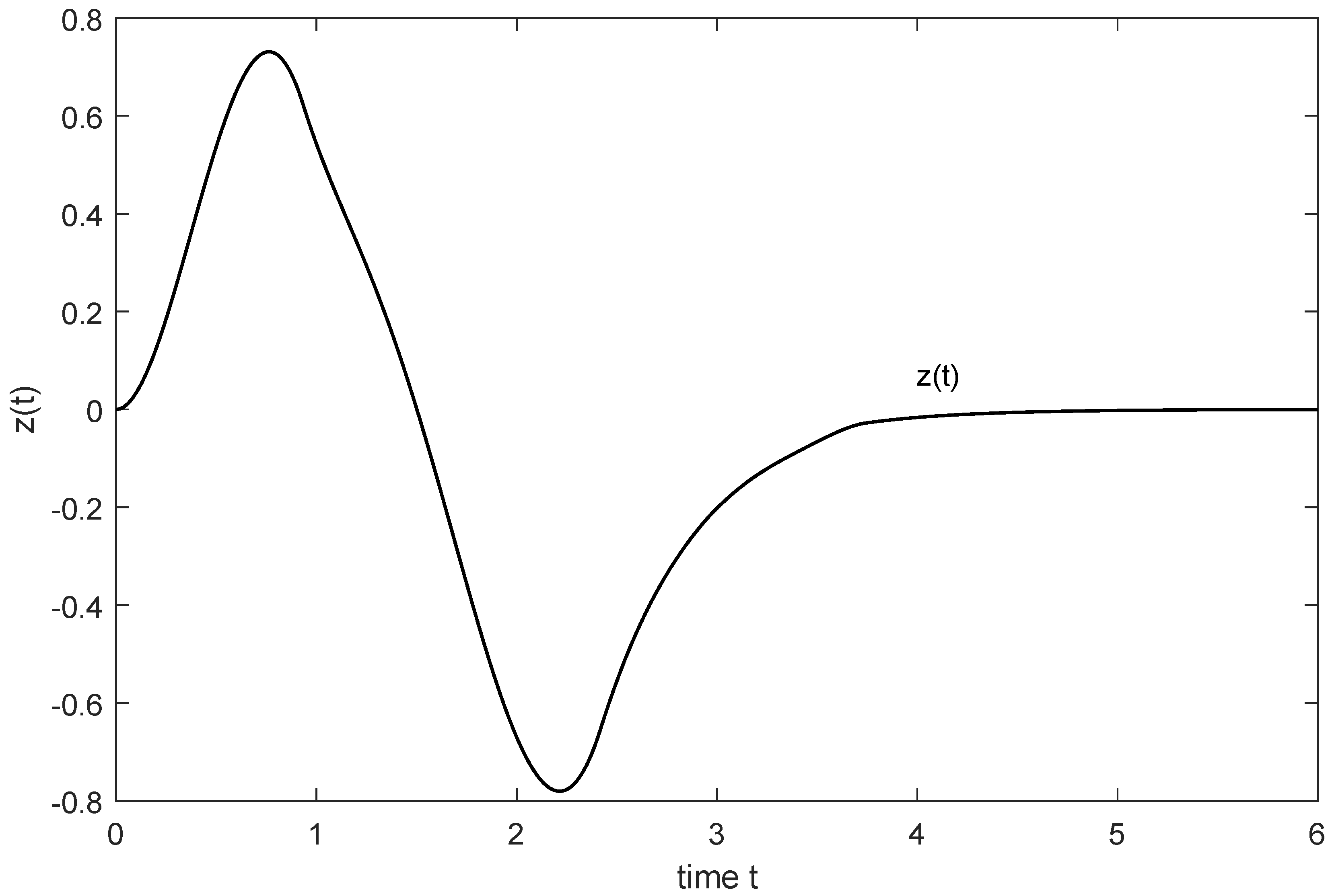
The following numerical example is presented to illustrate the usefulness of the proposed theoretical results.

Example 1.

Consider the system in Equation (1) with the parameter matrices as follows: $E=\left[\begin{array}{cc}1& 0\\ 0& 0\end{array}\right],$ $C=\left[\begin{array}{cc}0.5& 0\\ 0& 0\end{array}\right],$ $A=\left[\begin{array}{cc}-3.45& 0.82\\ 1.35& 1.94\end{array}\right],$ $A_{\tau }=\left[\begin{array}{cc}0.35& 0.12\\ 0.13& 0.15\end{array}\right],$ $B=\left[\begin{array}{c}0.6\\ -0.5\end{array}\right],$ $B_{\omega }=\left[\begin{array}{c}1\\ 1\end{array}\right],$ $D=\left[\begin{array}{cc}1& 0.4\end{array}\right],$ $\Delta B=\left[\begin{array}{c}0\\ 0\end{array}\right],$ $\Delta C=\left[\begin{array}{cc}0.4cos(2t)& 0\\ 0& 0\end{array}\right],$ $\Delta A=\left[\begin{array}{cc}0.3sin(3t)& 0\\ 0& 0.3sin(3t)\end{array}\right],$ $\Delta A_{\tau }=\left[\begin{array}{cc}0.3cos(t)& 0\\ 0& 0.3cos(t)\end{array}\right]$, $\omega (t)=0.3sin(t)$. ${\epsilon }_1=0.16$, ${\epsilon }_2=0.25$, ${\epsilon }_1=0.47$.

Let $\gamma =0.45$. By using Theorem 4 and the Matlab LMI Toolbox, the gain matrices $P,Q,R,L$ can be designed as $P=\left[\begin{array}{cc}13.2741& -0.4528\\ -0.4528& 11.0398\end{array}\right],$ $Q=\left[\begin{array}{cc}16.0723& -0.2634\\ -0.2634& 14.9513\end{array}\right],$ $R=\left[\begin{array}{cc}9.4157& -0.1823\\ -0.1823& 6.0351\end{array}\right],$ $L=\left[\begin{array}{cc}15.1369& -0.3027\\ -3.027& 12.1039\end{array}\right]$.

With the zero-initial condition and the parameters given above, Figure 1 gives the simulations for the trajectory $z(t)$ of the system in Equation (1) under the control law in Theorem 4. Figure 1 demonstrates the effectiveness of the proposed control method.

5. Conclusions

The problem of robust $H_{\infty }$ control for an uncertain singular neutral system is investigated. A new approach is introduced in order to ensure the singular system (Equation $(1)$) is regular and impulse free. On that basis, the matrix equation and an $LMI$ ensure that the system, which is asymptotic and guarantees the $H_{\infty }$ norm bound within $\gamma$ in the closed-loop system for all admissible parameter uncertainties, can be obtained. The needed controller can be constructed by solving the matrix equation and the $LMI$. It should be emphasized that the controller has a generalized inverse form, which is different from the result of [17]. Also, this method can be applied to some practical systems.

References

- Dai, L. Singular Control System; Springer: New York, NY, USA, 1989. [Google Scholar]
- Xia, Y.; Boukas, E.; Shi, P.; Zhang, J. Stability and stabilization of continuous singular hybrid systems. Automatica 2009, 45, 1504–1509. [Google Scholar] [CrossRef]
- Mahmoud, M.S.; Xia, Y.Q. Design of reduced-order l2−l∞ filter design for singular discrete-time systems using strict linear matrix inequalities. IET Control Theory Appl. 2010, 4, 509–519. [Google Scholar] [CrossRef]
- Shen, H.; Su, L.; Park, J.H. Further results on stochastic admissibility for singular Markov jump systems using a dissipative constrained condition. ISA Trans. 2015, 59, 65–71. [Google Scholar] [CrossRef] [PubMed]
- Xu, S.; Dooren, P.; Stefan, R.; Lam, J. Robust stability and stabilization for singular systems with state delay and parameter uncertanity. IEEE Trans. Autom. Control 2002, 47, 1122–1128. [Google Scholar]
- Wei, J. Eigenvalue and stability of singular differential delay systems. J. Math. Anal. Appl. 2004, 297, 305–316. [Google Scholar] [CrossRef] [Green Version]
- Wang, H.; Xue, A.; Lu, R. Absolute stability criteria for a calss of nonlinear singular systems with time delay. Nonlinear Anal. Theory Methods Appl. 2009, 70, 621–630. [Google Scholar] [CrossRef]
- Feng, Y.; Zhu, X.; Zhang, Q. Delay-dependent stability criteria for singular time-delay systems. Acta Autom. Sin. 2010, 36, 433–437. [Google Scholar] [CrossRef]
- Liu, Z.Y.; Lin, C.; Chen, B. A neutral system approach to stability of singular time-delay systems. J. Franklin Inst. 2014, 351, 4939–4948. [Google Scholar] [CrossRef]
- Wang, B.; Yan, J.; Cheng, J.; Zhong, S. New criteria of stability analysis for generalized neural networks subject to time-varying delayed signals. Appl. Math. Comput. 2017, 314, 322–333. [Google Scholar] [CrossRef]
- Choi, H.H.; Chung, M.J. An LMI approach to H∞ controller design for linear time-delay systems. Automatica 1997, 33, 737–739. [Google Scholar] [CrossRef]
- Masubuchi, I.; Kamitane, Y.; Ohara, A.; Suda, N. H∞ control for descriptor systems:a matrix inequality. Automatica 1997, 33, 669–673. [Google Scholar] [CrossRef]
- Liu, H.; Shen, Y.; Zhao, X.D. Delay-dependent observer-based H∞ finite-time control for switched systems with time-varying delay. Nonlinear Anal. Hybrid Syst. 2012, 6, 885–898. [Google Scholar] [CrossRef]
- Kim, J.H. Delay-dependent robust H∞ filtering for uncertain discrete-time singular systems with interval time-varying delay. Automatica 2010, 46, 591–597. [Google Scholar] [CrossRef]
- Kim, J.H. Delay-dependent robust H∞ control for discrete-time uncertain singular systems with interval time-varying delays in state and control input. J. Franklin Inst. 2010, 347, 1704–1722. [Google Scholar] [CrossRef]
- Liu, L.L.; Peng, J.G.; Wu, B.W. H∞ control of singular time-delay systems via discretized Lyapunov functional. J. Franklin Inst. 2011, 348, 749–762. [Google Scholar] [CrossRef]
- Wu, Z.G.; Park, J.H.; Su, H.; Song, B.; Chu, J. Mixed H∞ and passive filtering for singular systems with time delays. Signal Process. 2013, 93, 1705–1711. [Google Scholar] [CrossRef]
- Mei, F. Delay-dependent robust H∞ control for uncertain singular systems with state delay. Acta Autom. Sin. 2009, 35, 65–70. [Google Scholar]
- Wu, Z.; Su, H.; Chu, J. Improved results on delay-dependent H∞ control for singular time-delay systems. Acta Autom. Sin. 2009, 35, 1101–1106. [Google Scholar] [CrossRef]
- Fridman, E.; Shaked, U. H∞ control of linear state-delay descriptor systems:an LMI approach. Linear Algebra Its Appl. 2002, 351, 271–302. [Google Scholar] [CrossRef]
- Lee, J.H.; Kim, S.W.; Kwon, W.H. Memoryless H∞ controller for state delayed systems. IEEE Trans. Autom. Control 1994, 39, 159–162. [Google Scholar]
- Huang, S.S.; Lee, T.T. Memoryless H∞ controller for singular systems with delayed state and control. J. Franklin Inst. 1999, 336, 911–923. [Google Scholar] [CrossRef]
- Kim, J.H. New design method on memoryless H∞ control for singular systems with delayed state and control using LMI. J. Franklin Inst. 2005, 342, 321–327. [Google Scholar] [CrossRef]
- Ji, X.F.; Su, H.Y.; Chu, J. An LMI approach to robust H∞ control for uncertain singular time-delay systems. J. Control Theory Appl. 2006, 4, 361–366. [Google Scholar] [CrossRef]
- Guan, X.; Chen, C.; Peng, H.; Fan, Z. Time-delayed feedback control of time-delay chaotic systems. Int. J. Bifurc. Chaos 2003, 13, 193–205. [Google Scholar] [CrossRef]
- Hale, J.K.; Lunel, S.M.V. Introduction to Functional Differential Equations; Springer Science & Business Media: Berlin/Heidelberg, Germany, 2013. [Google Scholar]
- Boyd, S.; Ghaoui, L.E.; Feron, E. Linear Matrix Inequalities in System and Control Theory; Society for Industrial and Applied Mathematics: Philadelphia, PA, USA, 1994. [Google Scholar]
- Mahmoud, M. Robust Control and Filtering for Time-Delay Systems; Control Engineering Series; Marcel Dekker: New York, NY, USA, 2000. [Google Scholar]
- Wang, G.; Wei, Y.; Qiao, S.; Lin, P.; Chen, Y. Generalized Inverses: Theorey and Computations; Science Press: Beijing, China, 2004. [Google Scholar]
Figure 1.
The trajectory of of the system in Equation (1).
© 2019 by the authors. Licensee MDPI, Basel, Switzerland. This article is an open access article distributed under the terms and conditions of the Creative Commons Attribution (CC BY) license (http://creativecommons.org/licenses/by/4.0/).
Share and Cite
MDPI and ACS Style
Huo, Y.; Liu, J.-B. Robust H∞ Control For Uncertain Singular Neutral Time-Delay Systems. Mathematics 2019, 7, 217. https://doi.org/10.3390/math7030217
AMA Style
Huo Y, Liu J-B. Robust H∞ Control For Uncertain Singular Neutral Time-Delay Systems. Mathematics. 2019; 7(3):217. https://doi.org/10.3390/math7030217
Chicago/Turabian StyleHuo, Yuhong, and Jia-Bao Liu. 2019. "Robust H∞ Control For Uncertain Singular Neutral Time-Delay Systems" Mathematics 7, no. 3: 217. https://doi.org/10.3390/math7030217
Note that from the first issue of 2016, this journal uses article numbers instead of page numbers. See further details here.