SRIFA: Stochastic Ranking with Improved-Firefly-Algorithm for Constrained Optimization Engineering Design Problems


Department of CSE, Visvesvaraya National Institute of Technology, Nagpur 440010, India
*
Author to whom correspondence should be addressed.
Mathematics 2019, 7(3), 250; https://doi.org/10.3390/math7030250
Submission received: 2 February 2019
/
Revised: 1 March 2019
/
Accepted: 5 March 2019
/
Published: 11 March 2019
(This article belongs to the Special Issue Evolutionary Computation)
Abstract
:Firefly-Algorithm (FA) is an eminent nature-inspired swarm-based technique for solving numerous real world global optimization problems. This paper presents an overview of the constraint handling techniques. It also includes a hybrid algorithm, namely the Stochastic Ranking with Improved Firefly Algorithm (SRIFA) for solving constrained real-world engineering optimization problems. The stochastic ranking approach is broadly used to maintain balance between penalty and fitness functions. FA is extensively used due to its faster convergence than other metaheuristic algorithms. The basic FA is modified by incorporating opposite-based learning and random-scale factor to improve the diversity and performance. Furthermore, SRIFA uses feasibility based rules to maintain balance between penalty and objective functions. SRIFA is experimented to optimize 24 CEC 2006 standard functions and five well-known engineering constrained-optimization design problems from the literature to evaluate and analyze the effectiveness of SRIFA. It can be seen that the overall computational results of SRIFA are better than those of the basic FA. Statistical outcomes of the SRIFA are significantly superior compared to the other evolutionary algorithms and engineering design problems in its performance, quality and efficiency.
1. Introduction
Nature-Inspired Algorithms (NIAs) are very popular in solving real-life optimization problems. Hence, designing an efficient NIA is rapidly developing as an interesting research area. The combination of evolutionary algorithms (EAs) and swarm intelligence (SI) algorithms are commonly known as NIAs. The use of NIAs is popular and efficient in solving optimization problems in the research field [1]. EAs are inspired by Darwinian theory. The most popular EAs are genetic algorithm [2], evolutionary programming [3], evolutionary strategies [4], and genetic programming [5]. The term SI was coined by Gerardo Beni [6], as it mimics behavior of biological agents such as birds, fish, bees, and so on. Most popular SI algorithms are particle swarm optimization [7], firefly algorithm [8], ant colony optimization [9], cuckoo search [10] and bat algorithm [11]. Recently, many new population-based algorithms have been developed to solve various complex optimization problem such as killer whale algorithm [12], water evaporation algorithm [13], crow search algorithm [14] and so on. The No-Free-Lunch (NFL) theorem described that there is not a single appropriate NIA to solve all optimization problems. Consequently, choosing a relevant NIAs for a particular optimization problem involves a lot of trial and error. Hence, many NIAs are studied and modified to make them more powerful with regard to efficiency and convergence rate for some optimization problems. The primary factor of NIAs are intensification (exploitation) and diversification (exploration) [15]. Exploitation refers to finding a good solution in local search regions, whereas exploration refers to exploring global search space to generate diverse solutions [16].
Optimization algorithms can be classified in different ways. NIAs can be simply divided into two types: stochastic and deterministic [17]. Stochastic (in particular, metaheuristic) algorithms always have some randomness. For example, the firefly algorithm has “” as a randomness parameter. This approach provides a probabilistic guarantee for a faster convergence of global optimization problem, usually to find a global minimum or maximum at an infinite time. In the deterministic approach, it ensures that, after a finite time, the global optimal solution will be found. This approach follows a detailed procedure and the path and values of both dimensions of problem and function are reputable. Hill-climbing is a good example of deterministic algorithm, and it follows same path (starting point and ending point) whenever the program is executed [18].
Real-world engineering optimization problems contain a number of equality and inequality constraints, which alter the search space. These problems are termed as Constrained-Optimization Problems (COPs). The minimization COPs defined as:
where is the objective-function given in Equation (1), n-dimensional design variables, and are the lower and upper bounds, inequality with m constraints and equality with constraints.
The feasible search space is represented as the equality (q) and inequality (m). Some point in the contains feasible or infeasible solutions. The active constraint is defined as inequality constraints that are satisfied when at given point . In feasible regions, all constraints (i.e., equality constraints) were acknowledged as active constraints at all points.
In NIA problems, most of the constraint-handling techniques deal with inequality constraints. Hence, we have transformed equality constrained into equality using some tolerance value ():
where and ’’ is tolerance allowed. Apply the value of tolerance for equality constraints for a given optimization problem. Then, the constraint-violation of an individual from the constraint can be calculated by
The maximum constraint-violation of of every constraint in the all individual or population is given as:
With this background, the rest of paper is ordered as follows: Section 2 explains the classification of constrained-Handling Techniques (CHT); Section 3 deals with an overview of Constrained FA; Section 4 gives the outline of SR and OBL approaches. Section 5 described the proposed SRIFA with OBL; the experimental setup and computational outcomes of the SRIFA with 24 CEC 2006 benchmark test functions are illustrated in Section 6. The comparison of SRIFA with existing metaheuristic algorithms is also discussed with respect to its performance and effectiveness. The computational results of the SRIFA are examined with an engineering design problem in Section 7. Finally, in Section 8, conclusions of the paper are given.
2. Constrained-Handling Techniques (CHT)
Classification of CHT
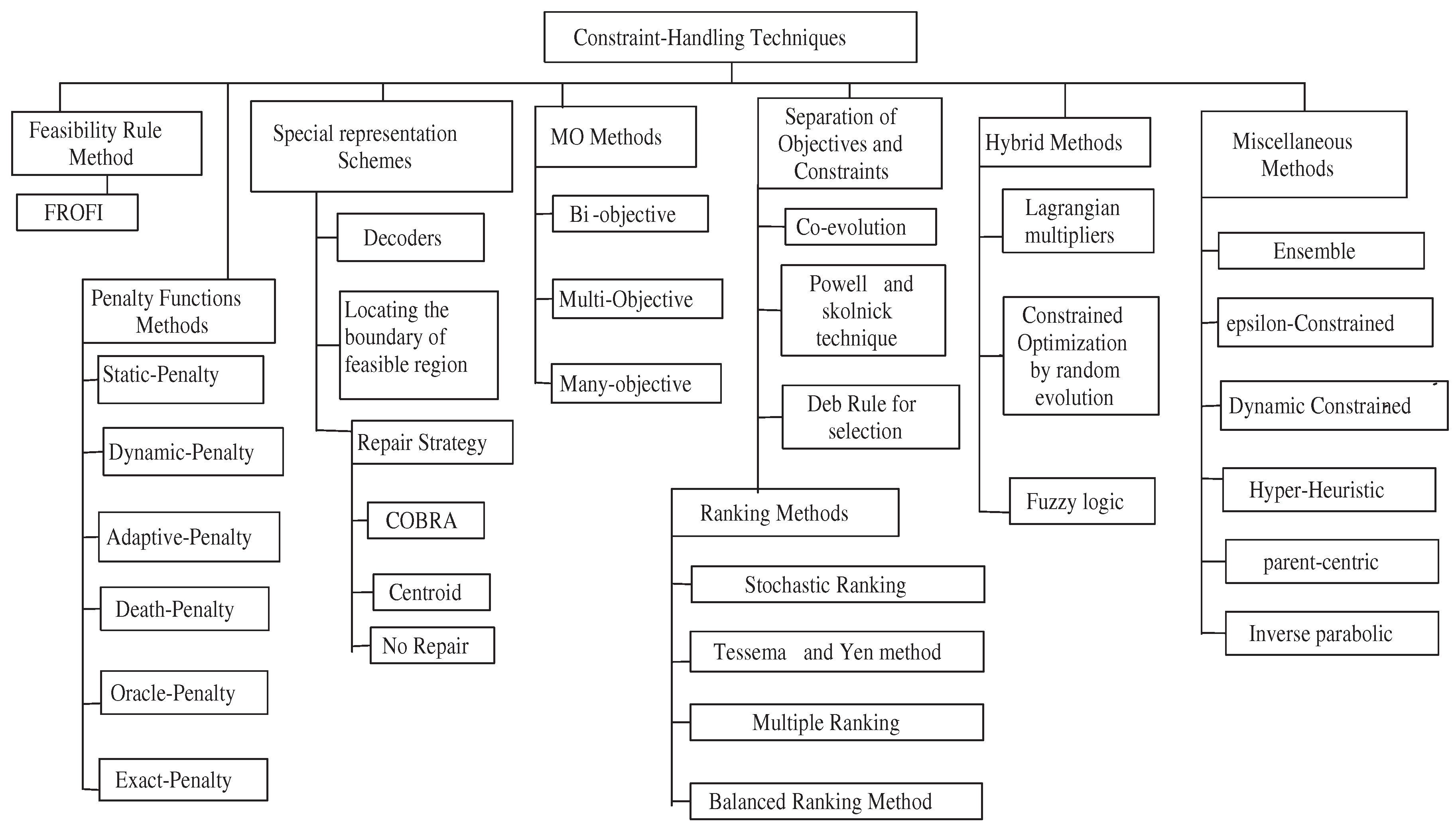
In this section, we provide a literature survey of various CHT approaches that are adapted into NIAs to solve COPs. The classification of constrained handling approaches is shown in Figure 1. In the past few decades, various CHTs have been developed, particularly for EAs. Mezura-Montes and Coello conducted a comprehensive survey of NIA [19].
- Feasibility Rules Approach: The most effective CHT was proposed by Deb [20]. Between any two solutions and compared, is better than , under the following conditions:
- (a)
- If is a feasible solution, then solution is not.
- (b)
- Between two and feasible solutions, if has better objective value over , then is preferred.
- (c)
- Between two and infeasible solutions, if has the lowest sum of constraint-violation over , then is preferred.
Wang and Li [21] integrated a Feasibility-Rule integrated with Objective Function Information (FROFI), where Differential Evolution (DE) is used as a search algorithm along with feasibility rule. - Multi-objective Methods (MO) or Vector optimization or Pareto-optimization: It is an optimization problems that has two or more objectives [28]. There are roughly two types of MO methods: bi-objective and many-objective.
- Split-up objective and constraints: There are many techniques to handle split-up objective and constraints. These techniques are co-evolution, Powell and Skolnick technique, Deb-rule and ranking method. There are different types of ranking methods such as stochastic ranking, Tessema and Yen method, multiple ranking and the balanced ranking method.
- Hybrid Method: The NIAs combined with a classical constrained method or heuristic method are called as hybrid methods. The hybrid method includes Lagrangian multipliers, constrained Optimization by random evolution and fuzzy logic [25].
3. Overview of Constrained FA
3.1. Basic FA
FA is a swarm-based NIAs proposed by Xin-she Yang [8]. Fister et al. [32] carried out in detail comprehensive review of FA. The basic FA pseudo-code is indicated in Algorithm 1. The mathematical formulation of the basic FA is as follows (Figure 2):
Let us consider that attractiveness of FA is assumed as brightness (i.e., fitness function). The distance between brightness of two fireflies (assume u and v) is given as:
where I is an intensity of light-source parameter, is an absorption coefficient, and is distance between two fireflies u and v. is the intensity of light source parameter when r = 0. The attractiveness for two fireflies u and v (u is more attractive than v) is defined as:
is attractiveness parameter when r = 0.
Movement of fireflies are basically based on the attractiveness, when a firefly u is less attractive than firefly v; then, firefly u moves towards firefly v and it is determined by Equation (10):
where the second term is an attractive parameter, the third term is a randomness parameter and is a vector of random-numbers generated uniform distribution between 0 and 1.
3.2. Constrained FA
The FA Combined with CHT has been widely used for solving COPs. Some typical constrained FA (CFA) has been briefly discussed below.
To solve engineering optimization problems, the adaptive-FA is designed has been discussed in [33]. Costa et al. [34] used penalty based techniques to evaluate different test functions for global optimization with FA. Brajevic et al. [35] developed feasibility-rule based with FA for COPs. Kulkarni et al. [36] proposed a modified feasibility-rule based for solving COPs using probability. The upgraded FA (UFA) is proposed to solve mechanical engineering optimization problem [37]. Chou and Ngo designed a multidimensional optimization structure with modified FA (MFA) [38].
| Algorithm 1 Stochastic Ranking Approach (SRA) |
| 1: Number of population (N), balanced dominance of two solution of , is sum of constrained violation, m is individual who will be ranked 2: Rank the individual based on and 3: Calculate = 1, */ and is variable of f(z) 4: for i = 1 to n do 5: for k = 1 to m-1 do 6: Random R = U(0, 1) */random number generator 7: end for 8: if ((() = (() = 0)) or R < then 9: if (f() > f()) then 10: swap (,) 11: end if 12: else if ( > ) then 13: swap (, ) end if 14: end if 15: if no swapping then break; 16: end if 17: end for |
4. Stochastic Ranking and Opposite-Based Learning (OBL)
This section represents an overview of SR and OBL.
4.1. Stochastic Ranking Approach (SRA)
This approach, which was introduced by Runarsson and Yao [39], which balances fitness or (objective function) and dominance of a penalty approach. Based on this, the SRA uses a simple bubble sort technique to rank the individuals. To rank the individual in SRM, is introduced, which is used to compare the fitness function in infeasible area of search space. Normally, when we take any two individuals for comparison, three possible solutions are formed.
(a) if both individuals are in a feasible region, then the smallest fitness function is given the highest priority; (b) For both individuals at an infeasible region, an individual having smallest constraint-violation () is preferred to fitness function and is given the highest priority; and (c) if one individual is feasible and other is infeasible, then the feasible region individual is given highest priority. The pseudo code of SRM is given in Algorithm 1.
4.2. Opposition-Based Learning (OBL)
The OBL is suggested by Tizhoosh in the research industry, which is inspired by a relationship among the candidate and its opposite solution. The main aim of the OBL is to achieve an optimal solution for a fitness function and enhance the performance of the algorithm [40]. Let us assume that z∈ [] is any real number, and the opposite solution of z is denoted as and defined as
Let us assume that is an n-dimensional decision vector, in which ∈ and . In the opposite vector, p is defined as where .
5. The Proposed Algorithm
The most important factor in NIAs is to maintain diversity of population in search space to avoid premature convergence. From the intensification and diversification viewpoints, an expansion in diversity of population revealed that NIAs are in the phase of intensification, while a decreased population of diversity revealed that NIAs are in the phase of diversification. The adequate balance between exploration and exploitation is achieved by maintaining a diverse populations. To maintain balance between intensification and diversification, different approaches were proposed such as diversity maintenance, diversity learning, diversity control and direct approaches [16]. The diversity maintenance can be performed using a varying size population, duplication removal and selection of a randomness parameter.
On the other hand, when the basic FA algorithm is performed with insufficient diversification (exploration), it leads to a solution stuck in local optima or a suboptimal region. By considering these issues, a new hybridizing algorithm is proposed by improving basic FA.
5.1. Varying Size of Population
A very common and simple technique is to increase the population size in NIAs to maintain the diversity of population. However, due to an increase in population size, computation time required for the execution of NIAs is also increased. To overcome this problem, the OBL concept is applied to improve the efficiency and performance of basic FA at the initialization phase.
5.2. Improved FA with OBL
In the population-based algorithms, premature convergence in local optimum is a common problem. In the basic FA, every firefly moves randomly towards the brighter one. In that condition, population diversity is high. After some generation, the population diversity decreases due to a lack of selection pressure and this leads to a trap solution at local optima. The diversification of FA is reduced due to premature convergence. To overcome this problem, the OBL is applied to an initial phase of FA, in order to increase the diversity of firefly individuals.
In the proposed Improved Firefly Algorithm (IFA), we have to balance intensification and diversification for better performance and efficiency of the proposed FA. To perform exploration, a randomization parameter is used to overcome local optimum and to explore global search. To balance between intensification and diversification, the random-scale factor (R) was applied to generate randomly populations. Das et al. [41] used a similar approach in DE:
where is a vth parameter of the uth firefly, is upper-bound, is a lower-bound of vth value and rand (0, 1) is randomly distributed of the random-number.
The movement of fireflies using Equation (10) will be modified as
5.3. Stochastic Ranking with an Improved Firefly Algorithm (SRIFA)
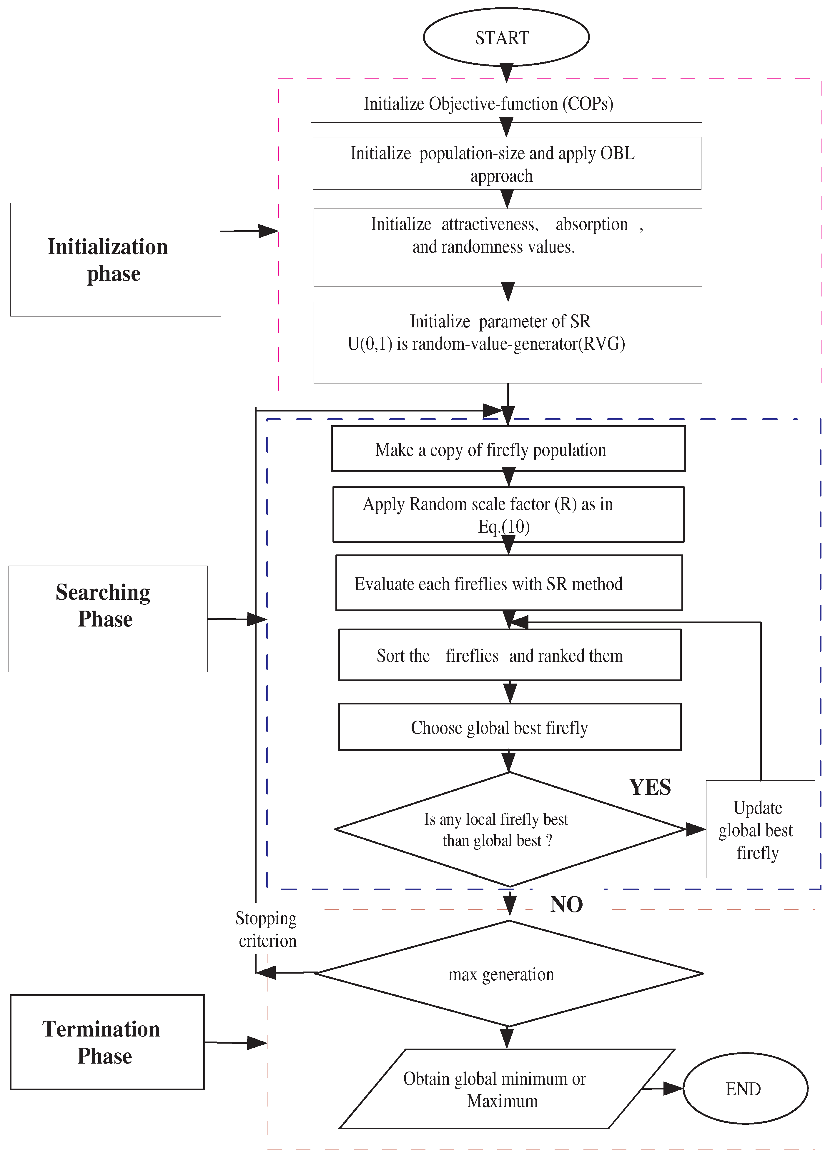
Many studies are published in literature for solving COPs using EAs and FA. However, it is quite challenging to apply this approach for constraints effectively handling optimization problems. FA produces admirable outcomes on COPs and it is well-known for having a quick convergence rate [42]. As a result of the quick convergence rate of FA and popularity of the stochastic-ranking for CHT, we proposed a hybridized technique for constrained optimization problems, known as Stochastic Ranking with an Improved Firefly Algorithm (SRIFA). The flowchart of SRIFA is shown in Figure 3.
5.4. Duplicate Removal in SRIFA
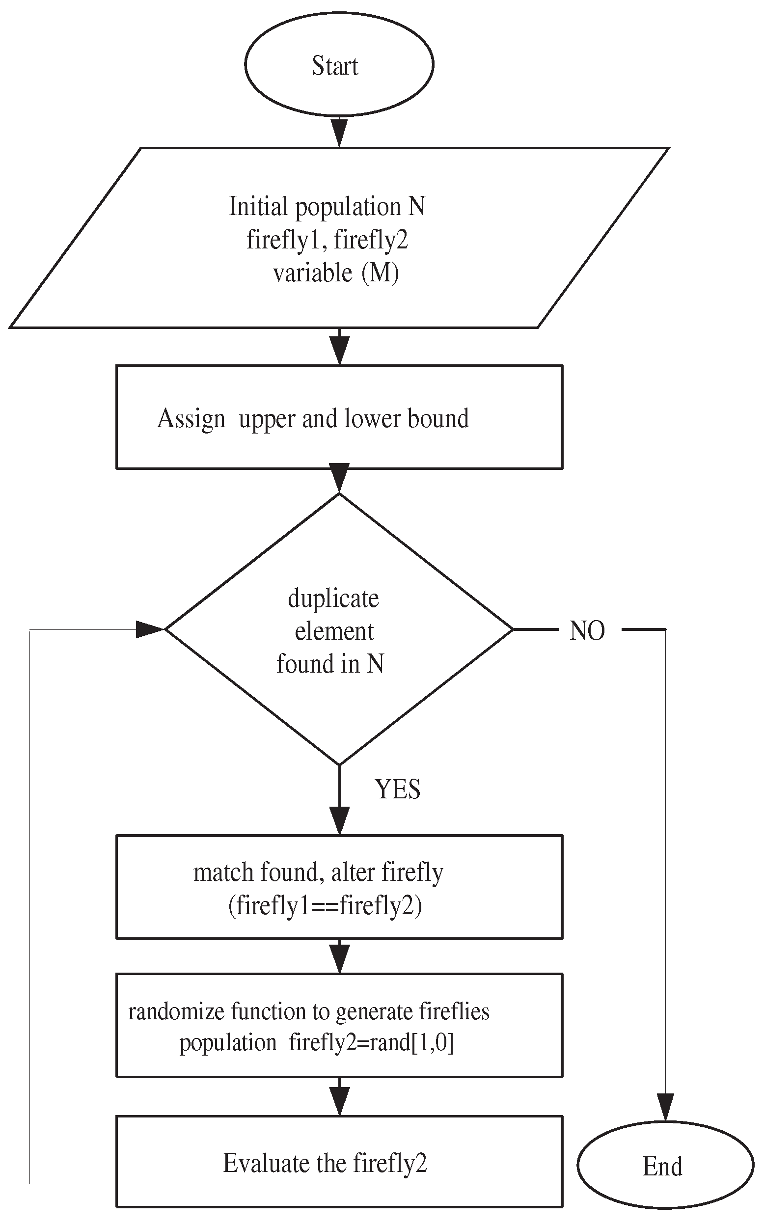
The duplicate individuals in a population should be eliminated and new individuals should generated and inserted randomly into SRIFA. Figure 4 represents the duplication removal in SRIFA.
6. Experimental Results and Discussions
To examine the performance of SRIFA with existing NIAs, the proposed algorithm is applied to 24 numerical benchmark test functions given in CEC 2006 [43]. This preferred benchmark functions have been thoroughly studied before by various authors.
In Table 1, the main characteristics of 24 test function are determined, where a fitness function (f(z)), number of variables or dimensions (D), is expressed as a feasibility ratio between a feasible solution (Feas) with search region (SeaR), Linear-Inequality constraint (LI), Nonlinear Inequality constraint (NI), Linear-Equality constraint (LE), Nonlinear Equality constraint (NE), number active constraint represented as () and an optimal solution of fitness function denoted (OPT) are given. For convenience, all equality constraints, i.e., are transformed into inequality constraint , where is a tolerance value, and its goal is to achieve a feasible solution [43].
6.1. Experimental Design
To investigate the performance and effectiveness of the SRIFA, it is tested over 24 standard- functions and five well-known engineering design-problems. All experiments of COPs were experimented on an Intel core (TM) processor @3.40 GHz with 8 GB RAM memory, where an SRIFA algorithm was programmed with Matlab 8.4 (R2014b) under Win7 (x64). Table 2 shows the parameter used to conduct computational experiments of SRIFA algorithms. For all experiments, 30 independent runs were performed for each problem. To investigate efficiency and effectiveness of the SRIFA, various statistical parameters were used such as best, worst, mean, global optimum and standard-deviation (Std). Results in bold indicate best results obtained.
6.2. Calibration of SRIFA Parameters
In this section, we have to calibrate the parameter of the SRIFA. According to the strategy of the SRIFA, described in Figure 2, the SRIFA contains eight parameters: size of population (), initial randomization value (), initial attractiveness value (), absorption-coefficient (), max-generation (G), total number of function evaluations (), probability and varphi (). To derive a suitable parameter, we have performed details of fine-tuning by varying parameters of SRIFA. The choice of each of these parameters as follows: ()∈ (5 to 100 with an interval of 5), () ∈ (0.10 to 1.00 with an interval of 0.10), () ∈ (0.10 to 1.00 with an interval 0.10), () ∈ (0.01 to 100 with an interval of 0.01 until 1 further 5 to 100), (G) ∈ (1000 to 10,000 with an interval of 1000), ∈ (1000 to 240,000), = ∈ (0.1 to 0.9 with an interval of 0.1) and () ∈ (0.1 to 1.0 with an interval of 0.1). The best optimal solutions obtained by SRIFA parameter experiments from the various test functions. In Table 2, the best parameter value for experiments for the SRIFA are described.
6.3. Experimental Results of SRIFA Using a GKLS (GAVIANO, KVASOV, LERA and SERGEYEV) Generator
In this experiment, we have compared the proposed SRIFA with two novel approaches: Operational Characteristic and Aggregated Operational Zone. An operational characteristic approach is used for comparing deterministic algorithms, whereas an aggregated operational zone approach is used by extending the idea of operational characteristics to compare metaheuristic algorithms.
The proposed algorithm is compared with some widely used NIAs (such as DE, PSO and FA) and the well-known deterministic algorithms such as DIRECT, DIRECT-L (locally-biased version), and ADC (adaptive diagonal curves). The GKLS test classes generator is used in our experiments. The generator allows us to randomly generate 100 test instances having local minima and dimension. In this experiment, eight classes (small and hard) are used (with dimensions of n = 2, 3, 4 and 5) [45]. The control parameters of the GKLS-generator required for each class contain 100 functions and are defined by the following parameters: design variable or problem dimension (N), radius of the convergence region (), distance from of the paraboloid vertex and global minimum (r) and tolerance (). The value of control parameters are given in Table 3.
From Table 4, we can see that the mean value of generations required for computation of 100 instances are calculated for each deterministic and metaheuristic algorithms using an GKLS generator. The values “>m(i)” indicate that the given algorithm did not solve a global optimization problem i times in 100 × 100 instances (i.e., 1000 runs for deterministic and 10,000 runs for metaheuristic algorithms). The maximum number of generations is set to be . The mean value of generation required for proposed algorithm is less than other algorithms, indicating that the performance SRIFA is better than the given deterministic and metaheuristic algorithms.
6.4. Experimental Results FA and SRIFA
In our computational experiment, the proposed SRIFA is compared with the basic FA. It differs from the basic FA in following few points. In the SRIFA, the OBL technique is used to enhance initial population of algorithm, while, in FA, fixed generation is used to search for optimal solutions. In the SRIFA, the chaotic map (or logistic map) is used to improve absorption coefficient , while, in the FA, fixed iteration is applied to explore the global solution. The random scale factor (R) was used to enhance performance in SRIFA. In addition, SRIFA uses Deb’s rules in the form of the stochastic ranking method.
The experimental results of the SRIFA with basic FA are shown in Table 5. The comparison between SRIFA and FA are conducted using 24 CEC (Congress on Evolutionary-Computation) benchmark test functions [43]. The global optimum, CEC 2006 functions, best, worst, mean and standard deviation (Std) outcomes produced by SRIFA and FA in over 25 runs are described in Table 5.
In Table 5, it is clearly observed that SRIFA provides promising results compared to the basic FA for all benchmark test functions. The proposed algorithm found optimal or best solutions on all test functions over 25 runs. For two functions (G20 and G22), we were unable to find any optimal solution. It should be noted that ’N-F’ refers to no feasible result found.
6.5. Comparison of SRIFA with Other NIAs
To investigate the performance and effectiveness of the SRIFA, these results are compared with five metaheuristic algorithms. These algorithms are stochastic ranking with a particle-swarm-optimization (SRPSO) [46], self adaptive mix of particle-swarm-optimization (SAMO-PSO) [47], upgraded firefly algorithm (UFA) [37], an ensemble of constraint handling techniques for evolutionary-programming (ECHT-EP2) [48] and a novel differential-evolution algorithm (NDE) [49]. To evaluate proper comparisons of these algorithms, the same number of function evaluations (NFEs = 240,000) were chosen.
The statistical outcomes achieved by SRPSO, SAMO-PSO, UFA, ECHT-EP2 and NDE for 24 standard functions are listed in Table 6. The outcomes given in bold letter indicates best or optimal solution. N-A denotes “Not Available”. The benchmark function G20 and G22 are discarded from the analysis, due to no feasible results were obtained.
On comparing SRIFA with SRPSO for 22 functions as described in Table 6, it is clearly seen that, for all test functions, statistical outcomes indicate better performance in most cases. The SRIFA obtained the best or the same optimal values among five metaheuristic algorithms. In terms of mean outcomes, SRIFA shows better outcomes to test functions G02, G14, G17, G21 and G23 for all four metaheuristic algorithms (i.e., SAMO-PSO, ECHT-EP2, UFA and NDE). SRIFA obtained worse mean outcomes to test function G19 than NDE. In the rest of all test functions, SRIFA was superior to all compared metaheuristic algorithms.
6.6. Statistical Analysis with Wilcoxon’s and Friedman Test
Statistical analysis can be classified as parametric and non-parametric test (also known as distribution-free tests). In parametric tests, some assumptions are made about data parameters, while, in non-parametric tests, no assumptions are made for data parameters. We performed statistical analysis of data by non-parametric tests. It mainly consists of a Wilcoxon test (pair-wise comparison) and Friedman test (multiple comparisons) [50].
The outcomes of statistical analysis after conducting a Wilcoxon-test between SRIFA and the other five metaheuristic algorithms are shown in Table 7. The value indicates that the first algorithm is significantly superior than the second algorithm, whereas indicates that the second algorithm performs better than the first algorithm. In Table 7, it is observed that values are higher than values in all cases. Thus, we can conclude that SRIFA significantly outperforms compared to all metaheuristic algorithms.
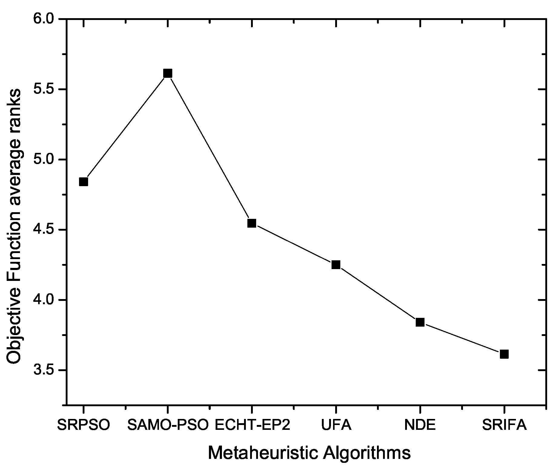
The statistical analysis outcomes by applying Friedman test are shown in Table 8. We have ranked the given metaheuristic algorithms corresponding to their mean value. From Table 8, SRIFA obtained first ranking (i.e., the lowest value gets the first rank) compared to all metaheuristic algorithms over the 22 test functions. The average ranking of the SRIFA algorithm based on the Friedman test is described in Figure 5.
6.7. Computational Complexity of SRIFA
In order to reduce complexity of the given problem, constraints are normalized. Let n be population size and t is iteration. Generally in NIAs, at each iteration, a complexity is , where is the maximum amount of function evaluations allowed and and is the cost of objective function. At the initialization phase of SRIFA, the computational complexity of population generated randomly by the OBL technique is . In a searching and termination phase, the computational complexity of two inner loops of FA and stochastic ranking using a bubble sort are +. The total computational complexity of SRIFA is = + +≈.
7. SRIFA for Constrained Engineering Design Problems
In this section, we evaluate the efficiency and performance of SRIFA by solving five widely used constrained engineering design problems. These problems are: (i) tension or compression spring design [51]; (ii) welded-beam problem [52]; (iii) pressure-vessel problem [53]; (iv) three-bar truss problem [51]; and (v) speed-reducer problem [53]. For every engineering design problem, statistical outcomes were calculated by executing 25 independent runs for each problem. The mathematical formulation of all five constrained engineering design problems are given in “Appendix A”.
Every engineering problem has unique characteristics. The best value of constraints, parameter and objective values obtained by SRIFA for all five engineering problems are listed in Table 9. The statistical outcomes and number of function-evaluations (NFEs) of SRIFA for all five engineering design problems are listed in Table 10. These results were obtained by SRIFA over 25 independent runs.
7.1. Tension/Compression Spring Design
A tension/compression spring-design problem is formulated to minimize weight with respect to four constraints. These four constraints are shear stress, deflection, surge frequency and outside diameter. There are three design variables, namely: mean coil (D), wire-diameter d and the amount of active-coils N.
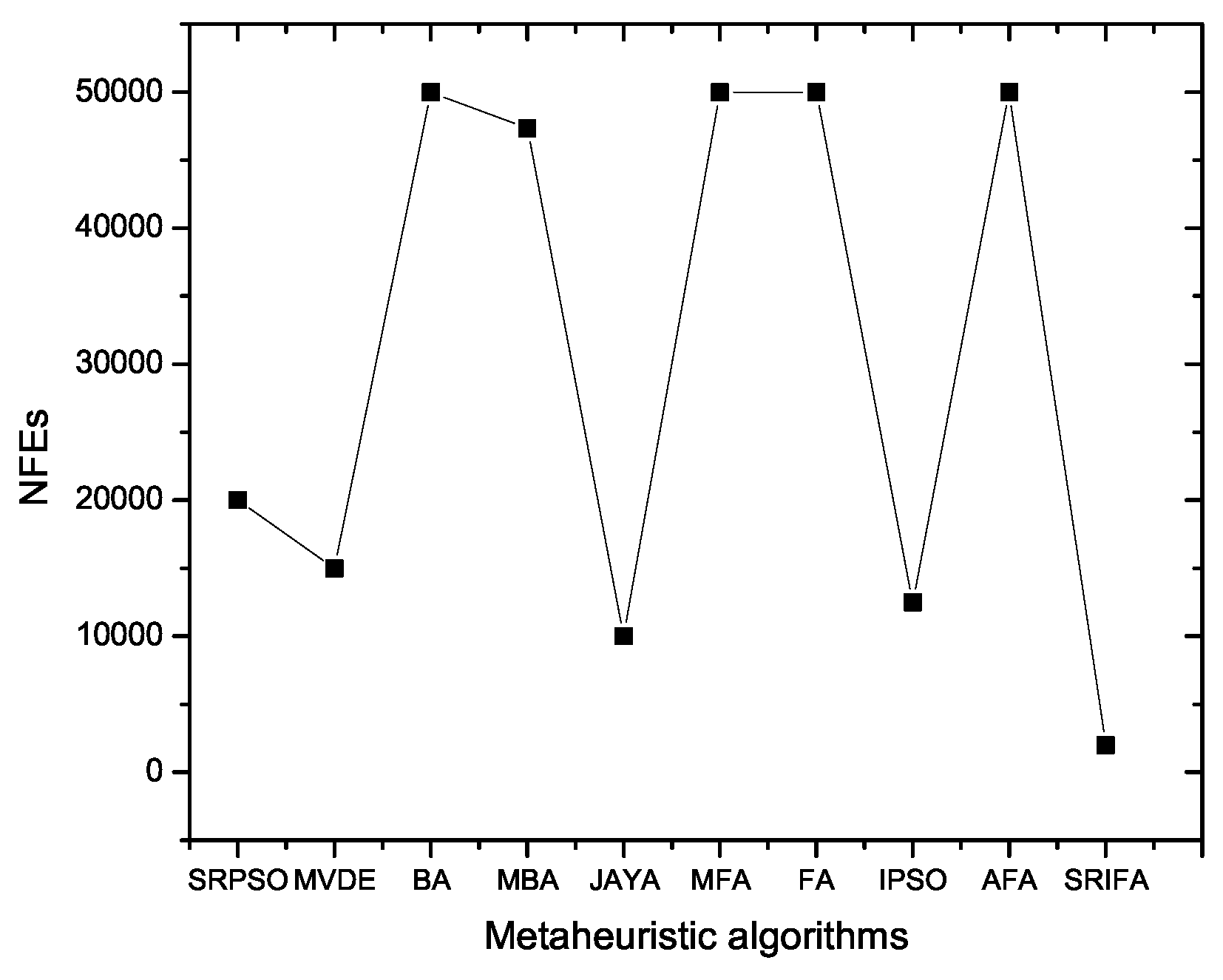
This proposed SRIFA approach is compared to SRPSO [46], MVDE [54], BA [44], MBA [55], JAYA [56], PVS [57], UABC [58], IPSO [59] and AFA [33]. The comparative results obtained by SRIFA for nine NIAs are given in Table 11. It is clearly observed that SRIFA provides the most optimum results over nine metaheuristic algorithms. The mean, worst and SD values obtained by SRIFA are superior to those for other algorithms. Hence, we can draw conclusions that SRIFA performs better in terms of statistical values. The comparison of the number of function evacuations (NFEs) with various NIAs is plotted in Figure 6.
7.2. Welded-Beam Problem
The main objective of the welded-beam problem is to minimize fabrication costs with respect to seven constraints. These constraints are bending stress in the beam ( ), shear stress ( ), deflection of beam ( ), buckling load on the bar (), side constraints, weld thickness and member thickness (L).
Attempts have been made by many researchers to solve the welded-beam-design problem. The SRIFA was compared with SRPSO, MVDE, BA, MBA, JAYA, MFA, FA, IPSO and AFA. The statistical results obtained by SRIFA on comparing with nine metaheuristic algorithms are described in Table 12. It can be seen that statistical results obtained from SRIFA performs better than all metaheuristic algorithms.
The results obtained by the best optimum value for SRIFA performs superior to almost all of the seven algorithms (i.e., SRPSO, MVDE, BA, MBA, MFA, FA, and IPSO) but almost the same optimum value for JAYA and AFA. In terms of mean results obtained by SRIFA, it performs better than all metaheuristic algorithms except AFA as it contains the same optimum mean value. The standard deviation (SD) obtained by SRIFA is slightly worse than the SD obtained by MBA. From Table 12, it can be seen that SRIFA is superior in terms of SD for all remaining algorithms. The smallest NFE result is obtained by SRIFA as compared to all of the metaheuristic algorithms. The comparisons of NFEs with all NIAs are shown in Figure 7.
7.3. Pressure-Vessel Problem
The main purpose of the pressure-vessel problem is to minimize the manufacturing cost of a cylindrical-vessel with respect to four constraints. These four constraints are thickness of head (), thickness of pressure vessel (), length of vessel without head (L) and inner radius of the vessel (R).
The SRIFA is optimized with SRPSO, MVDE, BA, EBA [60], FA [44], PVS, UABC, IPSO and AFA. The statistical results obtained by SRIFA for nine metaheuristic algorithms are listed in Table 13. It is clearly seen that SRIFA has the same best optimum value when compared to six algorithms (MVDE, BA, EBA, PVS, UABC and IPSO). The mean, worst, SD and NFE results obtained by SRIFA are superior to all NIAs. The comparisons of NFEs with all NIAs are shown in Figure 8.
7.4. Three-Bar-Truss Problem
The main purpose of the given three-bar-truss problem is to minimize the volume of a three-bar truss with respect to three stress constraints.
The SRIFA is compared with SRPSO, MVDE, NDE [49], MAL-FA [61], UABC, WCA [62] and UFA. The statistical results obtained by SRIFA in comparison with the seven NIAs are described in Table 14. It is clearly seen that SRIFA has almost the same best optimum value except with the UABC algorithm. In terms of mean and worst results obtained, SRIFA performed better compared to all metaheuristic algorithms except NDE and UFA, which contain the same optimum mean and worst value. The standard deviation (SD) obtained by SRIFA is superior to all metaheuristic algorithms. The smallest NFE value is obtained by SRIFA compared to all other metaheuristic algorithms. The comparisons of NFEs with all other NIAs are shown in Figure 9.
7.5. Speed-Reducer Problem
The goal of the given problem is to minimize the speed-reducer of weight with respect to eleven constraints. This problem has seven design variables that are gear face, number of teeth in pinion, teeth module, length of first shaft between bearings. diameter of first shaft, length of second shaft between bearings, and diameter of second shaft.
The proposed SRIFA approach is compared with SRPSO, MVDE, NDE, MBA, JAYA, MBA, UABC, PVS, IPSO and AFA. The statistical results obtained by SRIFA for nine metaheuristic algorithms are listed in Table 15. It can be observed that the SRIFA provides the best optimum value among all eight metaheuristic algorithms except JAYA (they have the same optimum value). The statistical results (best, mean and worst) value obtained by SRIFA and JAYA algorithm is almost the same, while SRIFA requires less NFEs for executing the algorithm. Hence, we can conclude that SRIFA performed better in terms of statistical values. Comparisons of number of function evacuations (NFEs) with various metaheuristic algorithm are plotted in Figure 10.
8. Conclusions
This paper proposes a review of constrained handling techniques and a new hybrid algorithm known as a Stochastic Ranking with an Improved Firefly Algorithm (SRIFA) to solve a constrained optimization problem. In population-based problems, stagnation and premature convergence occurs due to imbalance between exploration and exploitation during the development process that traps the solution in the local optimal. To overcome this problem, the Opposite Based Learning (OBL) approach was applied to basic FA. This OBL technique was used at an initial population, which leads to increased diversity of the problem and improves the performance of the proposed algorithm.
The random scale factor was incorporated into basic FA, for balancing intensification and diversification. It helps to overcome the premature convergence and increase the performance of the proposed algorithm. The SRIFA was applied to 24 CEC benchmark test functions and five constrained engineering design problems. Various computational experiments were conducted to check the effectiveness and quality of the proposed algorithm. The statistical results obtained from SRIFA when compared to those of the FA clearly indicated that our SRIFA outperformed in terms of statistical values.
Furthermore, the computational experiments demonstrated that the performance of SRIFA was better compared to five NIAs. The performance and efficiency of the proposed algorithm were significantly superior to other metaheuristic algorithms presented from the literature. The statistical analysis of SRIFA was conducted using the Wilcoxon’s and Friedman test. The results obtained proved that efficiency, quality and performance of SRIFA was statistically superior compared to NIAs. Moreover, SRIFA was also applied to the five constrained engineering design problems efficiently. In the future, SRIFA can be modified and extended to explain multi-objective problems.
Author Contributions
Conceptualization, U.B.; methodology, U.B. and D.S.; software, U.B. and D.S.; validation, U.B. and D.S.; formal analysis, U.B. and D.S.; investigation, U.B.; resources, D.S.; data curation, D.S.; writing—original draft preparation, U.B.; writing—review and editing, U.B. and D.S.; supervision, D.S.
Acknowledgments
The authors would like to thank Dr. Yaroslav Sergeev for sharing GKLS generator. The authors would also like to thank Mr. Rohit for his valuable suggestions, which contribute a lot to technical improvement of the manuscript.
Conflicts of Interest
The authors have declared no conflict of interest.
Abbreviations
The following abbreviations are used in this manuscript:
| COPs | Constrained Optimization Problems |
| CHT | Constrained Handling Techniques |
| EAs | Evolutionary Algorithms |
| FA | Firefly Algorithm |
| OBL | Opposite-Based Learning |
| NIAs | Nature Inspired Algorithms |
| NFEs | Number of Function Evaluations |
| SRA | Stochastic Ranking Approach |
| SRIFA | Stochastic Ranking with Improved Firefly Algorithm |
Appendix A
Appendix A.1. Tension/Compression Spring Design Problem
Appendix A.2. Welded-Beam-Design Problem
Appendix A.3. Pressure-Vessel Design Problem
Appendix A.4. Three-Bar-Truss Design Problem
Appendix A.5. Speed-Reducer-Design Problem
References
- Slowik, A.; Kwasnicka, H. Nature Inspired Methods and Their Industry Applications—Swarm Intelligence Algorithms. IEEE Trans. Ind. Inform. 2018, 14, 1004–1015. [Google Scholar] [CrossRef]
- Goldberg, D.E.; Holland, J.H. Genetic Algorithms and Machine Learning. Mach. Learn. 1988, 3, 95–99. [Google Scholar] [CrossRef] [Green Version]
- Fogel, D.B. An introduction to simulated evolutionary optimization. IEEE Trans. Neural Netw. 1994, 5, 3–14. [Google Scholar] [CrossRef] [PubMed]
- Beyer, H.G.; Schwefel, H.P. Evolution strategies—A comprehensive introduction. Nat. Comput. 2002, 1, 3–52. [Google Scholar] [CrossRef]
- Koza, J.R. Genetic Programming: On the Programming of Computers by Means of Natural Selection; MIT Press: Cambridge, MA, USA, 1992. [Google Scholar]
- Beni, G. From Swarm Intelligence to Swarm Robotics. In Swarm Robotics; Springer: Berlin/Heidelberg, Germany, 2005; pp. 1–9. [Google Scholar]
- Kennedy, J.; Eberhart, R. Particle swarm optimization. In Proceedings of the ICNN’95—International Conference on Neural Networks, Perth, Australia, 27 November–1 December 1995; Volume 4, pp. 1942–1948. [Google Scholar]
- Yang, X.S. Firefly algorithm, stochastic test functions and design optimisation. Int. J. Bio-Inspired Comput. 2010, 2, 78–84. [Google Scholar] [CrossRef]
- Dorigo, M.; Birattari, M. Ant Colony Optimization. In Encyclopedia of Machine Learning; Springer: Boston, MA, USA, 2010; pp. 36–39. [Google Scholar]
- Yang, X.; Deb, S. Cuckoo Search via Lévy flights. In Proceedings of the 2009 World Congress on Nature Biologically Inspired Computing (NaBIC), Coimbatore, India, 9–11 December 2009; pp. 210–214. [Google Scholar]
- Yang, X.S. A New Metaheuristic Bat-Inspired Algorithm. In Nature Inspired Cooperative Strategies for Optimization (NICSO 2010); Springer: Berlin/Heidelberg, Germany, 2010; pp. 65–74. [Google Scholar]
- Biyanto, T.R.; Irawan, S.; Febrianto, H.Y.; Afdanny, N.; Rahman, A.H.; Gunawan, K.S.; Pratama, J.A.; Bethiana, T.N. Killer Whale Algorithm: An Algorithm Inspired by the Life of Killer Whale. Procedia Comput. Sci. 2017, 124, 151–157. [Google Scholar] [CrossRef]
- Saha, A.; Das, P.; Chakraborty, A.K. Water evaporation algorithm: A new metaheuristic algorithm towards the solution of optimal power flow. Eng. Sci. Technol. Int. J. 2017, 20, 1540–1552. [Google Scholar] [CrossRef]
- Abdelaziz, A.Y.; Fathy, A. A novel approach based on crow search algorithm for optimal selection of conductor size in radial distribution networks. Eng. Sci. Technol. Int. J. 2017, 20, 391–402. [Google Scholar] [CrossRef]
- Blum, C.; Roli, A. Metaheuristics in Combinatorial Optimization: Overview and Conceptual Comparison. ACM Comput. Surv. 2003, 35, 268–308. [Google Scholar] [CrossRef]
- Črepinšek, M.; Liu, S.H.; Mernik, M. Exploration and Exploitation in Evolutionary Algorithms: A Survey. ACM Comput. Surv. 2013, 45, 35:1–35:33. [Google Scholar] [CrossRef]
- Sergeyev, Y.D.; Kvasov, D.E.; Mukhametzhanov, M.S. Emmental-Type GKLS-Based Multiextremal Smooth Test Problems with Non-linear Constraints. In Learning and Intelligent Optimization; Battiti, R., Kvasov, D.E., Sergeyev, Y.D., Eds.; Springer International Publishing: Cham, Switzerland, 2017; pp. 383–388. [Google Scholar]
- Kvasov, D.E.; Mukhametzhanov, M.S. Metaheuristic vs. deterministic global optimization algorithms: The univariate case. Appl. Math. Comput. 2018, 318, 245–259. [Google Scholar] [CrossRef]
- Mezura-Montes, E.; Coello, C.A.C. Constraint-handling in nature-inspired numerical optimization: Past, present and future. Swarm Evol. Comput. 2011, 1, 173–194. [Google Scholar] [CrossRef]
- Deb, K. An efficient constraint handling method for genetic algorithms. Comput. Methods Appl. Mech. Eng. 2000, 186, 311–338. [Google Scholar] [CrossRef] [Green Version]
- Wang, Y.; Wang, B.; Li, H.; Yen, G.G. Incorporating Objective Function Information Into the Feasibility Rule for Constrained Evolutionary Optimization. IEEE Trans. Cybern. 2016, 46, 2938–2952. [Google Scholar] [CrossRef] [PubMed]
- Tasgetiren, M.F.; Suganthan, P.N. A Multi-Populated Differential Evolution Algorithm for Solving Constrained Optimization Problem. In Proceedings of the 2006 IEEE International Conference on Evolutionary Computation, Vancouver, BC, Canada, 16–21 July 2006; pp. 33–40. [Google Scholar]
- Farmani, R.; Wright, J.A. Self-adaptive fitness formulation for constrained optimization. IEEE Trans. Evol. Comput. 2003, 7, 445–455. [Google Scholar] [CrossRef] [Green Version]
- Kramer, O.; Schwefel, H.P. On three new approaches to handle constraints within evolution strategies. Natural Comput. 2006, 5, 363–385. [Google Scholar] [CrossRef]
- Coello, C.A.C. Theoretical and numerical constraint-handling techniques used with evolutionary algorithms: A survey of the state of the art. Comput. Methods Appl. Mech. Eng. 2002, 191, 1245–1287. [Google Scholar] [CrossRef]
- Chootinan, P.; Chen, A. Constraint handling in genetic algorithms using a gradient-based repair method. Comput. Oper. Res. 2006, 33, 2263–2281. [Google Scholar] [CrossRef]
- Regis, R.G. Constrained optimization by radial basis function interpolation for high-dimensional expensive black-box problems with infeasible initial points. Eng. Optim. 2014, 46, 218–243. [Google Scholar] [CrossRef]
- Mezura-Montes, E.; Reyes-Sierra, M.; Coello, C.A.C. Multi-objective Optimization Using Differential Evolution: A Survey of the State-of-the-Art. In Advances in Differential Evolution; Springer: Berlin/Heidelberg, Germany, 2008; pp. 173–196. [Google Scholar]
- Mallipeddi, R.; Das, S.; Suganthan, P.N. Ensemble of Constraint Handling Techniques for Single Objective Constrained Optimization. In Evolutionary Constrained Optimization; Springer: New Delhi, India, 2015; pp. 231–248. [Google Scholar]
- Takahama, T.; Sakai, S.; Iwane, N. Solving Nonlinear Constrained Optimization Problems by the e Constrained Differential Evolution. In Proceedings of the 2006 IEEE International Conference on Systems, Man and Cybernetics, Taipei, Taiwan, 8–11 October 2006; Volume 3, pp. 2322–2327. [Google Scholar]
- Padhye, N.; Mittal, P.; Deb, K. Feasibility Preserving Constraint-handling Strategies for Real Parameter Evolutionary Optimization. Comput. Optim. Appl. 2015, 62, 851–890. [Google Scholar] [CrossRef]
- Fister, I.; Yang, X.S.; Fister, D. Firefly Algorithm: A Brief Review of the Expanding Literature. In Cuckoo Search and Firefly Algorithm: Theory and Applications; Springer International Publishing: Cham, Switzerland, 2014; pp. 347–360. [Google Scholar]
- Baykasoğlu, A.; Ozsoydan, F.B. Adaptive firefly algorithm with chaos for mechanical design optimization problems. Appl. Soft Comput. 2015, 36, 152–164. [Google Scholar] [CrossRef]
- Costa, M.F.P.; Rocha, A.M.A.C.; Francisco, R.B.; Fernandes, E.M.G.P. Firefly penalty-based algorithm for bound constrained mixed-integer nonlinear programming. Optimization 2016, 65, 1085–1104. [Google Scholar] [CrossRef]
- Brajevic, I.; Tuba, M.; Bacanin, N. Firefly Algorithm with a Feasibility-Based Rules for Constrained Optimization. In Proceedings of the 6th WSEAS European Computing Conference, Prague, Czech Republic, 24–26 September 2012; pp. 163–168. [Google Scholar]
- Deshpande, A.M.; Phatnani, G.M.; Kulkarni, A.J. Constraint handling in Firefly Algorithm. In Proceedings of the 2013 IEEE International Conference on Cybernetics (CYBCO), Lausanne, Switzerland, 13–15 July 2013; pp. 186–190. [Google Scholar]
- Brajević, I.; Ignjatović, J. An upgraded firefly algorithm with feasibility-based rules for constrained engineering optimization problems. J. Intell. Manuf. 2018. [Google Scholar] [CrossRef]
- Chou, J.S.; Ngo, N.T. Modified Firefly Algorithm for Multidimensional Optimization in Structural Design Problems. Struct. Multidiscip. Optim. 2017, 55, 2013–2028. [Google Scholar] [CrossRef]
- Runarsson, T.P.; Yao, X. Stochastic ranking for constrained evolutionary optimization. IEEE Trans. Evol. Comput. 2000, 4, 284–294. [Google Scholar] [CrossRef] [Green Version]
- Tizhoosh, H.R. Opposition-Based Learning: A New Scheme for Machine Intelligence. In Proceedings of the International Conference on Computational Intelligence for Modelling, Control and Automation and International Conference on Intelligent Agents, Web Technologies and Internet Commerce (CIMCA-IAWTIC’06), Vienna, Austria, 28–30 November 2005; Volume 1, pp. 695–701. [Google Scholar]
- Das, S.; Konar, A.; Chakraborty, U.K. Two Improved Differential Evolution Schemes for Faster Global Search. In Proceedings of the 7th Annual Conference on Genetic and Evolutionary Computation, Washington, DC, USA, 25–29 June 2005; pp. 991–998. [Google Scholar]
- Ismail, M.M.; Othman, M.A.; Sulaiman, H.A.; Misran, M.H.; Ramlee, R.H.; Abidin, A.F.Z.; Nordin, N.A.; Zakaria, M.I.; Ayob, M.N.; Yakop, F. Firefly algorithm for path optimization in PCB holes drilling process. In Proceedings of the 2012 International Conference on Green and Ubiquitous Technology, Jakarta, Indonesia, 30 June–1 July 2012; pp. 110–113. [Google Scholar]
- Liang, J.; Runarsson, T.P.; Mezura-Montes, E.; Clerc, M.; Suganthan, P.N.; Coello, C.C.; Deb, K. Problem definitions and evaluation criteria for the CEC 2006 special session on constrained real-parameter optimization. J. Appl. Mech. 2006, 41, 8–31. [Google Scholar]
- Gandomi, A.H.; Yang, X.S.; Alavi, A.H. Mixed variable structural optimization using Firefly Algorithm. Comput. Struct. 2011, 89, 2325–2336. [Google Scholar] [CrossRef]
- Sergeyev, Y.D.; Kvasov, D.; Mukhametzhanov, M. On the efficiency of nature-inspired metaheuristics in expensive global optimization with limited budget. Sci. Rep. 2018, 8, 453. [Google Scholar] [CrossRef] [PubMed] [Green Version]
- Ali, L.; Sabat, S.L.; Udgata, S.K. Particle Swarm Optimisation with Stochastic Ranking for Constrained Numerical and Engineering Benchmark Problems. Int. J. Bio-Inspired Comput. 2012, 4, 155–166. [Google Scholar] [CrossRef]
- Elsayed, S.M.; Sarker, R.A.; Mezura-Montes, E. Self-adaptive mix of particle swarm methodologies for constrained optimization. Inf. Sci. 2014, 277, 216–233. [Google Scholar] [CrossRef]
- Mallipeddi, R.; Suganthan, P.N. Ensemble of Constraint Handling Techniques. IEEE Trans. Evol. Comput. 2010, 14, 561–579. [Google Scholar] [CrossRef]
- Mohamed, A.W. A novel differential evolution algorithm for solving constrained engineering optimization problems. J. Intell. Manuf. 2018, 29, 659–692. [Google Scholar] [CrossRef]
- Derrac, J.; García, S.; Molina, D.; Herrera, F. A practical tutorial on the use of nonparametric statistical tests as a methodology for comparing evolutionary and swarm intelligence algorithms. Swarm Evol. Comput. 2011, 1, 3–18. [Google Scholar] [CrossRef]
- Ray, T.; Liew, K.M. Society and civilization: An optimization algorithm based on the simulation of social behavior. IEEE Trans. Evol. Comput. 2003, 7, 386–396. [Google Scholar] [CrossRef]
- zhuo Huang, F.; Wang, L.; He, Q. An effective co-evolutionary differential evolution for constrained optimization. Appl. Math. Comput. 2007, 186, 340–356. [Google Scholar] [CrossRef]
- Lee, K.S.; Geem, Z.W. A new meta-heuristic algorithm for continuous engineering optimization: Harmony search theory and practice. Comput. Methods Appl. Mech. Eng. 2005, 194, 3902–3933. [Google Scholar] [CrossRef]
- de Melo, V.V.; Carosio, G.L. Investigating Multi-View Differential Evolution for solving constrained engineering design problems. Expert Syst. Appl. 2013, 40, 3370–3377. [Google Scholar] [CrossRef]
- Sadollah, A.; Bahreininejad, A.; Eskandar, H.; Hamdi, M. Mine blast algorithm: A new population based algorithm for solving constrained engineering optimization problems. Appl. Soft Comput. 2013, 13, 2592–2612. [Google Scholar] [CrossRef]
- Rao, R.V.; Waghmare, G. A new optimization algorithm for solving complex constrained design optimization problems. Eng. Optim. 2017, 49, 60–83. [Google Scholar] [CrossRef]
- Savsani, P.; Savsani, V. Passing vehicle search (PVS): A novel metaheuristic algorithm. Appl. Math. Model. 2016, 40, 3951–3978. [Google Scholar] [CrossRef]
- Brajevic, I.; Tuba, M. An upgraded artificial bee colony (ABC) algorithm for constrained optimization problems. J. Intell. Manuf. 2013, 24, 729–740. [Google Scholar] [CrossRef]
- Guedria, N.B. Improved accelerated PSO algorithm for mechanical engineering optimization problems. Appl. Soft Comput. 2016, 40, 455–467. [Google Scholar] [CrossRef]
- Yılmaz, S.; Küçüksille, E.U. A new modification approach on bat algorithm for solving optimization problems. Appl. Soft Comput. 2015, 28, 259–275. [Google Scholar] [CrossRef]
- Balande, U.; Shrimankar, D. An oracle penalty and modified augmented Lagrangian methods with firefly algorithm for constrained optimization problems. Oper. Res. 2017. [Google Scholar] [CrossRef]
- Eskandar, H.; Sadollah, A.; Bahreininejad, A.; Hamdi, M. Water cycle algorithm—A novel metaheuristic optimization method for solving constrained engineering optimization problems. Comput. Struct. 2012, 110–111, 151–166. [Google Scholar] [CrossRef]
Figure 1.
The classification of Constrained-Handling Techniques.

Figure 2.
Basic Firefly Algorithm (BFA).

Figure 3.
The flowchart of the SRIFA algorithm.

Figure 4.
The flowchart of duplication removal in SRIFA.

Figure 5.
Average ranking of the proposed algorithm with various metaheuristic algorithms.

Figure 6.
NIAs with NFEs for the tension/compression problem.

Figure 7.
NIAs with NFEs for welded-beam problem.

Figure 8.
NIAs with NFEs for pressure-vessel problem.

Figure 9.
NIAs with NFEs for three-bar-truss problem.

Figure 10.
NIAs with NFEs for the speed-reducer problem.


Table 1.
Characteristic of 24 standard-functions.
| Problems | Dimension | Types of Functions | (%) | L-I | N-I | L-E | N-E | Opt | |
|---|---|---|---|---|---|---|---|---|---|
| G01 | 13 | Quadratic | 0.0003 | 9 | 0 | 0 | 0 | 6 | −15.0000 |
| G02 | 20 | Non-linear | 99.9962 | 1 | 1 | 0 | 0 | 1 | −0.8036 |
| G03 | 10 | Non-linear | 0.0002 | 0 | 0 | 0 | 1 | 1 | −1.0000 |
| G04 | 5 | Quadratic | 26.9089 | 0 | 6 | 0 | 0 | 2 | −30,655.5390 |
| G05 | 4 | nonlinear | 0.0000 | 2 | 0 | 0 | 3 | 3 | 5126.4970 |
| G06 | 2 | Non-linear | 0.0065 | 0 | 2 | 0 | 0 | 2 | −6961.8140 |
| G07 | 10 | Quadratic | 0.0010 | 3 | 5 | 0 | 0 | 6 | 24.3060 |
| G08 | 2 | Non-linear | 0.8488 | 0 | 2 | 0 | 0 | 0 | 0.9583 |
| G09 | 7 | Non-linear | 0.5319 | 0 | 4 | 0 | 0 | 2 | 680.6300 |
| G10 | 8 | Linear | 0.0005 | 3 | 3 | 0 | 0 | 6 | 7049.2480 |
| G11 | 2 | Quadratic | 0.0099 | 0 | 0 | 0 | 1 | 1 | 0.7499 |
| G12 | 3 | Quadratic | 4.7452 | 0 | 9 | 0 | 0 | 0 | −1.0000 |
| G13 | 5 | Non-linear | 0.0000 | 0 | 0 | 1 | 2 | 3 | 0.0539 |
| G14 | 10 | Non-linear | 0.0000 | 0 | 0 | 3 | 0 | 3 | −47.7650 |
| G15 | 3 | Quadratic | 0.0000 | 0 | 0 | 1 | 1 | 2 | 961.7150 |
| G16 | 5 | Non-linear | 0.0204 | 4 | 34 | 0 | 0 | 4 | −1.9050 |
| G17 | 6 | Non-linear | 0.0000 | 0 | 0 | 4 | 4 | 4 | 8853.5397 |
| G18 | 9 | Quadratic | 0.0000 | 0 | 13 | 0 | 0 | 6 | −0.8660 |
| G19 | 15 | Non-linear | 33.4761 | 0 | 5 | 0 | 0 | 0 | 32.6560 |
| G20 | 24 | Linear | 0.0000 | 0 | 6 | 2 | 12 | 16 | 0.0205 |
| G21 | 7 | Linear | 0.0000 | 0 | 1 | 0 | 5 | 6 | 193.7250 |
| G22 | 22 | Linear | 0.0000 | 0 | 1 | 8 | 11 | 19 | 236.4310 |
| G23 | 9 | Linear | 0.0000 | 0 | 2 | 3 | 1 | 6 | −400.0050 |
| G24 | 2 | Linear | 79.6556 | 0 | 2 | 0 | 0 | 2 | −5.5080 |
Table 2.
Experimental parameters for SRIFA.
| Parameters | Value | Significances |
|---|---|---|
| Size of population (NP) | 50 | Gandomi [44] suggested that 50 fireflies are adequate to perform experiments for any application. If we increase the population size, the computational time of the proposed algorithm will be increased. |
| Initial randomization value () | 0.5 | In the literature, many authors suggested that a randomness parameter must used in range (0, 1). In our experiment, we have used a 0.5 value. |
| Initial attractiveness value () | 0.2 | The attractiveness parameter for our experiment is 0.2 value. |
| Absorption coefficient () | 4 | The absorption value is crucial in our experiment. It determines convergence speed of algorithms. In most applications, the value in range (0.001, 100) |
| Number of iterations or generations (G) | 4800 | Total number of iterations. |
| Total number of function evaluation (NFEs) | 240,000 | The total number of objective function evaluations (50 × 4800 = 240,000 evaluations) |
| Constrained-handling values | Initial tolerance value: 0.5 (for equality) | |
| Final tolerance: (for equality) | ||
| Probability | 0.45 | It is used to rank objects. is used to compare the fitness (objective) function in infeasible areas of the search space. |
| Varphi () | 1 | Sum of constrained violation. |
Table 3.
Control parameter of the GKLS generator.
| N | Class | r | ||
|---|---|---|---|---|
| 2 | Simple | 0.9 | 0.2 | |
| 2 | Hard | 0.9 | 0.1 | |
| 3 | Simple | 0.66 | 0.2 | |
| 3 | Hard | 0.9 | 0.2 | |
| 4 | Simple | 0.66 | 0.2 | |
| 4 | Hard | 0.9 | 0.2 | |
| 5 | Simple | 0.66 | 0.3 | |
| 5 | Hard | 0.9 | 0.2 |
Table 4.
Statistical results obtained by deterministic and metaheuristic algorithms using GKLS generator.
Table 4.
Statistical results obtained by deterministic and metaheuristic algorithms using GKLS generator.
| N | Class | Deterministic Algorithm | Metaheuristic Algorithms | |||||
|---|---|---|---|---|---|---|---|---|
| (100 Runs for Each Algorithm and Class) | (10,000 Runs for Each Algorithm and Class) | |||||||
| DIRECT | DIRECT-L | ADC | DE | PSO | FA | SRIFA | ||
| 2 | Simple | 198.9 | 292.8 | 176.3 | >52,910.38 (511) | >110,102.74 (1046) | 1190.3 | 1008 |
| 2 | Hard | 1063.8 | 1267.1 | 675.7 | >357,467.49 (3556) | >247,232.35 (2282) | >4299.6 (3) | >3457.6 (3) |
| 3 | Simple | 1117.7 | 1785.7 | 735.8 | >165,125.02 (1515) | >170,320.10 (1489) | 15,269.2 | 14,987 |
| 3 | Hard | >42,322.7 (4) | 4858.9 | 2006.8 | >476,251.20 (4603) | >285,499.04 (2501) | >21,986.3 (1) | 20,989 |
| 4 | Simple | >47,282.9 (4) | 18,983.6 | 5014.1 | >462,401.52 (4546) | >303,436.36 (2785) | 23,166.7 | 22,752.4 |
| 4 | Hard | >95,708.3 (7) | 68,754 | 16,473 | >773,481.03 (7676) | >456,996.08 (4157) | 40,380.7 | 38,123.2 |
| 5 | Simple | >16,057.5 (1) | 16,758.4 | 5129.9 | >294,839.01 (2815) | >181,805.17 (1561) | >47,203.1 (16) | >45,892.8 (15) |
| 5 | Hard | >217,215.6 (16) | >269,064.4 (4) | 30,471.8 | >751,930.00 (7473) | >250,462.63 (2109) | >79,555.2 (38) | >76,564 (34) |
Table 5.
Statistical results obtained by SRIFA and FA on 24 benchmark functions over 25 runs.
| Algo. | Functions | Global Opt | Best | Worst | Mean | Std |
|---|---|---|---|---|---|---|
| FA | G01 | −15.000 | −14.420072 | −11.281250 | −13.840104 | 1.16 × 10 |
| SRIFA | −15.000 | −15.000 | −15.000 | 7.86 × 10 | ||
| FA | G02 | −0.8036191 | −0.8036191 | −0.5205742 | −0.7458475 | 6.49 × 10 |
| SRIFA | −0.8036191 | −0.800909 | −0.80251 | 8.95 × 10 | ||
| FA | G03 | −1.000 | −1.0005 | −1.0005 | −1.0005 | 9.80 × 10 |
| SRIFA | −1.0005 | −1.0005 | −1.0005 | 6.54 × 10 | ||
| FA | G04 | −30,665.539 | −30,665.539 | −30,665.539 | −30,665.539 | 2.37 × 10 |
| SRIFA | −30,665.539 | −30,665.54 | −30,665.54 | 6.74 × 10 | ||
| FA | G05 | 5126.49671 | 5126.49671 | 5144.3028 | 5233.2377 | 2.92 × 10 |
| SRIFA | 5126.49671 | 5126.4967 | 5126.4967 | 1.94 × 10 | ||
| FA | G06 | −6961.8138 | −6961.81388 | −6961.81388 | −6961.81388 | 1.76 × 10 |
| SRIFA | −6961.8138 | −6961.814 | −6961.814 | 4.26 × 10 | ||
| FA | G07 | 24.306 | 24.306283 | 24.310614 | 24.32652 | 3.80 × 10 |
| SRIFA | 24.306 | 24.306 | 24.306 | 2.65 × 10 | ||
| FA | G08 | −0.09582 | −0.09582504 | −0.09582504 | −0.09582504 | 1.83 × 10 |
| SRIFA | −0.09582 | −0.09582 | −0.09582 | 5.40 × 10 | ||
| FA | G09 | 680.63 | 680.630058 | 680.630063 | 680.630082 | 7.11 × 10 |
| SRIFA | 680.6334 | 680.6334 | 680.6334 | 5.64 × 10 | ||
| FA | G10 | 7049.248 | 7071.757586 | 7181.02714 | 7111.54937 | 3.00 × 10 |
| SRIFA | 7049.2484 | 7049.2484 | 7049.2484 | 5.48 × 10 | ||
| FA | G11 | 0.7499 | 0.7499 | 0.7499 | 0.7499 | 5.64 × 10 |
| SRIFA | 0.7499 | 0.7499 | 0.7499 | 8.76 × 10 | ||
| FA | G12 | −1.000 | −1.000 | −1.000 | −1.000 | 5.00 × 10 |
| SRIFA | −1.000 | −1.000 | −1.000 | 6.00 × 10 | ||
| FA | G13 | 0.053942 | 0.054 | 0.439 | 0.131 | 1.54 × 10 |
| SRIFA | 0.053943 | 0.053943 | 0.053943 | 0.00 × 10 | ||
| FA | G14 | −47.765 | −47.764879 | −47.764563 | −47.762878 | 3.82 × 10 |
| SRIFA | −47.7658 | −47.7658 | −47.7658 | 5.68 × 10 | ||
| FA | G15 | 961.715 | 961.715 | 961.715 | 961.715 | 8.67 × 10 |
| SRIFA | 961.7155 | 961.7155 | 961.7155 | 6.34 × 10 | ||
| FA | G16 | −1.9050 | −1.90515 | −1.90386 | −1.90239 | 8.76 × 10 |
| SRIFA | −1.9050 | −1.9050 | −1.9050 | 2.55 × 10 | ||
| FA | g17 | 8853.5397 | 8853.5339 | 8900.0831 | 9131.5849 | 5.52 × 10 |
| SRIFA | 8853.5339 | 8853.5339 | 8853.5339 | 5.80 × 10 | ||
| FA | G18 | −0.8660 | −0.8660 | −0.8660 | −0.8660 | 7.60 × 10 |
| SRIFA | −0.8660 | −0.8660 | −0.8660 | 6.54 × 10 | ||
| FA | G19 | 32.6560 | 32.7789 | 34.6224 | 38.3827 | 1.65 × 10 |
| SRIFA | 32.6560 | 32.6560 | 32.6560 | 2.22 × 10 | ||
| FA | G20 | 30.0967 | ’N-F’ | ’N-F’ | ’N-F’ | ’N-F’ |
| SRIFA | ’N-F’ | ’N-F’ | ’N-F’ | ’N-F’ | ||
| FA | G21 | 193.7250 | 193.7245 | 683.1906 | 350.9696 | 5.41 × 10 |
| SRIFA | 193.7240 | 193.7240 | 193.7240 | 4.26 × 10 | ||
| FA | G22 | 236.4310 | ’N-F’ | ’N-F’ | ’N-F’ | ’N-F’ |
| SRIFA | ’N-F’ | ’N-F’ | ’N-F’ | ’N-F’ | ||
| FA | G23 | −400.0050 | −347.917268 | −347.9345669 | −347.923470 | 7.54 × 10 |
| SRIFA | −400.0050 | −400.0052 | −400.0050 | 5.65 × 10 | ||
| FA | G24 | −5.5080 | −5.5081 | −5.5080 | −5.5080 | 1.11 × 10 |
| SRIFA | −5.5081 | −5.5080 | −5.5080 | 1.21 × 10 |
Table 6.
Statistical outcomes achieved by SRPSO, SAMO-PSO, ECHT-EP2, UFA, NDE AND SRIFA.
| Fun | Features | SRPSO | SAMO-PSO | ECHT-EP2 | UFA | NDE | SRIFA |
|---|---|---|---|---|---|---|---|
| G01 | Best | −15.00 | −15.00 | −15.000 | −15.000 | −15.000 | −15.000 |
| Mean | −15.00 | −15.00 | −15.000 | −15.000 | −15.000 | −15.000 | |
| Worst | −15.00 | N-A | −15.000001 | −15.000001 | −15.000001 | −15.000 | |
| SD | 5.27 × 10 | 0.00 × 10 | 0.00 × 10 | 8.95 × 10 | 0.00 × 10 | 7.86 × 10 | |
| G02 | Best | −0.80346805 | 0.8036191 | −0.8036191 | −0.8036191 | −0.803480 | −0.8036191 |
| Mean | −0.788615 | −0.79606 | −0.7998220 | −0.7961871 | −0.801809 | −0.80251 | |
| Worst | −0.7572932 | N-A | −0.7851820 | −0.7851820 | −0.800495 | −0.800909 | |
| SD | 1.31 × 10 | 5.3420 × 10 | 6.29 × 10 | 7.48 × 10 | 5.10 × 10 | 8.95 × 10 | |
| G03 | Best | −0.9997 | −1.0005 | −1.0005 | −1.0005 | −1.0005001 | −1.0005 |
| Mean | −0.9985 | −1.0005001 | −1.0005 | −1.0005 | −1.0005001 | −1.0005 | |
| Worst | −0.996532 | N-A | −1.0005 | −1.0005 | −1.0005001 | −1.0005 | |
| SD | 8.18 × 10 | 0.02 × 10 | 0.02 × 10 | 1.75 × 10 | 0.00 × 10 | 6.54 × 10 | |
| G04 | Best | −30,665.538 | −30,665.539 | −30,665.53867 | −30,665.539 | −30,665.539 | −30,665.539 |
| Mean | −30,665.5386 | −30,665.539 | −30,665.53867 | −30,665.539 | −30,665.539 | −30,665.539 | |
| Worst | −30,665.536 | N-A | −30,665.538 | −30,665.539 | −30,665.539 | −30,665.539 | |
| SD | 4.05 × 10 | 0.00 × 10 | 0.00 × 10 | 6.11 × 10 | 0.00 × 10 | 6.74 × 10 | |
| G05 | Best | 5126.4985 | 5126.4967 | 5126.4967 | 5126.4967 | 5126.4967 | 5126.4967 |
| Mean | 5129.9010 | 5126.496 | 5126.496 | 5126.496 | 5126.496 | 5126.496 | |
| Worst | 5145.93 | N-A | 5126.496 | 5126.496 | 5126.496 | 5126.496 | |
| SD | 5.11 | 1.3169 × 10 | 0.00 × 10 | 1.11 × 10 | 0.00 × 10 | 1.94 × 10 | |
| G06 | Best | −6961.8139 | −6961.8138 | −6961.8138 | −6961.8138 | −6961.8138 | −6961.8138 |
| Mean | −6916.1370 | −6961.8138 | −6961.8138 | −6961.8138 | −6961.8138 | −6961.8138 | |
| Worst | −6323.3140 | N-A | −6961.8138 | −6961.8138 | −6961.8138 | −6961.8138 | |
| SD | 138.331 | 0.00 × 10 | 0.00 × 10 | 3.87 × 10 | 0.00 × 10 | 4.26 × 10 | |
| G07 | Best | 24.312803 | 24.306209 | 24.3062 | 24.306209 | 24.306209 | 24.3062 |
| Mean | 24.38 | 24.306209 | 24.3063 | 24.306209 | 24.306209 | 24.306 | |
| Worst | 24.885038 | N-A | 24.3063 | 24.306209 | 24.306209 | 24.306 | |
| SD | 1.13 × 10 | 1.9289 × 10 | 3.19 × 10 | 1.97 × 10 | 1.35 × 10 | 2.65 × 10 | |
| G08 | Best | −0.09582 | −0.095825 | −0.09582504 | −0.09582504 | −0.095825 | −0.09582 |
| Mean | −0.095823 | −0.095825 | −0.095825 | −0.095825 | −0.095825 | −0.09582 | |
| Worst | −0.095825 | N-A | −0.09582504 | −0.09582504 | −0.095825 | −0.09582 | |
| SD | 2.80 × 10 | 0.00 × 10 | 0.00 × 10 | 1.70 × 10 | 0.00 × 10 | 5.40 × 10 | |
| G09 | Best | 680.63004 | 680.630057 | 680.630057 | 680.630057 | 680.630057 | 680.6334 |
| Mean | 680.66052 | 680.6300 | 680.6300 | 680.6300 | 680.6300 | 680.6300 | |
| Worst | 680.766 | N-A | 680.6300 | 680.6300 | 680.6300 | 680.6300 | |
| SD | 3.33 × 10 | 0.00 × 10 | 2.61 × 10 | 5.84 × 10 | 0.00 × 10 | 5.64 × 10 | |
| G10 | Best | 7076.397 | 7049.24802 | 7049.2483 | 7049.24802 | 7049.24802 | 7049.2484 |
| Mean | 7340.6964 | 7049.2480 | 7049.249 | 7049.2480 | 7049.2480 | 7049.2480 | |
| Worst | 8075.92 | N-A | 7049.2501 | 7049.24802 | 7049.24802 | 7049.2484 | |
| SD | 255.37 | 1.5064 × 10 | 6.60 × 10 | 2.26 × 10 | 3.41 × 10 | 5.48 × 10 | |
| G11 | Best | 0.75 | 0.749999 | 0.749999 | 0.7499 | 0.749999 | 0.7499 |
| Mean | 0.75 | 0.749999 | 0.749999 | 0.7499 | 0.749999 | 0.7499 | |
| Worst | 0.75 | N-A | 0.749999 | 0.7499 | 0.749999 | 0.7499 | |
| SD | 9.44 × 10 | 0.00 × 10 | 3.40E-16 | 9.26E-16 | 0.00 × 10 | 8.76 × 10 | |
| G12 | Best | −1 | −1.000 | −1.000 | −1.000 | −1.000 | −1.000 |
| Mean | −1 | −1.000 | −1.000 | −1.000 | −1.000 | −1.000 | |
| Worst | −1 | N-A | −1.000 | −1.000 | −1.000 | −1.000 | |
| SD | 2.62 × 10 | 0.00 × 10 | 0.00 × 10 | 0.00 × 10 | 0.00 × 10 | 6.00 × 10 | |
| G13 | Best | N-A | 0.053941 | 0.053941 | 0.053941 | 0.053941 | 0.053941 |
| Mean | N-A | 0.0539415 | 0.0539415 | 0.0539415 | 0.0539415 | 0.053943 | |
| Worst | N-A | N-A | 0.0539415 | 0.0539415 | 0.0539415 | 0.053943 | |
| SD | N-A | 0.00 × 10 | 1.30 × 10 | 1.43 × 10 | 0.00 × 10 | 0.00 × 10 | |
| G14 | Best | N-A | −47.7648 | −47.7649 | −47.76489 | −47.7648 | −47.7658 |
| Mean | N-A | −47.7648 | −47.7648 | −47.76489 | −47.7648 | −47.7658 | |
| Worst | N-A | N-A | N-A | −47.76489 | −47.7648 | −47.7658 | |
| SD | N-A | 4.043 × 10 | N-A | 2.34 × 10 | 5.14 × 10 | 5.68 × 10 | |
| G15 | Best | 961.7151 | 961.7150 | 961.7150 | 961.7150 | 961.7150 | 961.7150 |
| Mean | 961.7207 | 961.7150 | 961.7150 | 961.7150 | 961.7150 | 961.7150 | |
| Worst | 961.7712 | N-A | N-A | 961.7150 | 961.7150 | 961.7155 | |
| SD | 1.12 × 10 | 0.00 × 10 | N-A | 1.46 × 10 | 0.00 × 10 | 6.34 × 10 | |
| G16 | Best | −1.9051 | −1.9051 | −1.9051 | −1.9051 | −1.9051 | −1.9050 |
| Mean | −1.9050 | −1.9051 | −1.9050 | −1.9050 | −1.9050 | −1.9050 | |
| Worst | −1.9051 | N-A | N-A | −1.9051 | −1.9051 | −1.9050 | |
| SD | 1.12 × 10 | 1.15 × 10 | N-A | 1.58 × 10 | 0.00 × 10 | 2.55 × 10 | |
| G17 | Best | N-A | 8853.5338 | 8853.5397 | 8853.5338 | 8853.5338 | 8853.5338 |
| Mean | N-A | 8853.5338 | 8853.8871 | 8853.5338 | 8853.5338 | 8853.5338 | |
| Worst | N-A | N-A | N-A | 8853.5338 | 8853.5338 | 8853.5338 | |
| SD | N-A | 0.00 × 10 | N-A | 2.18 × 10 | 0.00 × 10 | 5.80 × 10 | |
| G18 | Best | N-A | −0.8660 | −0.8660 | −0.8660 | −0.8660 | −0.8660 |
| Mean | N-A | −0.8660 | −0.8660 | −0.8660 | −0.8660 | −0.8660 | |
| Worst | N-A | N-A | N-A | −0.8660 | −0.8660 | −0.8660 | |
| SD | N-A | 7.0436 × 10 | N-A | 3.39 × 10 | 0.00 × 10 | 6.54 × 10 | |
| G19 | Best | N-A | 32.6555 | 32.6555 | 32.6555 | 32.6555 | 32.6560 |
| Mean | N-A | 32.6556 | 36.4274 | 32.6555 | 32.6556 | 32.6560 | |
| Worst | N-A | N-A | N-A | 32.6555 | 32.6557 | 32.6560 | |
| SD | N-A | 6.145 × 10 | N-A | 1.37 × 10 | 3.73 × 10 | 2.22 × 10 | |
| G20 | Best | N-A | N-A | N-A | N-A | N-A | N-A |
| Mean | N-A | N-A | N-A | N-A | N-A | N-A | |
| Worst | N-A | N-A | N-A | N-A | N-A | N-A | |
| SD | N-A | N-A | N-A | N-A | N-A | N-A | |
| G21 | Best | N-A | 193.7255 | 193.7251 | 266.5 | 193.72451 | 193.7250 |
| Mean | N-A | 193.7251 | 246.0915 | 255.5590 | 193.7251 | 193.7250 | |
| Worst | N-A | N-A | N-A | 520.1656 | 193.724 | 193.7260 | |
| SD | N-A | 1.9643 × 10 | N-A | 9.13 × 10 | 6.26 × 101 | 4.26 × 10 | |
| G22 | Best | N-A | N-A | N-A | N-A | N-A | N-A |
| Mean | N-A | N-A | N-A | N-A | N-A | N-A | |
| Worst | N-A | N-A | N-A | N-A | N-A | N-A | |
| SD | N-A | N-A | N-A | N-A | N-A | N-A | |
| G23 | Best | N-A | −400.0551 | −355.661 | −400.0551 | −400.0551 | −400.005 |
| Mean | N-A | −400.0551 | −194.7603 | −400.0551 | −400.0551 | −400.0050 | |
| Worst | N-A | N-A | N-A | −400.0551 | −400.0551 | −400.0052 | |
| SD | N-A | 1.96 × 10 | N-A | 5.08 × 10 | 3.45 × 10 | 5.65 × 10 | |
| G24 | Best | −5.5080 | −5.5080 | −5.5080 | −5.5080 | −5.5080 | −5.5080 |
| Mean | −5.5080 | −5.5080 | −5.5080 | −5.5080 | −5.5080 | −5.5080 | |
| Worst | −5.5080 | N-A | N-A | −5.5080 | −5.5080 | −5.5080 | |
| SD | 2.69 × 10 | 0.00 × 10 | N-A | 5.37 × 10 | 0.00 × 10 | 1.21 × 10 |
Table 7.
Results obtained by a Wilcoxon-test for SRIFA against SRPSO, SAMO-PSO, ECHT-EP2, UFA and NDE.
Table 7.
Results obtained by a Wilcoxon-test for SRIFA against SRPSO, SAMO-PSO, ECHT-EP2, UFA and NDE.
| Algorithms | p-value | Best | Equal | Worst | Decision | ||
|---|---|---|---|---|---|---|---|
| SRIFA versus SRPSO | 176 | 3 | 0.465 | 17 | 3 | 2 | + |
| SRIFA versus SAMO-PSO | 167 | 38 | 0.363 | 14 | 7 | 1 | + |
| SRIFA versus ECHT-EP2 | 142 | 17 | 0.002 | 15 | 3 | 4 | + |
| SRIFA versus UFA | 45 | 19 | 0.016 | 10 | 8 | 4 | ≈ |
| SRIFA versus NDE | 67 | 25 | 0.691 | 14 | 4 | 6 | ≈ |
Table 8.
Results obtained Friedman test for all metaheuristic algorithms.
| Functions | SRPSO | SAMO-PSO | ECHT-EP2 | UFA | NDE | SRIFA |
|---|---|---|---|---|---|---|
| G01 | 4.5 | 4.5 | 4.5 | 4.5 | 4.5 | 4.5 |
| G02 | 6 | 7 | 5 | 4.5 | 3 | 3 |
| G03 | 4 | 4.5 | 6 | 6 | 4 | 4 |
| G04 | 4.5 | 4.5 | 4.5 | 4.5 | 4.5 | 4.5 |
| G05 | 4.5 | 4.5 | 4.5 | 4.5 | 4.5 | 3 |
| G06 | 4.5 | 6 | 6 | 4.5 | 4.5 | 4.5 |
| G07 | 3.5 | 4.5 | 3.5 | 3.5 | 3.5 | 3.5 |
| G08 | 4.5 | 7 | 4.5 | 4.5 | 4.5 | 4.5 |
| G09 | 6 | 4.5 | 6 | 6 | 4.5 | 4.5 |
| G10 | 6 | 4.5 | 4.5 | 4.5 | 3 | 3 |
| G11 | 4.5 | 7 | 3.5 | 4.5 | 4.5 | 3 |
| G12 | 4.5 | 4.5 | 4.5 | 4.5 | 4.5 | 4.5 |
| G13 | 4 | 4.5 | 4 | 4 | 4 | 4 |
| G14 | 3.5 | 4 | 3.5 | 3.5 | 3.5 | 3.5 |
| G15 | 3 | 7 | 4.5 | 4.5 | 4.5 | 4.5 |
| G16 | 4.5 | 8 | 4.5 | 4.5 | 4.5 | 4.5 |
| G17 | 4.5 | 4.5 | 4.5 | 2 | 2 | 2 |
| G18 | 4.5 | 3.5 | 3 | 3.5 | 3 | 3 |
| G19 | 5.5 | 8 | 4 | 5 | 5 | 4 |
| G20 | N-A | N-A | N-A | N-A | N-A | N-A |
| G21 | 6 | 6 | 4.5 | 2.5 | 2.5 | 2.5 |
| G22 | N-A | N-A | N-A | N-A | N-A | N-A |
| G23 | 8 | 7 | 6 | 3.5 | 1.5 | 1.5 |
| G24 | 6 | 8 | 4.5 | 4.5 | 4.5 | 3.5 |
| Avearge rank | 4.8409091 | 5.613636364 | 4.5454545 | 4.25 | 3.8409091 | 3.6136 |
Table 9.
Best outcomes of parameter objective and constraints values for over engineering-problems.
| Tension/Compression | Welded-Beam | Pressure-Vessel | Three-Truss-Problem | Speed-Reducer | |
|---|---|---|---|---|---|
| x1 | 0.0516776638592 | 0.205729638946844 | 0.8125 | 0.788675145296995 | 3.50000000002504 |
| x2 | 0.3567324816961 | 3.47048866663245 | 0.4375 | 0.40824826019360 | 0.70000000000023 |
| x3 | 11.2881015418157 | 9.03662391025916 | - | - | 17 |
| x4 | - | 0.20572963979284 | 42.0984455958043 | - | 7.30000000000014 |
| x5 | - | - | 176.63659584313 | - | 7.71531991152672 |
| x6 | - | - | - | - | 3.35021466610421 |
| x7 | - | - | - | - | 5.28665446498064 |
| x8 | - | - | - | - | - |
| x9 | - | - | - | - | - |
| x10 | - | - | - | - | - |
| F(x) | 0.012665232805563 | 1.72485231254328 | 6059.714335 | 263.895843376515 | 2994.47106614799 |
| G1(x) | 0 | −0.000063371885873 | −0.0000000000000873 | −0.070525402833398 | −0.073915280394101 |
| G2(x) | −1.216754326628263 | −0.000002714066983 | −0.00035880820872 | −1.467936135628140 | −0.197998527141053 |
| G3(x) | −4.0521785529112 | −0.000000000839532 | −0.000000016701007 | −0.602589267205258 | −0.499172248101033 |
| G4(x) | −0.727728835000534 | −3.432983781912125 | −0.633634041562312 | - | −0.904643904554311 |
| G5(x) | - | −0.080729638942761 | - | - | −0.000000000000654 |
| G6(x) | - | −0.235540322583421 | - | - | −0.000000000000212 |
| G7(x) | - | −0.000000209274321 | - | - | −0.702499999999991 |
| G8(x) | - | - | - | - | −0.000000000000209 |
| G9(x) | - | - | - | - | −0.795833333333279 |
| G10(x) | - | - | - | - | −0.051325753542591 |
| G11(x) | - | - | - | - | −0.000000000001243 |
Table 10.
Statistical outcomes achieved by SRIFA for all five engineering problems over 25 independent runs.
Table 10.
Statistical outcomes achieved by SRIFA for all five engineering problems over 25 independent runs.
| Problems | Best-Value | Mean-Value | Worst-Value | SD | NFEs |
|---|---|---|---|---|---|
| Tension/Compression | 0.0126652328 | 0.0126652329 | 0.0126652333 | 6.54 × 10 | 2000 |
| Welded-beam | 1.7248523087 | 1.7248523087 | 1.7248523089 | 8.940 × 10 | 2000 |
| pressure-vessel | 6059.7143350561 | 6059.7143351 | 6059.7143352069 | 6.87 × 10 | 2000 |
| Three-truss | 263.8958433765 | 263.8958433768 | 263.8958433770 | 6.21 × 10 | 1500 |
| Speed-reducer | 2996.348165 | 2996.348165 | 2996.348165 | 8.95 × 10 | 3000 |
Table 11.
Statistical results of comparison between SRIFA and NIAs for tension/compression spring design problem.
Table 11.
Statistical results of comparison between SRIFA and NIAs for tension/compression spring design problem.
| Algorithm | Best-Value | Mean-Value | Worst-Value | SD | NFEs |
|---|---|---|---|---|---|
| SRPSO | 0.012668 | 0.012678 | 0.012685 | 7.05 × 10 | 20,000 |
| MVDE | 0.012665272 | 0.012667324 | 0.012719055 | 2.45 × 10 | 10,000 |
| BA | 0.01266522 | 0.01350052 | 0.0168954 | 3.09 × 10 | 24,000 |
| MBA | 0.012665 | 0.012713 | 0.0129 | 6.30 × 10 | 7650 |
| Jaya | 0.012665 | 0.012666 | 0.012679 | 4.90 × 10 | 10,000 |
| PVS | 0.01267 | 0.012838 | 0.013141 | N-A | 10,000 |
| UABC | 0.012665 | 0.012683 | N-A | 3.31 × 10 | 15,000 |
| IPSO | 0.01266523 | 0.013676527 | 0.01782864 | 1.57 × 10 | 4000 |
| AFA | 0.012665305 | 0.126770446 | 0.000128058 | 0.012711688 | 50,000 |
| SRIFA | 0.0126652328 | 0.0126652329 | 0.0126652333 | 6.54 × 10 | 2000 |
Table 12.
Statistical results of comparison between SRIFA and NIAs for welded-beam problem.
| Algorithm | Best-Value | Mean-Value | Worst-Value | SD | NFEs |
|---|---|---|---|---|---|
| SRPSO | 1.72486658 | 1.72489934 | 1.72542212 | 1.12 × 10 | 20,000 |
| MVDE | 1.7248527 | 1.7248621 | 1.7249215 | 7.88 × 10 | 15,000 |
| BA | 1.7312065 | 1.878656 | 2.3455793 | 0.2677989 | 50,000 |
| MBA | 1.724853 | 1.724853 | 1.724853 | 6.94 × 10 | 47,340 |
| JAYA | 1.724852 | 1.724852 | 1.724853 | 3.30 × 10 | 10,000 |
| MFA | 1.7249 | 1.7277 | 1.7327 | 2.40 × 10 | 50,000 |
| FA | 1.7312065 | 1.878665 | 2.3455793 | 2.68 × 10 | 50,000 |
| IPSO | 1.7248624 | 1.7248528 | 1.7248523 | 2.02 × 10 | 12,500 |
| AFA | 1.724853 | 1.724853 | 1.724853 | 0.00 × 10 | 50,000 |
| SRIFA | 1.7248523087 | 1.7248523087 | 1.7248523089 | 8.940 × 10 | 2000 |
Table 13.
Statistical results of comparison between SRIFA and NIAs for the pressure-vessel problem.
| Algorithm | Best-Value | Mean-Value | Worst-Value | SD | NFEs |
|---|---|---|---|---|---|
| SRPSO | 6086.20 | 6042.84 | 6315.01 | 8.04 × 10 | 20,000 |
| MVDE | 6059.714387 | 6059.997236 | 6090.533528 | 2.91 × 10 | 15,000 |
| BA | 6059.71 | 6179.13 | 6318.95 | 1.37 × 10 | 15,000 |
| EBA | 6059.71 | 6173.67 | 6370.77 | 1.42 × 10 | 15,000 |
| FA | 5890.383 | 5937.3379 | 6258.96825 | 1.65 × 10 | 25,000 |
| PVS | 6059.714 | 6063.643 | 6090.526 | N-A | 42,100 |
| UABC | 6059.714335 | 6192.116211 | N-A | 2.04 × 10 | 15,000 |
| IPSO | 6059.7143 | 6068.7539 | 6090.5314 | 1.40 × 10 | 7500 |
| AFA | 6059.71427196 | 6090.52614259 | 6064.33605261 | 1.13 × 10 | 50,000 |
| SRIFA | 6059.7143350561 | 6059.7143351 | 6059.7143352069 | 6.87 × 10 | 2000 |
Table 14.
Statistical results of comparison between SRIFA and NIAs for the three-bar truss problem.
| Algorithm | Best-Value | Mean-Value | Worst-Value | SD | NFEs |
|---|---|---|---|---|---|
| SRPSO | 263.8958440 | 263.8977800 | 263.9079550 | 3.02 × 10 | 20,000 |
| MVDE | 263.8958434 | 263.8958434 | 263.8958548 | 2.55 × 10 | 7000 |
| NDE | 263.8958434 | 263.8958434 | 263.8958434 | 0.00 × 10 | 4000 |
| MAL-FA | 263.895843 | 263.896101 | 263.895847 | 9.70 × 10 | 4000 |
| UABC | 263.895843 | 263.895843 | N-A | 0.00 × 10 | 12,000 |
| WCA | 263.895843 | 263.896201 | 263.895903 | 8.71 × 10 | 5250 |
| UFA | 263.8958433765 | 263.8958433768 | 263.8958433770 | 1.92 × 10 | 4500 |
| SRIFA | 263.8958433765 | 263.8958433768 | 263.8958433770 | 6.21 × 10 | 1500 |
Table 15.
Statistical results of comparison between SRIFA and NIAs for the speed-reducer problem.
| Algorithm | Best-Value | Mean-Value | Worst-Value | SD | NFEs |
|---|---|---|---|---|---|
| SRPSO | 2514.97 | 2700.10 | 2860.13 | 8.73 × 10 | 20,000 |
| MVDE | 2994.471066 | 2994.471066 | 2994.471069 | 2.819316 × 10 | 30,000 |
| NDE | 2994.471066 | 2994.471066 | 2994.471066 | 4.17 × 10 | 18,000 |
| MBA | 2994.482453 | 2996.769019 | 2999.652444 | 1.56 × 10 | 6300 |
| JAYA | 2996.348 | 2996.348 | 2996.348 | 0.00 × 10 | 10,000 |
| UABC | 2994.471066 | 2994.471072 | N-A | 5.98 × 10 | 15,000 |
| PVS | 2994.47326 | 2994.7253 | 2994.8327 | N-A | 6000 |
| IPSO | 2994.471066 | 2994.471066 | 2994.471066 | 2.65 × 10 | 5000 |
| AFA | 2996.372698 | 2996.514874 | 2996.514874 | 9.00 × 10 | 50,000 |
| SRIFA | 2996.348165 | 2996.348165 | 2996.348165 | 8.95 × 10 | 3000 |
© 2019 by the authors. Licensee MDPI, Basel, Switzerland. This article is an open access article distributed under the terms and conditions of the Creative Commons Attribution (CC BY) license (http://creativecommons.org/licenses/by/4.0/).
Share and Cite
MDPI and ACS Style
Balande, U.; Shrimankar, D. SRIFA: Stochastic Ranking with Improved-Firefly-Algorithm for Constrained Optimization Engineering Design Problems. Mathematics 2019, 7, 250. https://doi.org/10.3390/math7030250
AMA Style
Balande U, Shrimankar D. SRIFA: Stochastic Ranking with Improved-Firefly-Algorithm for Constrained Optimization Engineering Design Problems. Mathematics. 2019; 7(3):250. https://doi.org/10.3390/math7030250
Chicago/Turabian StyleBalande, Umesh, and Deepti Shrimankar. 2019. "SRIFA: Stochastic Ranking with Improved-Firefly-Algorithm for Constrained Optimization Engineering Design Problems" Mathematics 7, no. 3: 250. https://doi.org/10.3390/math7030250
Note that from the first issue of 2016, this journal uses article numbers instead of page numbers. See further details here.