An Improved Artificial Bee Colony Algorithm Based on Elite Strategy and Dimension Learning

Abstract

Artificial bee colony is a powerful optimization method, which has strong search abilities to solve many optimization problems. However, some studies proved that ABC has poor exploitation abilities in complex optimization problems. To overcome this issue, an improved ABC variant based on elite strategy and dimension learning (called ABC-ESDL) is proposed in this paper. The elite strategy selects better solutions to accelerate the search of ABC. The dimension learning uses the differences between two random dimensions to generate a large jump. In the experiments, a classical benchmark set and the 2013 IEEE Congress on Evolutionary (CEC 2013) benchmark set are tested. Computational results show the proposed ABC-ESDL achieves more accurate solutions than ABC and five other improved ABC variants.

1. Introduction

In many real-world applications various optimization problems exist, which aim to select optimal parameters (variables) to maximize (minimize) performance indicators. In general, a minimization optimization problem can be defined by:

$$\min f(X),$$

(1)

where X is the vector of the decision variables.

To effectively solve optimization problems, intelligent optimization methods have been presented. Some representative algorithms are particle swarm optimization [1,2,3,4,5], artificial bee colony (ABC) [6,7], differential evolution [8,9], firefly algorithm [10,11,12,13], earthworm optimization algorithm [14], cuckoo search [15,16], moth search [17], pigeon inspired optimization [18], bat algorithm [19,20,21,22,23], krill herd algorithm [24,25,26,27], and social network optimization [28]. Among these algorithms, ABC has few control parameters and strong exploration abilities [29,30].

ABC simulates the foraging behaviors of bees in nature [6]. The processes of bees finding food sources are analogous to the processes of searching candidate solutions for a given problem. Although ABC is effective in many problems, it suffers from poor exploitation and slow convergence rates [31,32]. The possible reasons can be summarized in two ways: (1) offspring are in the neighborhood of their corresponding parent solutions and they are near to each other, and (2) offspring and their corresponding parent solutions are similar because of one-dimension perturbation.

In this work, a new ABC variant based on elite strategy and dimension learning (ESDL), called ABC-ESDL, is presented to enhance the performance of ABC. For the elite strategy, better solutions are chosen to guide the search. Moreover, the differences between different dimensions are used to generate candidate solutions with large dissimilarities. In the experiments, a classical benchmark set (with dimensions 30 and 100) and the 2013 IEEE Congress on Evolutionary (CEC 2013) benchmark set are tested. Results of ABC-ESDL are compared with ABC and five other modified ABCs.

The remainder of this work is organized as follows. In Section 2, the concept and definitions of ABC are introduced. Some recent work on ABC is given in Section 3. The proposed ABC-ESDL is described in Section 4. Test problems, results, and discussions are presented in Section 5. Finally, this work is summarized in Section 6.

2. Artificial Bee Colony

Like other bio-inspired algorithms, ABC is also a population-based stochastic method. Bees in the population try to find new food sources (candidate solutions). According to the species of bees, ABC consists of three types of bees: employed bees, onlooker bees, and scouts. The employed bees search the neighborhood of solutions in the current population, and they share their search experiences with the onlooker bees. Then, the onlooker bees choose better solutions and re-search their neighborhoods to find new candidate solutions. When solutions cannot be improved during the search, the scouts randomly initialize them [33].

Let X_i = (x_i1, x_i2, …, x_iD) be the i-th solution in the population at the t-th iteration. An employed bee randomly selects a different solution X_k from the current population and chooses a random dimension index j. Then, a new solution V_i is obtained by [33]:

$$v_{ij}=x_{ij}+{\varphi }_{ij}(x_{ij}-x_{kj}),$$

(2)

where i = 1, 2, …, N, and φ_ij is randomly chosen from [−1.0, 1.0]. As seen, the new solution V_i is similar to its parent solution X_i, and their differences are only on the j-th dimension. If V_i is better than X_i, X_i is updated by V_i. This means that bees find better solutions during the current search. However, this search process is slow, because the similarities between X_i and V_i are very large.

When employed bees complete the search around the neighborhood for solutions, all solutions will be updated by comparing each pair of {X_i, V_i}. Then, the selection probability p_i for each X_i is defined as follows [33]:

$$p_i=\frac{fi{t}_i}{{\displaystyle {\sum }_{j=1}^{N}fi{t}_j}},$$

(3)

where fit_i is the fitness value of X_i and fit_i is calculated by:

$$fi{t}_i=\{\begin{array}{l}1/(1+f_i),\mathrm{if}{f}_i\ge 0\\ 1+abs(f_i),\mathrm{otherwise}\end{array},$$

(4)

where f_i is the function value of X_i. It is obvious that a better solution will have a larger selection probability. So, the onlooker bees focus on searching the neighborhoods for better solutions. This may accelerate the convergence.

For a specific solution X, if employed bees and onlooker bees cannot find any new solutions in its neighborhood to replace it, the solutions maybe trapped into local minima. Then, a scout re-initializes it as follows [33]:

$$x_j=L_j+ran{d}_j\left(U_j-L_j\right),$$

(5)

where j = 1, 2, …, D, [L_j, U_j] is the search range of the j-th dimension, and rand_j is randomly chosen from [0, 1.0] for the j-th dimension.

3. Related Work

Since the introduction of ABC, many different ABC variants and applications have been proposed. Some recent work on ABC is presented as follows.

Zhu and Kwong [31] modified the search model by introducing the global best solution (Gbest). Experiments confirmed that the modifications could improve the search efficiency. Karaboga and Gorkemli [34] presented a quick ABC (qABC) by employing a new solution search equation for the onlooker bees. Moreover, the neighborhood of Gbest was used to help the search. Gao and Liu [35] used the mutation operator in differential evolution (DE) to modify the solution search equation of ABC. Wang et al. [32] integrated multiple solution search strategies into ABC. It was expected that the multi-strategy mechanism could balance exploration and exploitation abilities. Cui et al. [36] proposed a new ABC with depth-first search framework and elite-guided search equation (DFSABC-elite), which assigned more computational resources to the better solutions. In addition, elite solutions were incorporated to modify the solution search equation. Li et al. [37] embedded a crossover operator into ABC to obtain a good performance. Yao et al. [38] used a multi-population technique in ABC. The entire population consisted of three subgroups, and each one used different evolutionary operators to play different roles in the search. Kumar and Mishra [39] introduced covariance matrices into ABC. Experiments on comparing continuous optimiser (COCO) benchmarks showed the approach was robust and effective. Yang et al. [40] designed an adaptive encoding learning based on covariance matrix learning. Furthermore, the selection was also adaptive according to the successful rate of candidate solutions. Chen et al. [41] firstly employed multiple different solution search models in ABC. Then, an adaptive method was designed to determine the chosen rate of each model.

In [42], a binary ABC was used to solve the spanning tree construction problem. Compared to the traditional Kruskal algorithm, the binary ABC could find sub-optimal spanning trees. In [43], a hybrid ABC was employed to tackle the effects of over-fitting in high dimensional datasets. In [44], chaos and quantum theory were used to improve the performance of ABC. Dokeroglu et al. [45] used a parallel ABC variant to optimize the quadratic assignment problem. Kishor et al. [46] presented a multi-objective ABC based on non-dominated sorting. A new method was used for employed bees to achieve convergence and diversity. The onlooker bees use similar operations with the standard ABC. Research on wireless sensor networks (WSNs) has attracted much attention [47,48,49]. Hashim et al. [50] proposed a new energy efficient optimal deployment strategy based on ABC in WSNs, in which ABC was used to optimize the network parameters.

4. Proposed Approach

In this section, a new ABC variant based on elite strategy and dimension learning (ABC-ESDL) is proposed. The proposed strategies and algorithm framework are described in the following subsections.

4.1. Elite Strategy

Many scholars have noticed that the original ABC was not good at exploitation during the search. To tackle this issue, several elite strategies were proposed. It is expected that elite solutions could help the search and save computational resources.

Zhu and Kwong used Gbest to modify the solution search model as below [31]:

$$v_{ij}=x_{ij}+{\varphi }_{ij}(x_{ij}-x_{kj})+{\phi }_{ij}(Gbes{t}_j-x_{ij}),$$

(6)

where φ_ij and φ_ij are two random values between −1.0 and 1.0.

Motivated by the mutation strategy of DE, new search equations were designed as follows [32,35]:

$$v_{ij}=Gbes{t}_j+{\varphi }_{ij}(x_{rj}-x_{kj}),$$

(7)

$$v_{ij}=Gbes{t}_j+{\varphi }_{ij}(Gbes{t}_j-x_{kj}),$$

(8)

where X_r and X_k are two different solutions.

In our previous work [51], an external archive was constructed to store Gbests during the iterations. Then, these Gbests are used to guide the search:

$$v_{ij}={\tilde{A}}_j+{\varphi }_{ij}(x_{rj}-x_{kj}),$$

(9)

where $\tilde{A}$ is randomly chosen from the external archive.

Similar to [51], Cui et al. [36] designed an elite set E, which stores the best ρ*N solutions in the current population, where ρ ∈ (0,1). Based on the elite set, two modified search equations are defined as below:

$$v_{ij}=E_{lj}+{\varphi }_{ij}(E_{lj}-x_{kj}),$$

(10)

$$v_{ij}=\frac{1}{2}(E_{lj}+Gbes{t}_j)+{\varphi }_{ij}(Gbes{t}_j-x_{kj}),$$

(11)

where E_l is randomly chosen from the set E.

Inspired by the above work, a new search model for the employed bees is designed:

$$v_{ij}=\frac{1}{2}(E_{lj}+Gbes{t}_j)+{\varphi }_{ij}(x_{ij}-E_{lj})+{\phi }_{ij}(x_{ij}-Gbes{t}_j),$$

(12)

where E_l is randomly chosen from the elite set E, φ_ij is a random value between −0.5 and 0.5, and φ_ij is a random value between 0 and 1.0.

As mentioned before, the onlooker bees re-search the neighborhoods of good solutions to find potentially better solutions. Therefore, further searching by the onlooker bees can be regarded as the exploitation phase. How to improve the effectiveness of the onlooker bees is important to the quality of exploitation. Thus, a different method is designed for the onlooker bees:

$$v_{ij}=\frac{1}{2}(E_{mj}+Gbes{t}_j)+{\varphi }_{ij}(x_{ij}-E_{lj})+{\phi }_{ij}(x_{ij}-Gbes{t}_j),$$

(13)

where m = 1, 2, ..., M; M is the elite set size; and E_l is randomly chosen from the set E. If a solution X_i is selected based on the probability p_i, an onlooker bee generates M candidate solutions according to Equation (13). Each candidate solution is compared with X_i, and the better one is used as the new X_i. The size of the elite set should be small, because a large M will result in high computational time complexity.

To maintain the size of the elite set E, a simple replacement method is used. Initially, the best M solutions in the population are selected into E. During the search, if the offspring V_i is better than the worst solution E_w in the elite set E, we replace E_w with V_i. Then, the size of E will be M in the whole search.

4.2. Dimensional Learning

In ABC, a random dimension j is selected for conducting the solution search equation. Under this dimension, if their component values are similar, the difference (x_ij − x_kj) will be very small. This means that the step size (x_ij − x_kj) cannot help X_i jump to a far position. If the solution is trapped into local minima, it hardly escapes from the minima. In [52], a concept of dimension learning was proposed. The difference (x_ij − x_kh) between two different dimensions is used as the step size, where j and h are two randomly selected dimension indices and j ≠ h. In general, the difference between two different dimensions is large. A large step size may help trapped solutions jump to better positions.

Based on the above analysis, dimension learning is embedded into Equations (12) and (13). Then, the new search models are rewritten as below:

$$v_{ij}=\frac{1}{2}(E_{lh}+Gbes{t}_j)+{\varphi }_{ij}(x_{ih}-E_{lj})+{\phi }_{ij}(x_{ih}-Gbes{t}_j),$$

(14)

$$v_{ij}=\frac{1}{2}(E_{mj}+Gbes{t}_h)+{\varphi }_{ij}(x_{ij}-E_{lh})+{\phi }_{ij}(x_{ij}-Gbes{t}_h),$$

(15)

where h is a random dimension and j ≠ h.

4.3. Framework of Artificial Bee Colony-Elite Strategy and Dimension Learning

Our approach, ABC-ESDL, consists of four main operations: an elite set updating, an employed bee phase, an onlooker bee phase, and a scout bee phase. The first operation exists in the employed and onlooker bee phases. So, we only present the latter three operations.

In the employed bee phase, for each X_i, a new candidate solution V_i is created by Equation (12). The better one between V_i and X_i is chosen as X_i. If V_i is better than E_w in the elite set E, E_w is replaced by V_i. The procedure of the employed bee phase is presented in Algorithm 1, where FEs is the number of function evaluations.

Algorithm 1: Framework of the Employed bee phase

Begin

for i = 1 to N do

Generate Vi by Equation (14);

Compute f(Vi) and FEs = FEs + 1;

if f(Vi) < f(Xi) then

Update Xi by Vi, and set triali= 0;

Update Ew, if possible;

else

triali = triali + 1;

end if

end for

End

The onlooker bee phase is described in Algorithm 2, where rand(0,1) is a random value in the range [0, 1]. Compared to the employed bees, a different search model is employed for the onlooker bees. In Algorithm 1, an elite solution E_l is chosen from E randomly, and it is used for generating a new V_i. In Algorithm 2, all elite solutions in E are used to generate M new solutions V_i because there are M elite solutions. All M new solutions are compared with the original X_i, and the best one is used as the new X_i.

Algorithm 2: Framework of the Onlooker bee phase

Begin

Calculate the probability pi by Equation (3);

I = 1, t = 1;

while t ≤ N do

if rand(0,1) < pithen

for h = 1 to M do

Generate Vi by Equation (15);

Compute f(Vi) and FEs = FEs + 1;

if f(Vi) < f(Xi) then

Update Xi by Vi, and set triali = 0;

Update Ew, if possible;

else

triali = triali + 1;

end if

end for

t++;

end if

i = (I + 1)%N + 1;

end while

End

When trial_i is set to 0, it means that the solution X_i has been improved. If the value of trial_i exceeds a predefined value limit, it means that the solution X_i may fall into local minima. Thus, the current X_i should be reinitialized. The main steps of the scout bee phase are given in Algorithm 3.

Algorithm 3: Framework of the Scout bee phase

Begin

if triali ≥ limit then

Initialize Xi by Equation (5);

Compute f(Xi) and FEs = FEs + 1;

end if

Update the global best solution;

End

The framework of our approach, ABC-ESDL, is presented in Algorithm 4, where N represents the population size, M is the elite set size, and MaxFEs is the maximum value of FEs. To clearly illustrate the proposed ABC-ESDL, Figure 1 gives its flowchart.

Algorithm 4: Framework of ABC-ESDL

Begin

Initialize N solution in the population;

Initialize the elite set E;

Set triali = 0, I = 1,2, ..., N;

while FEs≤ MaxFEs do

Execute Algorithm 1;

Execute Algorithm 2;

Execute Algorithm 3;

Update the global best solution;

end while

End

5. Experimental Study

5.1. Test Problems

To verify the performance of ABC-ESDL, 12 benchmark functions with dimensions 30 and 100 were utilized in the following experiments. These functions were employed to test the optimization [53,54,55,56,57,58].

Table 1. Benchmark problems.

Name	Function	Global Optimum
Sphere	$f_1(X)={\displaystyle {\sum }_{i=1}^D{x}_i^2}$	0
Schwefel 2.22	$f_2(X)={\displaystyle {\sum }_{i=1}^D\left|x_i\right|}+{\displaystyle {\prod }_{i=1}^D\left|x_i\right|}$	0
Schwefel 1.2	$f_3(X)={{\displaystyle {\sum }_{i=1}^D({\displaystyle {\sum }_{j=1}^i{x}_j})}}^2$	0
Schwefel 2.21	$f_4(X)=\max \left\{\right|x_i|,1<=i<=D\}$	0
Rosenbrock	$f_5(X)={\displaystyle {\sum }_{i=1}^D[100{(x_{i+1}-x_i^2)}^2+{(1-x_i^2)}^2]}$	0
Step	$f_6(X)={\displaystyle {\sum }_{i=1}^D}\lfloor x_i+0.5\rfloor$	0
Quartic	$f_7(X)={\displaystyle {\sum }_{i=1}^{D}i\cdot x_i^4}+rand\left[0,1\right)$	0
Schwefel 2.26	$f_8(X)={\displaystyle {\sum }_{i=1}^D-x_i}\sin (\sqrt{\left|x_i\right|})$	−418.98*D
Rastrigin	$f_9(X)={\displaystyle {\sum }_{i=1}^D[x_i^2-10\cos 2\pi x_i+10]}$	0
Ackley	$\begin{array}{l}{f}_{10}(X)=-20\exp (-0.2\sqrt{\frac{1}{D}{\displaystyle {\sum }_{i=1}^D{x}_i^2}})-\exp (\frac{1}{D}{\displaystyle {\sum }_{i=1}^D\cos (2\pi x_i)})\\ +20+e\end{array}$	0
Griewank	$f_{11}(X)=\frac{1}{4000}{{\displaystyle {\sum }_{i=1}^D(x_i)}}^2-{\displaystyle {\prod }_{i=1}^D\cos (\frac{x_i}{\sqrt{i}})}+1$	0
Penalized	$\begin{array}{l}{f}_{12}(X)=\frac{\pi }{D}\{{\displaystyle {\sum }_{i=1}^D{(y_i-1)}^2[1+\sin (\pi y_i+1)]+{(y_D-1)}^2)}+(10{\sin }^2(\pi y_1))\}\\ +{\displaystyle {\sum }_{i=1}^{D}u(x_i,10,100,4)},\\ y_i=1+\frac{x_i+1}{4}\\ u(x_i,a,k,m)=\{\begin{array}{c}u(x_i,a,k,m),x_i>a\\ 0,-a<x_i<a\\ k{(-x_i-a)}^m,x_i<-a\end{array}\end{array}$	0

presents the descriptions of the benchmark set where D is the dimension size, and the global optimum is listed in the last column.

5.2. Parameter Settings

In the experiments, ABC-ESDL was tested on the benchmark set with D = 30 and 100, respectively. Results of ABC-ESDL were compared with several other ABCs. The involved ABCs are listed as follows:

• ABC;
• Gbest guided ABC (GABC) [31];
• Improved ABC (IABC) [51];
• Modified ABC (MABC) [35];
• ABC with variable search strategy (ABCVSS) [59];
• ABC with depth-first search framework and elite-guided search equation (DFSABC-elite) [36];
• Our approach, ABC-ESDL.

To attain a fair comparison, the same parameter settings were used. For both D = 30 and 100, N and limit were equal to 100. For D = 30, MaxFEs was set to $1.5\times {10}^5$. For D = 100, MaxFEs was set to $5.0\times {10}^5$. The constant value C = 1.5 was used in GABC [31]. In MABC, the parameter p = 0.7 was used [35]. The archive size m was set to 5 in IABC [51]. The number of solution search equations used in ABCVSS was 5 [59]. In DFSABC-elite, p and r were set to 0.1 and 10, respectively [36]. In ABC-ESDL, the size (M) of the elite set was set to 5. All algorithms ran 100 times for each problem. The computing platform was with CPU Intel (R) Core (TM) i5-5200U 2.2 GHz, RAM 4 GB, and Microsoft Visual Studio 2010.

5.3. Comparison between ABC-ESDL and Other ABC Variants

Table 2. Results of ABC-ESDL and six other ABC algorithms for D = 30.

Functions	ABC		GABC		IABC		MABC		ABCVSS		DFSABC-Elite		ABC-ESDL
	Mean	Std Dev	Mean	Std Dev	Mean	Std Dev	Mean	Std Dev	Mean	Std Dev	Mean	Std Dev	Mean	Std Dev
f1	1.14 × 10−15	3.58 × 10−16	4.52 × 10−16	2.79 × 10−16	1.67 × 10−35	6.29 × 10−36	9.63 × 10−42	6.67 × 10−41	1.10 × 10−36	3.92 × 10−36	4.72 × 10−75	3.17 × 10−74	2.30 × 10−82	1.13 × 10 −80
f2	1.49×10−10	2.34 × 10−10	1.43 × 10−15	3.56 × 10−15	3.09 × 10−19	3.84 × 10−19	1.5 × 10−21	6.64 × 10−22	8.39 × 10−20	1.6 × 10−19	6.01 × 10−38	2.25 × 10−38	3.13 × 10−41	6.81 × 10 −40
f3	1.05 × 104	3.37 × 103	4.26 × 103	2.17 × 103	5.54 × 103	2.71 × 103	1.48 × 104	1.44 × 104	9.92 × 103	9.36 × 103	4.90 × 103	9.80 × 103	3.61 × 10 3	1.28 × 10 3
f4	4.07 × 101	1.72 × 101	1.16 × 101	6.32 × 100	1.06 × 101	4.26 × 100	5.54 × 10−1	4.50 × 10−1	4.36 × 10−1	3.72 × 10−1	2.60 × 10−2	2.99 × 10−2	2.11 × 10−1	7.20 × 10−1
f5	1.28 × 100	1.05 × 100	2.30 × 10−1	3.72 × 10−1	2.36 × 10−1	3.94 × 10−1	1.10 × 100	3.45 × 100	1.20 × 100	1.03 × 101	1.58 × 101	1.00 × 102	1.16 × 10−3	2.08 × 10−2
f6	0	0	0	0	0	0	0	0	0	0	0	0	0	0
f7	1.54 × 10−1	2.93 × 10−1	5.63 × 10−2	3.66 × 10−2	4.23 × 10−2	3.02 × 10−2	2.77 × 10−2	6.36 × 10−3	3.25 × 10−2	4.72 × 10−2	1.64 × 10−2	2.42 × 10 −2	1.46 × 10−2	2.64 × 10−2
f8	−12,490.5	5.87 × 10+1	−12,569.5	3.25 × 10−10	−12,569.5	1.31 × 10−10	−12,569.5	1.97 × 10−13	−12,569.5	1.94 × 10−11	−12,569.5	1.97 × 10−11	−12,569.5	4.65 × 10−11
f9	7.11 × 10−15	2.28 × 10−15	0	0	0	0	0	0	0	0	0	0	0	0
f10	1.60 × 10−9	4.32 × 10−9	3.97 × 10−14	2.83 × 10−14	3.61 × 10−14	1.76 × 10−14	7.07 × 10−14	2.36 × 10−14	3.02 × 10−14	2.04 × 10−14	2.87 × 10−14	1.46 × 10−14	2.82 × 10−14	2.00 × 10−14
f11	1.04 × 10−13	3.56 × 10−13	1.12 × 10−16	2.53 × 10−16	0	0	0	0	1.85 × 10−17	3.87 × 10−16	2.05 × 10−11	6.04 × 10−10	0	0
f12	5.46 × 10−16	3.46 × 10−16	4.03 × 10−16	2.39 × 10−16	3.02 × 10−17	0	1.57 × 10−32	4.50 × 10−47	1.57 × 10−32	4.50 × 10−47	1.57 × 10−32	4.50 × 10−47	1.57 × 10−32	5.81 × 10−47
w/t/l	11/1/0		9/3/0		8/4/0		7/5/0		8/4/0		7/4/1		-

* The best result for each function is shown in boldface.

shows the results of ABC-ESDL and six other ABCs for D = 30, where “Mean” indicates the mean function value and “Std Dev” represents the standard deviation. The term “w/t/l” represents a summary for the comparison between ABC-ESDL and the six competitors. The symbol w represents that ABC-ESDL outperformed the compared algorithms on w functions. The symbol l means that ABC-ESDL was worse than its competitor on l functions. For the symbol t, ABC-ESDL and its compared algorithm obtained the same result on t functions. As shown, ABC-ESDL was better than ABC on all functions except for f₆. For this problem, all ABCs converged to the global minima. Compared to GABC, our approach ABC-ESDL performed better on nine functions. Both of them attained similar results on three functions. For ABC-ESDL, IABC, and ABCVSS, the same performances were achieved on four functions. ABC-ESDL found more accurate solutions than IABC and ABCVSS for the rest of the eight functions. DFSABC-elite outperformed ABC-ESDL on only one function, f₄, while ABC-ESDL was better than DFSABC-elite on seven functions.

Table 3. Results of ABC-ESDL and six other ABC algorithms for D = 100.

Functions	ABC		GABC		IABC		MABC		ABCVSS		DFSABC-Elite		ABC-ESDL
	Mean	Std Dev	Mean	Std Dev	Mean	Std Dev	Mean	Std Dev	Mean	Std Dev	Mean	Std Dev	Mean	Std Dev
f1	7.42 × 10−15	5.89 × 10−15	3.37 × 10−15	7.52 × 10−16	3.23 × 10−33	1.45 × 10−34	7.98 × 10−38	2.17 × 10−37	6.18 × 10−35	1.84 × 10−34	1.04 × 10−73	1.09 × 10−72	6.82 × 10−85	3.06 × 10−83
f2	1.09 × 10−9	4.56 × 10−9	6.54 × 10−15	2.86 × 10−15	4.82 × 10−18	3.53 × 10−18	2.68 × 10−20	3.49 × 10−20	1.18 × 10−18	1.47 × 10−18	2.80 × 10−37	5.35 × 10−37	1.02 × 10−52	1.76 × 10−51
f3	1.13 × 105	2.62 × 104	9.28 × 104	2.71 × 104	9.76 × 104	2.81 × 104	1.58 × 105	9.39 × 104	1.10 × 105	5.12 × 104	6.42 × 104	5.17 × 104	7.82 × 104	8.55 × 104
f4	8.91 × 101	4.37 × 101	8.37 × 101	3.68 × 101	8.29 × 101	1.28 × 101	3.88 × 101	3.70 × 100	3.82 × 100	1.09 × 100	7.32 × 10−1	1.01 × 100	2.66 × 101	1.32 × 101
f5	3.46 × 100	4.29 × 100	2.08 × 101	3.46 × 100	2.97 × 100	2.72 × 100	2.31 × 100	2.62 × 100	1.29 × 101	1.23 × 102	2.07 × 101	8.46 × 101	1.92 × 10−3	3.22 × 10−2
f6	1.58 × 100	1.68 × 100	0	0	0	0	0	0	0	0	0	0	0	0
f7	1.96 × 100	2.57 × 100	9.70 × 10−1	7.32 × 10−1	7.45 × 10−1	2.27 × 10−1	1.75 × 10−1	1.67 × 10−2	1.44 × 10−1	1.72 × 10−1	1.44 × 10−1	8.16 × 10−2	8.34 × 10−2	9.15 × 10−2
f8	−40,947.5	7.34 × 102	−41,898.3	5.68 × 10−10	−41,898.3	3.21 × 10−10	−41,898.3	2.91 × 10−12	−41,898.3	1.60 × 10−10	−41,898.3	7.02 × 10−11	−41898.3	1.63 × 10−10
f9	1.83 × 10−11	2.27 × 10−11	1.95 × 10−14	3.53 × 10−14	1.42 × 10−14	2.63 × 10−14	0	0	0	0	0	0	0	0
f10	3.54 × 10−9	7.28 × 10−10	1.78 × 10−13	5.39 × 10−13	1.50 × 10−13	4.87 × 10−13	3.58 × 10−11	2.91 × 10−12	1.32 × 10−13	3.64 × 10−14	1.25 × 10−13	5.36 × 10−14	1.25 × 10−13	5.61 × 10−14
f11	1.12 × 10−14	9.52 × 10−15	1.44 × 10−15	3.42 × 10−15	7.78 × 10−16	5.24 × 10−16	0	0	0	0	1.81 × 10−16	3.42 × 10−15	0	0
f12	4.96 × 10−15	3.29 × 10−15	2.99 × 10−15	4.37 × 10−15	9.05 × 10−18	0	4.71 × 10−33	0	4.71 × 10−33	0	4.71 × 10−33	0	4.71 × 10−33	0
w/t/l	12/0/0		10/2/0		10/2/0		7/5/0		7/5/0		5/5/2		-

* The best result for each function is shown in boldface.

lists the results of ABC-ESDL and six other ABCs for D = 100. From the results, ABC-ESDL surpassed ABC on all problems. ABC-ESDL, ABC, and IABC retained the same results on f₆ and f₈. ABC-ESDL obtained better solutions for the rest of the ten functions. Compared to MABC and ABCVSS, ABC-ESDL was better on seven functions. Three algorithms had the same performance on five functions. DFSABC-elite outperformed ABC-ESDL on two functions, but ABC-ESDL was better than DFSABC-elite on five functions. Both of them obtained similar performances on five functions.

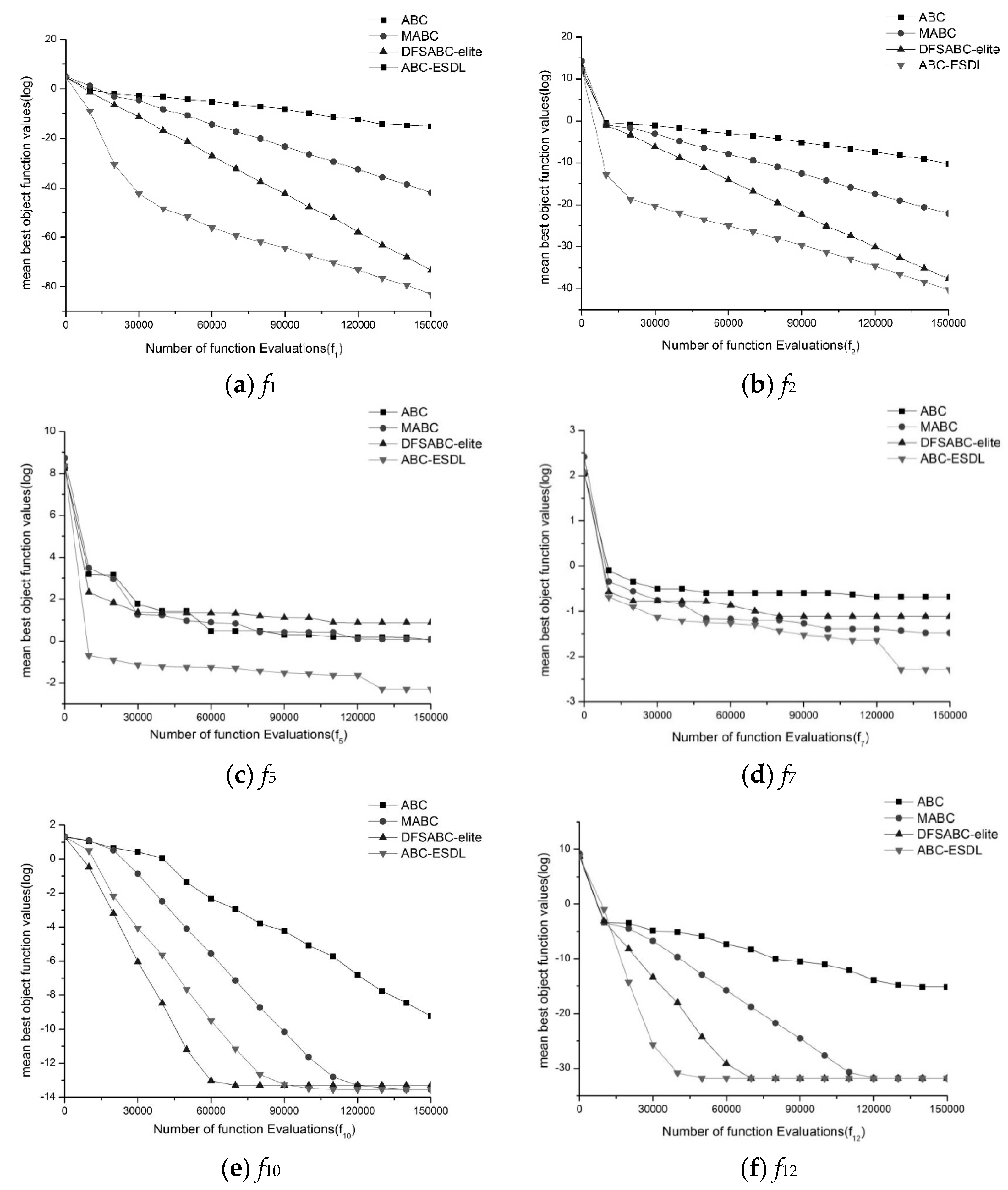
Figure 2 presents the convergence processes of ABC-ESDL, DFSABC-elite, MABC, and ABC on selected problems with D = 30. As seen, ABC-ESDL was faster than DFSABC-elite, MABC, and ABC. For f₁, f₂, f₁₀, and f₁₂, DFSABC-elite converged faster than MABC and ABC. For f₅, DFSABC-elite was the slowest algorithm. ABC was faster than DFSABC-elite on f₇. For f10, ABC-ESDL was slower than DFSABC-elite at the beginning search stage, and it was faster at the last search stage.

By the suggestions of [53,56], a nonparametric statistical test was used to compare the overall performances of seven ABCs. In the following, the mean rank of each algorithm on the whole benchmark set was calculated by the Friedman test.

Table 4. Mean ranks achieved by the Friedman test for D = 30 and 100.

Algorithms	Mean Rank
	D = 30	D = 100
ABC	6.50	6.67
GABC	4.58	5.33
IABC	4.08	4.42
MABC	3.79	3.58
ABCVSS	3.79	3.29
DFSABC-elite	3.29	2.67
ABC-ESDL	1.96	2.04

* The best rank for each dimension is shown in boldface.

gives the mean rank values of seven ABCs for D = 30 and 100. The smallest rank value meant that the corresponding algorithm obtained the best performance. For D = 30 and 100, ABC-ESDL achieved the best performances, and DFSABC-elite was in second place. For D = 30, both MABC and ABCVSS had the same rank. When the dimension increased to 100, ABCVSS obtained a better rank than MABC.

5.4. Effects of Different Strategies

There are two modifications in ABC-ESDL: elite strategy (ES) and dimension learning (DL). To investigate the effects of different strategies (ES and DL), we tested different combinations between ABC, ES, and DL on the benchmark set. The involved combinations are listed as below:

• ABC without ES or DL;
• ABC-ES: ABC with elite strategy;
• ABC-DL: ABC with dimension learning;
• ABC-ESDL: ABC with elite strategy and dimension learning.

For the above four ABC algorithms, the parameter settings were kept the same as in Section 5.3. The parameters MaxFEs, N, limit, and M were set to 5000*D, 100, 100, and 5, respectively. All algorithms ran 100 times for each problem for D = 30 and 100.

Table 5. Comparison of ABC with different strategies (D = 30).

Problems	ABC		ABC-ES		ABC-DL		ABC-ESDL
	Mean	Std Dev	Mean	Std Dev	Mean	Std Dev	Mean	Std Dev
f1	1.14 × 10−15	3.58 × 10−16	1.37 × 10−33	2.51 × 10−34	4.67 × 10−17	4.78 × 10−17	2.30 × 10−82	1.13 × 10−80
f2	1.49 × 10−10	2.34 × 10−10	2.82 × 10−21	3.23 × 10−21	1.02 × 10−10	3.46 × 10−11	3.13 × 10−41	6.81 × 10−40
f3	1.05 × 104	3.37 × 103	6.71 × 103	2.94 × 103	7.62 × 103	3.27 × 103	3.61 × 103	1.28 × 103
f4	4.07 × 101	1.72 × 101	2.21 × 100	2.06 × 100	3.82 × 101	1.24 × 101	2.11 × 10−1	7.20 × 10−1
f5	1.28 × 100	1.05 × 100	3.88 × 101	1.65 × 101	9.63 × 10−2	1.09 × 10−2	1.16 × 10−3	2.08 × 10−2
f6	0	0	0	0	0	0	0	0
f7	1.54 × 10−1	2.93 × 10−1	9.40 × 10−2	1.77 × 10 −2	2.82 × 10−1	2.51 × 10−2	1.46 × 10−2	2.64 × 10−2
f8	−12,490.5	5.87 × 10+1	−12557.8	1.62 × 101	−12,533.1	1.93 × 102	−12,569.5	4.65 × 10−11
f9	7.11 × 10−15	2.28 × 10−15	7.94 × 10−14	2.58 × 10−15	2.43 × 10−15	0	0	0
f10	1.60 × 10−9	4.32 × 10−9	3.49 × 10−14	1.87 × 10−14	6.45 × 10−10	1.99 × 10−14	2.82 × 10−14	2.00 × 10−14
f11	1.04 × 10−13	3.56 × 10−13	7.55 × 10−3	6.38 × 10−3	2.49 × 10−15	1.52 × 10−15	0	0
f12	5.46 × 10−16	3.46 × 10−16	1.57 × 10−32	0	1.56 × 10−19	0	1.57 × 10−32	5.81 × 10−47
w/t/l	11/1/0		10/2/0		11/1/0		-

* The best result for each function is shown in boldface.

presents the comparison of ABC-ESDL, ABC-ES, ABC-DL, and ABC for D = 30. The best result for each function is shown in boldface. From the results, all four algorithms obtained the same results on f₆. ABC was worse than ABC-ES on eight problems, but ABC-ES obtained worse results on three problems. ABC-DL outperformed ABC on ten problems, while ABC-DL was worse than ABC on only one problem. ABC-ESDL outperformed ABC-DL and ABC on 11 problems. Compared to ABC-ES, ABC-ESDL was better on ten problems, and both of them had the same performances on the rest of the two problems.

Table 6. Comparison of ABC with different strategies (D = 100).

Problems	ABC		ABC-ES		ABC-DL		ABC-ESDL
	Mean	Std Dev	Mean	Std Dev	Mean	Std Dev	Mean	Std Dev
f1	7.42 × 10−15	5.89 × 10−15	1.53 × 10−27	2.87 × 10−26	3.96 × 10−15	1.91 × 10−14	6.82 × 10−85	3.06 × 10−83
f2	1.09 × 10−9	4.56 × 10−9	1.11 × 10−16	1.18 × 10−15	9.41 × 10−10	1.86 × 10−9	1.02 × 10−52	1.76 × 10−51
f3	1.13 × 105	2.62 × 104	9.39 × 104	2.63 × 104	1.08 × 105	3.91 × 104	7.82 × 104	8.55 × 104
f4	8.91 × 101	4.37 × 101	3.44 × 101	3.44 × 101	8.73 × 101	7.92 × 100	2.66 × 101	1.32 × 101
f5	3.46 × 100	4.29 × 100	1.19 × 102	1.19 × 102	2.21 × 10−1	1.83 × 100	1.92 × 10−3	3.22 × 10−2
f6	1.58 × 100	1.68 × 100	0	0	3.13 × 100	6.59 × 100	0	0
f7	1.96 × 100	2.57 × 100	1.87 × 10−1	1.35 × 10−1	1.43 × 100	1.04 × 100	8.34 × 10−2	9.15 × 10−2
f8	−40,947.5	7.34 × 102	−41,762.1	5.95 × 102	−41,240.7	8.02 × 102	−41,898.3	1.63 × 10−10
f9	1.83 × 10−11	2.27 × 10−11	1.29 × 10−9	3.78 × 10−8	2.07 × 10−6	5.32 × 10−5	0	0
f10	3.54 × 10−9	7.28 × 10−10	1.57 × 10−13	4.35 × 10−14	2.17 × 10−9	5.06 × 10−9	1.25 × 10−13	5.61 × 10−14
f11	1.12 × 10−14	9.52 × 10−15	9.13 × 10−4	1.49 × 10−2	1.89 × 10−15	7.52 × 10−15	0	0
f12	4.96 × 10−15	3.29 × 10−15	4.29 × 10−28	8.78 × 10−27	3.21 × 10−18	2.19 × 10−17	4.71 × 10−33	7.50 × 10−48
w/t/l	12/0/0		11/1/0		12/0/0		-

* The best result for each function is shown in boldface.

gives the results of ABC-ESDL, ABC-ES, ABC-DL, and ABC for D = 100. The best result for each function is shown in boldface. Similar to D = 30, we can get the same conclusion. ABC-ESDL performed better than ABC, ABC-ES, and ABC-DL. ABC-ES was better than ABC-DL on most test problems, and both of them outperformed the original ABC.

For the above analysis, ABC with a single strategy (ES or DL) achieved better results than the original ABC. By introducing ES and DL into ABC, the performance of ABC-ESDL was further enhanced, and it outperformed ABC and ABC with a single strategy. This demonstrated that both ES and DL were helpful in strengthening the performance of ABC.

5.5. Results of the CEC 2013 Benchmark Set

In Section 5.3, ABC-ESDL was tested on several classical benchmark functions. To verify the performance of ABC-ESDL on difficult functions, the 2013 IEEE Congress on Evolutionary (CEC 2013) benchmark set was utilized in this section [60].

In the experiments, ABC-ESDL was compared with ABC, GABC, MABC, ABCVSS, and DFSABC-elite on the CEC benchmark set with D = 30. By the suggestions of [60], MaxFEs was set to 10,000*D. For other parameters, the same settings were used as described in Section 5.3. For each test function, each algorithm was run 51 times. Throughout the experiments, the mean function error value (f(X) − f(X*)) was reported, where X was the best solution found by the algorithm in a run, and X* was the global optimum of the test function [60].

Table 7. Results on the CEC 2013 benchmark set.

Problems	ABC		GABC		MABC		ABCVSS		DFSABC-elite		ABC-ESDL
	Mean	Std Dev	Mean	Std Dev	Mean	Std Dev	Mean	Std Dev	Mean	Std Dev	Mean	Std Dev
f1	6.82 × 10−14	2.18 × 10−13	5.71 × 10−13	9.44 × 10−14	4.55 × 10−14	1.33 × 10−12	6.82 × 10−14	1.88 × 10−12	4.55 × 10−14	1.19 × 10−12	7.29 × 10−5	1.66 × 10−3
f2	1.05 × 105	5.86 × 106	3.43 × 107	5.63 × 106	1.88 × 107	4.34 × 107	2.54 × 105	7.24 × 105	1.98 × 107	4.55 × 107	2.55 × 106	1.16 × 106
f3	2.49 × 109	6.24 × 109	1.05 × 1010	1.19 × 109	5.58 × 107	2.94 × 107	1.89 × 108	5.60 × 108	7.83 × 107	2.26 × 107	1.95 × 106	3.08 × 106
f4	6.81 × 103	2.09 × 103	3.51 × 105	1.48 × 104	9.83 × 103	2.56 × 103	8.18 × 103	2.05 × 103	6.58 × 103	1.79 × 103	5.94 × 103	1.81 × 105
f5	4.97 × 10−10	8.53 × 10−9	4.70 × 10−13	5.65 × 10−14	5.68 × 10−14	1.52 × 10−12	1.71 × 10−13	6.98 × 10−12	1.02 × 10−13	2.50 × 10−12	1.07 × 10−3	3.00 × 10−3
f6	1.73 × 100	5.07 × 100	1.77 × 102	1.82 × 100	1.76 × 100	6.81 × 100	2.25 × 100	7.12 × 100	1.67 × 100	1.14 × 100	8.58 × 10−1	3.57 × 10−1
f7	1.29 × 102	3.58 × 101	4.09 × 102	1.29 × 101	1.06 × 101	3.52 × 101	1.26 × 101	3.96 × 101	9.27 × 100	2.53 × 100	7.16 × 100	2.15 × 100
f8	2.10 × 100	5.96 × 100	2.13 × 101	3.51 × 10−2	2.09 × 100	5.97 × 100	2.11 × 100	5.97 × 100	2.10 × 100	5.96 × 100	2.08 × 100	5.95 × 100
f9	3.02 × 101	8.69 × 100	1.40 × 102	2.43 × 101	2.79 × 101	8.69 × 100	3.05 × 101	8.81 × 100	3.04 × 101	8.47 × 100	2.97 × 101	8.08 × 100
f10	3.40 × 10−1	8.22 × 10−1	1.43 × 100	8.48 × 10−1	1.62 × 10−1	4.60 × 10−1	3.05 × 10−1	1.32 × 10−1	2.46 × 10−1	5.59 × 10−1	2.51 × 10−2	6.91 × 10−2
f11	3.30 × 10−13	4.73 × 10−13	1.54 × 10−13	2.86 × 10−14	1.14 × 10−14	3.24 × 10−14	1.71 × 10−14	4.30 × 10−14	5.68 × 10−15	2.50 × 10−15	6.81 × 10−4	1.91 × 10−4
f12	3.14 × 101	8.42 × 101	1.60 × 103	5.64 × 101	1.57 × 101	5.52 × 100	2.46 × 101	6.01 × 101	2.20 × 101	5.61 × 100	1.51 × 101	4.91 × 100
f13	3.14 × 101	9.36 × 100	1.81 × 103	5.60 × 101	2.63 × 101	7.29 × 100	2.27 × 101	7.64 × 100	2.13 × 101	6.65 × 100	2.70 × 101	7.51 × 100
f14	1.09 × 100	4.05 × 100	2.85 × 100	1.28 × 100	2.48 × 10−1	5.23 × 10−1	6.25 × 10−3	1.14 × 10−2	2.10 × 10−2	1.80 × 10−2	7.47 × 10−1	3.05 × 10−1
f15	3.49 × 103	1.22 × 102	1.57 × 104	6.11 × 102	3.21 × 103	1.06 × 102	2.65 × 103	1.28 × 102	5.09 × 103	1.40 × 102	2.62 × 103	1.10 × 102
f16	1.65 × 100	5.11 × 100	2.07 × 100	2.57 × 10−1	1.57 × 100	3.98 × 100	2.15 × 100	5.66 × 100	2.49 × 100	5.97 × 100	8.49 × 10−1	3.75 × 10−1
f17	3.11 × 100	8.81 × 101	1.07 × 102	1.06 × 102	3.04 × 100	8.67 × 100	3.04 × 100	8.66 × 100	3.27 × 100	8.66 × 100	3.09 × 100	8.76 × 100
f18	3.88 × 102	1.01 × 102	1.76 × 103	5.02 × 102	1.90 × 102	6.59 × 101	3.45 × 102	9.27 × 101	2.84 × 102	7.53 × 101	1.44 × 102	4.99 × 101
f19	1.07 × 10−1	3.67 × 10−1	2.25 × 100	2.94 × 10−1	6.81 × 10−2	2.26 × 10−2	1.54 × 10−1	6.58 × 10−1	4.56 × 10−2	2.29 × 10−2	4.49 × 10−2	9.31 × 10−2
f20	1.54 × 101	4.17 × 100	5.00 × 101	6.93 × 100	1.46 × 101	4.11 × 100	1.48 × 101	4.11 × 100	1.46 × 101	4.02 × 100	1.41 × 101	3.82 × 100
f21	2.01 × 102	5.59 × 101	3.67 × 102	9.04 × 101	2.06 × 102	5.77 × 101	2.18 × 102	6.27 × 101	2.00 × 102	9.20 × 101	1.02 × 102	5.31 × 101
f22	1.16 × 102	3.71 × 101	7.47 × 101	2.64 × 101	1.05 × 102	3.06 × 101	1.15 × 102	4.13 × 101	1.19 × 102	3.20 × 101	1.47 × 101	2.04 × 100
f23	5.53 × 103	1.52 × 102	2.16 × 104	8.78 × 103	4.11 × 103	1.35 × 102	5.57 × 103	1.63 × 102	5.87 × 103	1.74 × 102	3.18 × 103	1.26 × 102
f24	3.02 × 102	8.33 × 101	6.00 × 102	7.56 × 101	2.88 × 102	8.13 × 101	2.86 × 102	8.27 × 101	2.86 × 102	8.09 × 101	2.80 × 102	8.07 × 101
f25	3.15 × 102	8.88 × 101	7.16 × 102	9.05 × 100	2.96 × 102	8.53 × 101	3.02 × 102	8.67 × 101	3.00 × 102	8.53 × 101	3.00 × 102	8.56 × 101
f26	2.01 × 102	5.73 × 101	2.07 × 102	3.95 × 10−1	2.01 × 102	5.72 × 101	2.01 × 102	5.73 × 101	2.01 × 102	5.72 × 101	2.00 × 102	5.71 × 101
f27	4.02 × 102	1.34 × 101	3.81 × 103	6.27 × 102	1.11 × 103	3.00 × 102	4.02 × 102	1.90 × 101	4.02 × 102	1.14 × 101	4.00 × 102	1.26 × 101
f28	1.64 × 102	7.10 × 101	4.27 × 103	5.67 × 102	3.00 × 102	8.54 × 101	3.13 × 102	9.29 × 101	3.00 × 102	8.70 × 101	1.04 × 102	8.45 × 101
w/t/l	25/0/3		25/0/3		20/0/8		21/0/7		22/1/5

* The best result for each function is shown in boldface.

presents the computational results of ABC-ESDL, DFSABC-elite, ABCVSS, MABC, GABC, and ABC on the 2013 IEEE Congress on Evolutionary (CEC 2013) benchmark set, where “Mean” indicates the mean function error values and “Std Dev” represents the standard deviation. The best result for each function is shown in boldface. From the results, ABC-ESDL outperformed ABC and GABC on 25 functions, but it was worse on the rest of the three functions. Compared to MABC, ABC-ESDL achieved better results on 20 functions, but MABC was better than ABC-ESDL on the rest of the eight functions. ABC-ESDL performed better than ABCVSS and DFSABC-elite on 21 and 22 functions, respectively. From the above analysis, even for difficult functions, ABC-ESDL still obtained better performances than the compared algorithms.

6. Conclusions

To balance exploration and exploitation, an improved version of ABC, called ABC-ESDL, is proposed in this paper. In ABC-ESDL, there are two modifications: elite strategy (ES) and dimension learning (DL). The elite strategy is used to guide the search. Good solutions are selected into the elite set. These elite solutions are used to modify the search model. To maintain the size of the elite set, a simple replacement method is employed. In dimension learning, the difference between different dimensions can achieve a large jump to help trapped solutions escape from local minima. The performance of our approach ABC-ESDL is verified on twelve classical benchmark functions (with dimensions 30 and 100) and the 2013 IEEE Congress on Evolutionary (CEC 2013) benchmark set.

Computational results of ABC-ESDL are compared with ABC, GABC, IABC, MABC, ABCVSS, and DFSABC-elite. For D = 30 and 100, ABC-ESDL is not worse than ABCVSS, MABC, IABC, GABC, and ABC. DFSABC-elite is better than ABC-ESDL on only one problem for D = 30 and two problems for D = 100. For the rest of problems, ABC-ESDL outperforms DFSABC-elite. For the 2013 IEEE Congress on Evolutionary (CEC 2013) benchmark set, ABC-ESDL still achieves better performances than the compared algorithms.

Another experiment investigates the effectiveness of ES and DL. Results show that ES or DL can achieve improvements. ABC with two strategies (both ES and DL) surpasses ABC and ABC with a single strategy (ES or DL). It confirms the effectiveness of our proposed strategies.

For the onlooker bees, offspring is generated for each elite solution in the elite set. So, an onlooker bee generates M new solutions when a parent solution X_i is selected. This complexity will increase the computational time. To reduce the effects of such computational effort, a small parameter M is used. In the future work, other strategies will be considered to replace the current method. In addition, more test functions [61] will be considered to further verify the performance of our approach.

References

- Kennedy, J. Particle Swarm Optimization. In Proceedings of the 1995 International Conference on Neural Networks, Perth, WA, Australia, 27 November–1 December 1995; Volume 4, pp. 1942–1948. [Google Scholar]
- Wang, F.; Zhang, H.; Li, K.S.; Lin, Z.Y.; Yang, J.; Shen, X.L. A hybrid particle swarm optimization algorithm using adaptive learning strategy. Inf. Sci. 2018, 436–437, 162–177. [Google Scholar] [CrossRef]
- Souza, T.A.; Vieira, V.J.D.; Souza, M.A.; Correia, S.E.N.; Costa, S.L.N.C.; Costa, W.C.A. Feature selection based on binary particle swarm optimisation and neural networks for pathological voice detection. Int. J. Bio-Inspir. Comput. 2018, 11, 91–101. [Google Scholar] [CrossRef]
- Sun, C.L.; Jin, Y.C.; Chen, R.; Ding, J.L.; Zeng, J.C. Surrogate-assisted cooperative swarm optimization of high-dimensional expensive problems. IEEE Trans. Evol. Comput. 2017, 21, 644–660. [Google Scholar] [CrossRef]
- Wang, H.; Wu, Z.J.; Rahnamayan, S.; Liu, Y.; Ventresca, M. Enhancing particle swarm optimization using generalized opposition-based learning. Inf. Sci. 2011, 181, 4699–4714. [Google Scholar]
- Karaboga, D. An Idea Based on Honey Bee Swarm for Numerical Optimization; Technical Report-tr06; Engineering Faculty, Computer Engineering Department, Erciyes University: Kayseri, Turkey, 2005. [Google Scholar]
- Amiri, E.; Dehkordi, M.N. Dynamic data clustering by combining improved discrete artificial bee colony algorithm with fuzzy logic. Int. J. Bio-Inspir. Comput. 2018, 12, 164–172. [Google Scholar] [CrossRef]
- Meang, Z.; Pan, J.S. HARD-DE: Hierarchical archive based mutation strategy with depth information of evolution for the enhancement of differential evolution on numerical optimization. IEEE Access 2019, 7, 12832–12854. [Google Scholar] [CrossRef]
- Meang, Z.; Pan, J.S.; Kong, L.P. Parameters with adaptive learning mechanism (PALM) for the enhancement of differential evolution. Knowl.-Based Syst. 2018, 141, 92–112. [Google Scholar] [CrossRef]
- Yang, X.S. Engineering Optimization: An Introduction with Metaheuristic Applications; John Wiley & Sons: Etobicoke, ON, Canada, 2010. [Google Scholar]
- Wang, H.; Wang, W.; Sun, H.; Rahnamayan, S. Firefly algorithm with random attraction. Int. J. Bio-Inspir. Comput. 2016, 8, 33–41. [Google Scholar] [CrossRef]
- Wang, H.; Wang, W.J.; Cui, Z.H.; Zhou, X.Y.; Zhao, J.; Li, Y. A new dynamic firefly algorithm for demand estimation of water resources. Inf. Sci. 2018, 438, 95–106. [Google Scholar] [CrossRef]
- Wang, H.; Wang, W.J.; Cui, L.Z.; Sun, H.; Zhao, J.; Wang, Y.; Xue, Y. A hybrid multi-objective firefly algorithm for big data optimization. Appl. Soft Comput. 2018, 69, 806–815. [Google Scholar] [CrossRef]
- Wang, G.G.; Deb, S.; Coelho, L.S. Earthworm optimisation algorithm: A bio-inspired metaheuristic algorithm for global optimisation problems. Int. J. Bio-Inspir. Comput. 2018, 12, 1–22. [Google Scholar] [CrossRef]
- Yang, X.S.; Deb, S. Cuckoo Search via Levy Flights. Mathematics 2010, 1, 210–214. [Google Scholar]
- Zhang, M.; Wang, H.; Cui, Z.; Chen, J. Hybrid multi-objective cuckoo search with dynamical local search. Memet. Comput. 2018, 10, 199–208. [Google Scholar] [CrossRef]
- Wang, G.G. Moth search algorithm: A bio-inspired metaheuristic algorithm for global optimization problems. Memet. Comput. 2016, 10, 1–14. [Google Scholar] [CrossRef]
- Cui, Z.; Wang, Y.; Cai, X. A pigeon-inspired optimization algorithm for many-objective optimization problems. Sci. China Inf. Sci. 2019, 62, 070212. [Google Scholar] [CrossRef]
- Yang, X.S. A new metaheuristic bat-inspired algorithm. Comput. Knowl. Technol. 2010, 284, 65–74. [Google Scholar]
- Wang, Y.; Wang, P.; Zhang, J.; Cui, Z.; Cai, X.; Zhang, W.; Chen, J. A novel bat algorithm with multiple strategies coupling for numerical optimization. Mathematics 2019, 7, 135. [Google Scholar] [CrossRef]
- Cai, X.J.; Gao, X.Z.; Xue, Y. Improved bat algorithm with optimal forage strategy and random disturbance strategy. Int. J. Bio-Inspir. Comput. 2016, 8, 205–214. [Google Scholar] [CrossRef]
- Cui, Z.H.; Xue, F.; Cai, X.J.; Gao, Y.; Wang, G.G.; Chen, J.J. Detection of malicious code variants based on deep learning. IEEE Trans. Ind. Inf. 2018, 14, 3187–3196. [Google Scholar] [CrossRef]
- Cai, X.; Wang, H.; Cui, Z.; Cai, J.; Xue, Y.; Wang, L. Bat algorithm with triangle-flipping strategy for numerical optimization. Int. J. Mach. Learn. Cybern. 2018, 9, 199–215. [Google Scholar] [CrossRef]
- Wang, G.G.; Guo, L.H.; Gandomi, A.H.; Hao, G.S.; Wang, H.Q. Chaotic krill herd algorithm. Inf. Sci. 2014, 274, 17–34. [Google Scholar] [CrossRef]
- Wang, G.G.; Gandomi, A.H.; Alavi, A.H. An effective krill herd algorithm with migration operator in biogeography-based optimization. Appl. Math. Model. 2014, 38, 2454–2462. [Google Scholar] [CrossRef]
- Wang, G.G.; Gandomi, A.H.; Alavi, A.H. Stud krill herd algorithm. Neurocomputing 2014, 128, 363–370. [Google Scholar] [CrossRef]
- Wang, G.G.; Guo, L.H.; Wang, H.Q.; Duan, H.; Luo, L.; Li, J. Incorporating mutation scheme into krill herd algorithm for global numerical optimization. Neural Comput. Appl. 2014, 24, 853–871. [Google Scholar] [CrossRef]
- Grimaccia, F.; Gruosso, G.; Mussetta, M.; Niccolai, A.; Zich, R.E. Design of tubular permanent magnet generators for vehicle energy harvesting by means of social network optimization. IEEE Trans. Ind. Electron. 2018, 65, 1884–1892. [Google Scholar] [CrossRef]
- Karaboga, D.; Akay, B. A survey: Algorithms simulating bee swarm intelligence. Artif. Intell. Rev. 2009, 31, 61–85. [Google Scholar] [CrossRef]
- Kumar, A.; Kumar, D.; Jarial, S.K. A review on artificial bee colony algorithms and their applications to data clustering. Cybern. Inf. Technol. 2017, 17, 3–28. [Google Scholar] [CrossRef]
- Zhu, G.; Kwong, S. Gbest-guided artificial bee colony algorithm for numerical function optimization. Appl. Math. Comput. 2010, 217, 3166–3173. [Google Scholar] [CrossRef]
- Wang, H.; Wu, Z.J.; Rahnamayan, S.; Sun, H.; Liu, Y.; Pan, J.S. Multi-strategy ensemble artificial bee colony algorithm. Inf. Sci. 2014, 279, 587–603. [Google Scholar] [CrossRef]
- Karaboga, D.; Akay, B. A comparative study of artificial bee colony algorithm. Appl. Math. Comput. 2009, 214, 108–132. [Google Scholar] [CrossRef]
- Karaboga, D.; Gorkemli, B. A quick artificial bee colony (qABC) algorithm and its performance on optimization problems. Appl. Soft Comput. 2014, 23, 227–238. [Google Scholar] [CrossRef]
- Gao, W.; Liu, S. A modified artificial bee colony algorithm. Comput. Oper. Res. 2012, 39, 687–697. [Google Scholar] [CrossRef]
- Cui, L.Z.; Li, G.H.; Lin, Q.Z.; Du, Z.H.; Gao, W.F.; Chen, J.Y.; Lu, N. A novel artificial bee colony algorithm with depth-first search framework and elite-guided search equation. Inf. Sci. 2016, 367–368, 1012–1044. [Google Scholar] [CrossRef]
- Li, G.H.; Cui, L.Z.; Fu, X.H.; Wen, Z.K.; Lu, N.; Lu, J. Artificial bee colony algorithm with gene recombination for numerical function optimization. Appl. Soft Comput. 2017, 52, 146–159. [Google Scholar] [CrossRef]
- Yao, X.; Chan, F.T.S.; Lin, Y.; Jin, H.; Gao, L.; Wang, X.; Zhou, J. An individual dependent multi-colony artificial bee colony algorithm. Inf. Sci. 2019. [Google Scholar] [CrossRef]
- Kumar, D.; Mishra, K.K. Co-variance guided artificial bee colony. Appl. Soft Comput. 2018, 70, 86–107. [Google Scholar] [CrossRef]
- Yang, J.; Jiang, Q.; Wang, L.; Liu, S.; Zhang, Y.; Li, W.; Wang, B. An adaptive encoding learning for artificial bee colony algorithms. J. Comput. Sci. 2019, 30, 11–27. [Google Scholar] [CrossRef]
- Chen, X.; Tianfield, H.; Li, K. Self-adaptive differential artificial bee colony algorithm for global optimization problems. Swarm Evol. Comput. 2019, 45, 70–91. [Google Scholar] [CrossRef]
- Zhang, X.; Zhang, X. A binary artificial bee colony algorithm for constructing spanning trees in vehicular ad hoc networks. Ad Hoc Netw. 2017, 58, 198–204. [Google Scholar] [CrossRef]
- Zorarpacı, E.; Özel, S.A. A hybrid approach of differential evolution and artificial bee colony for feature selection. Expert Syst. Appl. 2016, 62, 91–103. [Google Scholar] [CrossRef]
- Yuan, X.; Wang, P.; Yuan, Y.; Huang, Y.; Zhang, X. A new quantum inspired chaotic artificial bee colony algorithm for optimal power flow problem. Energy Convers. Manag. 2015, 100, 1–9. [Google Scholar] [CrossRef]
- Dokeroglu, T.; Sevinc, E.; Cosar, A. Artificial bee colony optimization for the quadratic assignment problem. Appl. Soft Comput. 2019, 76, 595–606. [Google Scholar] [CrossRef]
- Kishor, A.; Singh, P.K.; Prakash, J. NSABC: Non-dominated sorting based multi-objective artificial bee colony algorithm and its application in data clustering. Neurocomputing 2016, 216, 514–533. [Google Scholar] [CrossRef]
- Wang, P.; Xue, F.; Li, H.; Cui, Z.; Xie, L.; Chen, J. A multi-objective DV-Hop localization algorithm based on NSGA-II in internet of things. Mathematics 2019, 7, 184. [Google Scholar] [CrossRef]
- Pan, J.S.; Kong, L.P.; Sung, T.W.; Tsai, P.W.; Snasel, V. α-Fraction first strategy for hierarchical wireless sensor networks. J. Internet Technol. 2018, 19, 1717–1726. [Google Scholar]
- Xue, X.S.; Pan, J.S. A compact co-evolutionary algorithm for sensor ontology meta-matching. Knowl. Inf. Syst. 2018, 56, 335–353. [Google Scholar] [CrossRef]
- Hashim, H.A.; Ayinde, B.O.; Abido, M.A. Optimal placement of relay nodes in wireless sensor network using artificial bee colony algorithm. J. Netw. Comput. Appl. 2016, 64, 239–248. [Google Scholar] [CrossRef] [Green Version]
- Wang, H.; Wu, Z.J.; Zhou, X.Y.; Rahnamayan, S. Accelerating artificial bee colony algorithm by using an external archive. In Proceedings of the IEEE Congress on Evolutionary Computation, Cancun, Mexico, 20–23 June 2013; pp. 517–521. [Google Scholar]
- Li, B.; Sun, H.; Zhao, J.; Wang, H.; Wu, R.X. Artificial bee colony algorithm with different dimensional learning. Appl. Res. Comput. 2016, 33, 1028–1033. [Google Scholar]
- Wang, H.; Wang, W.; Zhou, X.; Sun, H.; Zhao, J.; Yu, X.; Cui, Z. Firefly algorithm with neighborhood attraction. Inf. Sci. 2017, 382, 374–387. [Google Scholar] [CrossRef]
- Wang, H.; Sun, H.; Li, C.H.; Rahnamayan, S.; Pan, J.S. Diversity enhanced particle swarm optimization with neighborhood search. Inf. Sci. 2013, 223, 119–135. [Google Scholar] [CrossRef]
- Wang, G.G.; Tan, Y. Improving metaheuristic algorithms with information feedback models. IEEE Trans. Cybern. 2019, 49, 542–555. [Google Scholar] [CrossRef]
- Wang, H.; Rahnamayan, S.; Sun, H.; Omran, M.G.H. Gaussian bare-bones differential evolution. IEEE Trans. Cybern. 2013, 43, 634–647. [Google Scholar] [CrossRef]
- Wang, H.; Cui, Z.H.; Sun, H.; Rahnamayan, S.; Yang, X.S. Randomly attracted firefly algorithm with neighborhood search and dynamic parameter adjustment mechanism. Soft Comput. 2017, 21, 5325–5339. [Google Scholar] [CrossRef]
- Sun, C.L.; Zeng, J.C.; Pan, J.S.; Xue, S.D.; Jin, Y.C. A new fitness estimation strategy for particle swarm optimization. Inf. Sci. 2013, 221, 355–370. [Google Scholar] [CrossRef]
- Kiran, M.S.; Hakli, H.; Guanduz, M.; Uguz, H. Artificial bee colony algorithm with variable search strategy for continuous optimization. Inf. Sci. 2015, 300, 140–157. [Google Scholar] [CrossRef]
- Liang, J.J.; Qu, B.Y.; Suganthan, P.N.; Hernández-Díaz, A.G. Problem Definitions and Evaluation Criteria for the CEC 2013 Special Session and Competition on Real-Parameter Optimization; Tech. Rep. 201212; Computational Intelligence Laboratory, Zhengzhou University, Zhengzhou China and Nanyang Technological University: Singapore, 2013. [Google Scholar]
- Serani, A.; Leotardi, C.; Iemma, U.; Campana, E.F.; Fasano, G.; Diez, M. Parameter selection in synchronous and asynchronous deterministic particle swarm optimization for ship hydrodynamics problems. Appl. Soft Comput. 2016, 49, 313–334. [Google Scholar] [CrossRef] [Green Version]
Figure 1.
The flowchart of the proposed artificial bee colony-elite strategy and dimension learning (ABC-ESDL) algorithm.
Figure 2.
The convergence curves of ABC-ESDL, DFSABC-elite, MABC, and ABC on selected functions. (a) Sphere; (b) Schwefel 2.22; (c) Rosenbrock; (d) Quartic; (e) Ackley; and (f) Penalized.