Modeling, Simulation, and Temperature Control of a Thermal Zone with Sliding Modes Strategy
by
 , and
, and
Frank Florez
1,*, 
Pedro Fernández de Córdoba
2 ,
,
José Luis Higón
3,
Gerard Olivar
4 and
and
John Taborda
5 1
Faculty of Engineering and Architecture, Universidad Nacional de Colombia, Campus la Nubia, 170003 Manizales, Colombia
2
Instituto Universitario de Matemática Pura y Aplicada, Universitat Politècnica de València, Camino de Vera s/n, 46022 Valencia, Spain
3
Department of Architectural Graphic Expression, Universitat Politècnica de València, Camino de Vera s/n, 46022 Valencia, Spain
4
Faculty of Exact and Natural Sciences, Universidad Nacional de Colombia, Campus la Nubia, 170003 Manizales, Colombia
5
Faculty of Engineering, Universidad del Magdalena, 470003 Santa Marta, Colombia
*
Author to whom correspondence should be addressed.
Mathematics 2019, 7(6), 503; https://doi.org/10.3390/math7060503
Submission received: 27 March 2019
/
Revised: 15 May 2019
/
Accepted: 29 May 2019
/
Published: 2 June 2019
(This article belongs to the Special Issue Mathematical Modeling and Simulation in Science and Engineering Education)
Abstract
:To reduce the energy consumption in buildings is necessary to analyze individual rooms and thermal zones, studying mathematical models and applying new control techniques. In this paper, the design, simulation and experimental evaluation of a sliding mode controller for regulating internal temperature in a thermal zone is presented. We propose an experiment with small physical dimensions, consisting of a closed wooden box with heat internal sources to stimulate temperature gradients through operating and shut down cycles.
1. Introduction
In recent decades, building modeling and energy consumption in thermal zones have become a growing field of study for engineers and researchers [1]. These studies have been impulsed by different countries thanks to international agreements such as the Kyoto Protocol and the implementation of the sustainable development goals of the United Nations (UN). It has been realized that the high energetic consumption of HVAC systems in buildings, which in developed countries can account for 40% of the annual energy production, is a key factor in climatic change [2].
To minimize consumption in buildings, it is necessary to understand the main factors of energy waste, such as thermal comfort and human habits. Different tools have been developed to simulate thermodynamic processes in buildings [3,4]. For example, commercial programs such as TRNSYS and ENERGY PLUS allow representing an entire building and analyzing the effects of specific actions. Another important tool is mathematical modeling, which permits deeper numerical analysis and contributes to the development of new strategies and controllers for temperature regulation. At the same time, this allows reducing energy consumption [5].
The representation of a entire building consisting of different levels and a large number of rooms in each level, is a complex task especially if geometrical and physical characteristics, environmental conditions and relations with external bodies are taken into account. To simplify the problem, only individual and closed rooms are analyzed, and in subsequent stages the results are extrapolated to the entire building. The analysis of a single room as a thermal zone is reduced to capturing the thermodynamic processes in the room. This includes evaluating the different heat sources, both external and internal. Examples of external heat sources include sun radiation and surrounding bodies at different temperatures. Possible internal heat sources include electronic equipment and occupants. Some factors and phenomenona are easily handled, while others require important mathematical modeling in order to be captured. In order to meet these requirements without increasing the complexity of the mathematical model one makes simplifications that maintain the predominant dynamics of the problem [6].
There are many choices of a mathematical model, depending on factors such as accuracy, computational cost and adaptability. In many cases, high accuracy needs powerful electronic equipment for sensing and processing. If implemented, this often drives costs beyond the budget. Additionally, the more specific a mathematical model is, the more difficult its electronic implementation will be, including modifications and variations in a case study. Another important factor is the tuning of parameters in the model. Tuning strategies based on large databases or combinations of modeling strategies in order to obtain the maximum amount of information about the study case are found in [7,8,9].
Some modeling options are mentioned below: Ref. [5] presents a method for modeling room temperature based on the laws of thermodynamics resulting in an Armax model for control purposes. Ref. [10] uses the Zokolov mathematical model, which is based on heat balance with quasi-steady-state approximations to determine the average internal temperature. For more detailed models, it is possible to include different thermal phenomena such as infiltration and thermal inertia, as in [11], where the mass and energy conservation principle was used. However, in the majority of research it is acceptable to use reduced order models. The Lumped Parameter Methods (LPM) allow a choice among a large variety of structures and orders. Refs. [6,12] use circuits of 4th and 7th order to model single thermal zones, while Refs. [13,14] use simplifications and apply different control techniques.
An aspect as important as the mathematical model itself is the control strategy. This is so because some of the thermal zones inputs are constantly changing. Thus it becomes necessary to rely on a central controller that regulates the internal variables to achieve the objectives of thermal comfort and energy savings. Strategies such as the model predictive control (MPC) are accepted within the scientific community as a good alternative in thermal applications [15,16,17,18]. This technique has been compared with classic controllers such as PID [19] and been shown to perform better. Refs. [20,21] propose cooperative work with fuzzy controllers that exhibits an energy savings of about , demonstrating that the study of other techniques cannot be disregarded.
However, the study of alternative control techniques is not a easy task, especially in experimental investigations. To minimize problems in the evaluation of new control strategies, some researchers have been using reduced scale models. The latter allow the creation of sensed thermal zones with minimal resources and minimize the effect of environmental conditions. This effect is typically one of the most common factors in the failure of new control strategies [22,23,24,25].
In this article, we show how to use the Sliding Control strategy for regulation of the temperature in a thermal zone. This technique is normally used for commuted systems as power converters, but it is robust enough to be implemented in different applications [26,27,28,29,30]. For the evaluation of the control technique, an experiment with a scale reduced model was planned. The experiment consisted of a wooden box equipped with an internal lamp to simulate a heater in a room, in a cold climate environment. In the first stages of the experiment, a mathematical modeling technique was built and tuned with an experimental database. This allowed the development of a simulator that reproduced the experimental results with high accuracy. Subsequently we programmed an electronic card to drive the internal lamp according to the control rule.
This article is organized as follows: Section 2 presents the mathematical models used to represent the proposed experiment. Section 3 describes in detail the elements and places used in the tests. In Section 4 the process for tuning parameters is shown and the experimental and simulation results are compared. Finally, in Section 5, we present the control technique and the mathematical description necessary to simulate and complete the experimental test. Section 6 presents conclusions and suggests future work.
2. Mathematical Model
The lumped parameter technique is a methodology for modeling buildings, based on an analogy between thermal and electrical phenomena. Temperature is represented by voltage, heat flux by electric current, and thermal resistance is defined as the resistance to heat transfer through walls, and represented by an electrical resistance [31]. The resulting circuit must include a series of resistances associated with the different heat transfer processes, and capacitors that represent the wall’s capacity to accumulate energy. In the literature it is possible to find different configurations and circuits, which allows choosing different models to solve the problem according to information quantity, physical characteristics, internal gains and others factors [32].
In the Lumped Parameter Models the heat flux is assumed in one direction, the orientation is defined by the difference between the environmental and internal temperature. In case of a higher external temperature, the sequence followed for the thermal energy is as follows: first, transfer from the external air to the exterior surface of each wall; next, conduction through the walls; finally, transfer from the interior surface wall to the interior air in the zone. The reverse process takes place when the internal temperature is higher than the environmental temperature.
2.1. Full Scale Model
Figure 1 shows a RC circuit equivalent to one closed room with four walls, a roof and a floor. This configuration of the LPM is called Full Scale Model [6,7,8,9,10,11,12,13,14,15,16,17,18,19,20,21,22,23,24,25,26,27,28,29,30,31,32,33]. It is characterized by including branches for the different surfaces, each branch incorporating resistances for the convection, radiation and conduction processes. The nomenclature uses two subscripts i and j; the first one indicates the surface , and the second one indicates the position . The subscript “in” corresponds to the interior elements, “mid” to conduction resistances, and “ex” represents the exterior elements. Thus, e.g., the resistance corresponds to the heat transfer process between the interior face and the interior air.
The conduction resistance for the corresponding wall is calculated according to Equation (1), the interior and exterior resistances are calculated with Equation (2). Here denotes the emissivity coefficient of the material, and h denotes the convection coefficient which must be tuned experimentally. The thermal capacity of each wall and the air contained in the zone is defined by Equation (3):
The whole model contains 31 fixed parameters: capacitors, resistances, one single time variant input (the environmental temperature ), and finally 13 state variables associated with the internal and external surface temperatures together with the internal air temperature. All temperatures are calculated as the voltage over the capacitors, connecting the temperature with the capacitor , and the internal air temperature T with the capacitor . Applying circuit theory it is possible to determine one set of differential equations to calculate the temperature evolution:
Above, represents the power of the internal gains and u their state (active or inactive).
2.2. Simplified Model
Another useful structure is presented in Figure 2; this circuit provides a simplified model and, in many cases, is enough to analyze a thermal zone with minimal parameters. This model requires 18 fixed parameters, one single input and only two state variables, corresponding to the wall temperature and the internal temperature ( and T respectively). In this case, the conduction resistance is denoted with only one subscript i, and the internal and external resistances carry one additional subscript j to indicate their positions. Important elements are the calculation of and ; in this structure, the resistance is calculated with one half of the wall’s thickness, and the capacitor uses the entire superfice area. The order reduction in this model is given by disregarding the radiation process that, in transitional states, hardly contributes to the general dynamics. Thus, the internal and external resistances are calculated with the convection coefficient.
In order to calculate the set of differential equations, the circuit must be simplified by reducing the resistors; the external face is calculated by the parallel resistor as , where is the linear addition of the conduction and convection resistors . Similarly, the internal face resistor is calculated using the corresponding convection coefficient for the resistor . The final results are shown in Equations (7) and (8):
3. Experimental Setup
Using the concept of reduced scale models for the evaluation of the controller, a closed container was built with a chipboard working as a thermal zone. Such elements are regularly used in kitchen furniture. The dimensions of the container are 70 cm × 40 cm × 58 cm with 15.8 mm of wall thickness; additionally, it is lifted 10 cm from the ground with plastic legs that limit heat transmission by contact with the ground. In Table 1 additional data associated with the materials used in the experiment are presented.
The box was equipped with: one 60 W incandescent internal lamp with infrared light to simulate a heater in a closed room; one temperature and humidity sensor (Data Logger Whler CDL 210) inside the box, and another one outside the box for registering environmental conditions.
Figure 3 shows the wooden box with the lamp and temperature sensor ready to start the experiment. All the tests were carried out in closed spaces (in order to minimize the effect of environmental changes) at Polytechnic University of Valencia (Spain). The first two data recompilations were done in open loop, with the objective of generating enough information to adjust the models and calculate the control parameters [34].
4. Adjusting the Models
For the dynamical analysis of the thermal zone built, it was necessary to develop a simulator to reproduce the experimental results. The mathematical model described in Section 2.1 needs to be adjusted to the situation of the system. That is, the convection and radiation coefficients for internal and external faces had to be determined as functions of the state of the lamp. The activation state is called “charge” and the deactivation stage is called “discharge” in the rest of this work. The tuning is based on the experimental records obtained in open loop. Our strategy uses the registered data of the internal temperature and an optimization algorithm to minimize the error between simulation and experimental results.
The first test was done on 15 March 2018 and lasted 24 h (only the first 6 h were on charge). With the data compiled, the Pattern Search algorithm from the OptimTool of MATLAB was used. This tool requires a mathematical model, one objective function, and a set of output parameters. In this case, the mathematical model used is presented in Section 2.1. The objective function is shown in Equation (9). Finally, the set of output parameters defined are the internal convection coefficient , the external convection , the internal emissivity and the external emissivity .
As mentioned previously, the charge and discharge phases were analyzed individually, with the resulting coefficients presented in Table 2. With these parameters, the simulator was compared with the experimental results. This produced the results shown in Figure 4. The model’s accuracy with the adjusted parameters was tested by calculating the relative error shown in Equation (10). This led to an approximate error of 2.7%.
The second test in open loop was done on 13 April 2018 and lasted 11 days (10 days were on charge phase). The comparison between experimental and simulation is shown in Figure 5. In this case the relative error was about . This figure was plotted using a total amount of 4756 data. Among these, only in six cases does the difference between experimental and theoretical values exceed 2 degrees. It exceeds 1.5 degrees in 97 cases, while exceeding 1 degree in 461 cases. In all remaining 4295 cases the error lies below 1 degree.
5. Control Application
For the evaluation of the Sliding Control (SC) on the thermal zone, it was decided to use the second order model (presented in Section 2.2) because this scheme is easier to adapt to the control structure. In Figure 6, a reduction of the second order circuit is presented, with the internal gain driven by the SC to handle the internal temperature in the thermal zone.
The state variables defined by the controller are the temperature error and the heat flux shown in Equations (11) and (12). Here the desired temperature for the closed room is called reference temperature , and the switch u represents the internal gain state. With these variables and differentiating with respect to time, the state-space model can then be implemented by Equations (13) and (14):
To simplify the mathematical equations, the following parameters are defined:
The state variables are defined as functions of the constants previously defined (the ambient temperature, reference temperature, and the internal power source):
The SC determines the switch position with a trajectory function s based on the state variables,
Above, J and x are the vectors , and , , and is the parameter to be adjusted by the controller designer. The objective of this constant is to divide the space state in two sectors by a line with slope . This line is generated by the state variables that satisfy . In each zone, one system equilibrium () must be located, corresponding to the switch position (active/inactive).
The first case analyzed is the internal active source, with equilibrium coordinates presented in Equations (21) and (22). In this point the trajectory function is fulfilling the condition .
For the second case, the internal source is deactivated. The equilibrium conditions are shown in Equations (23) and (24). This point satisfies the condition :
Once the equilibrium analysis is done, the control laws can be established. Equation (25) shows the actions in the searching period. Equation (26) defines the control laws when the system is approaching the stability () tracking the sliding line. Here is a positive small constant arbitrarily determined.
To determine the slope of the sliding line () the evolution of the trajectory function must be evaluated with respect to time. Equation (28) shows that only the sliding parameter affects the incoming heat flux. Enforcing , the critical value can be determined as presented in Equation (29):
Based on the previous analysis, the slope of the sliding line was . With this constant and the system parameters defined, it was possible to develop the simulation of the thermal zone under the sliding control technique.
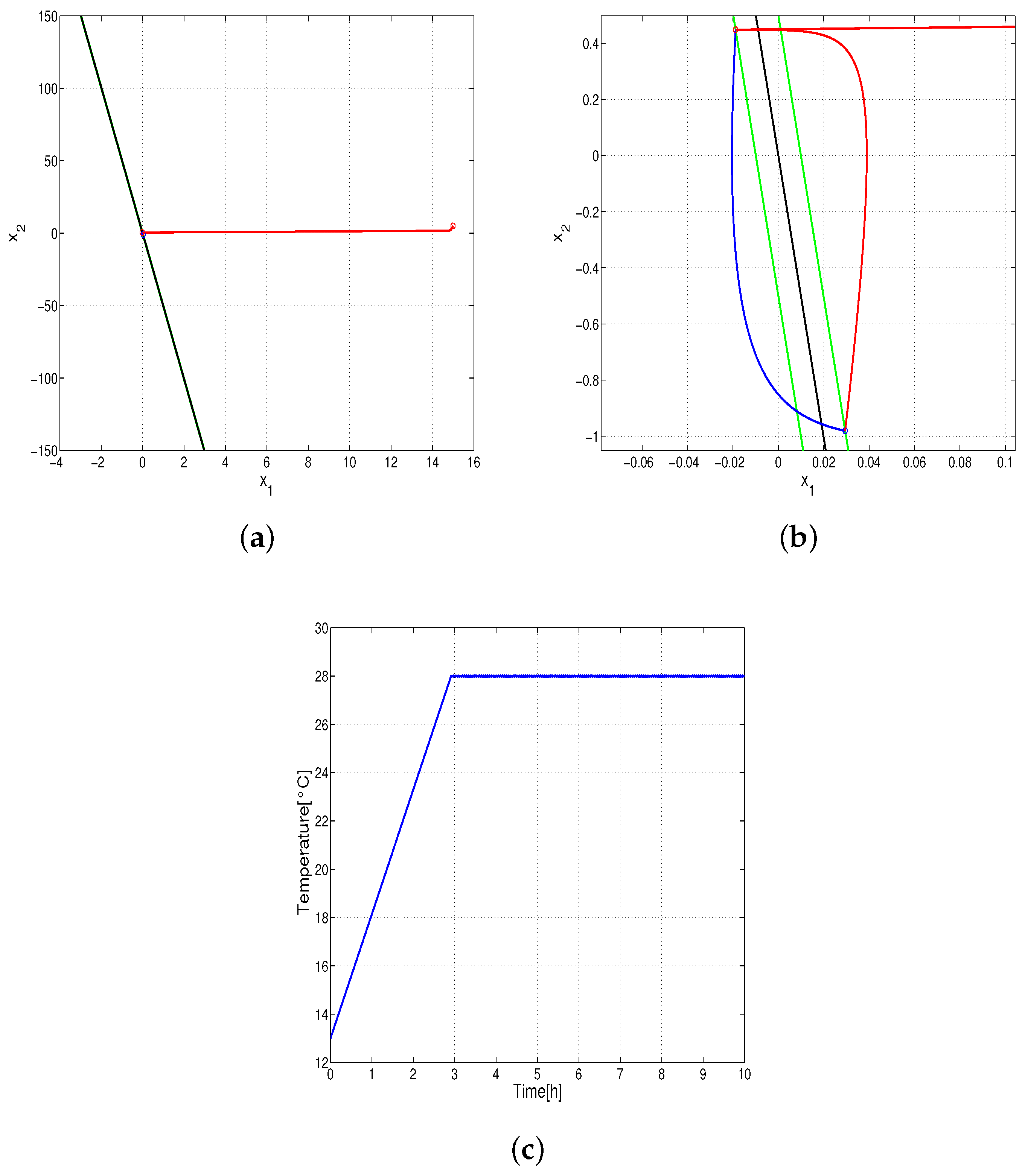
The simulation was designed with an ambient temperature of 16 C, a reference temperature of 28 C, and the hysteresis band with a fixed constant of . The results are presented in Figure 7. Here the black line represents the sliding surface, the green lines limits the hysteresis band, and the red and blue lines in Figure 7a correspond to the evolution of the state variables and as a function of the switch position; blue is for the active and red for the inactive . This first figure shows the search stage. Figure 7b shows the tracking stage and the oscillation of the system around the stability point (). Finally, Figure 7c presents the internal temperature that achieves the reference temperature and maintains its value satisfying the criteria.
We performed different experimental tests by programming the electronic card ESP32 LOLIN lite and measuring internal and external temperatures using a sensor DS18b20 with a sampling rate of 3 min. Figure 8 presents the results obtained after 65 h of experimentation. The first two pictures present the and variable evolution (searching and tracking stages). Figure 8c shows that the internal temperature achieves the reference temperature of 28 C. As in the case of the simulated results, this reference temperature (output variable) is achieved and it maintained the criterion.
6. Conclusions
An appropriate mathematical model can capture the thermodynamical behavior of a closed room, allowing analyzing its characteristics and determining the most important factors in energy consumption. In the energetic analysis of buildings, it is important to rely on algorithms and methods to estimate the heat transfer parameters that contribute to thermal leaks. In this work we proposed an experiment based on a piece of kitchen furniture with one internal lamp. Using the lumped parameter technique for modeling, it was possible to build a simulator to reproduce the internal temperature in the thermal zone.
In order to adjust the main parameters for the simulator, different tuning strategies were used. The best results were obtained by the algorithm called Pattern Search, in MATLAB. With this tool, and using the experimental data, we determine the transfer coefficients between the walls and the surrounding air. The full scale model to reproduce the experimental results with a relative error of less than .
To summarize, in this paper we tested the ability of the sliding control technique to regulate temperature in a thermal zone. The goals were achieved through the implementation of reduced scale models, through a set of important tools to experimentally verify the theories, and through new techniques of simulation and control in buildings. It is even possible to avoid many error sources in the mathematical models, such as environmental conditions and random disturbances. Furthermore, the test can be done with a low budget and without interrupting regular conditions in a real building.
The simulation and experimental results show that the technique control can be used to regulate the internal temperature of a thermal zone in regions with a low ambient temperature. This procedure can be extrapolated to different and bigger zones.
Future work to be done would be the introduction of disturbances test and the random opening of doors or windows. This could help to test the robustness of the controller. Furthermore, the evaluation of the energetic consumption in closed loop is necessary to define the savings in comparison with other control strategies.
Author Contributions
Conceptualization and methodology design: P.F.d.C. and J.L.H.; experiment development and data collection: F.F., J.L.H. and G.O.; data analysis and simulations: P.F.d.C., F.F. and J.T.; writing—original draft preparation: G.O. and F.F.; validation and writing—review and editing: P.F.d.C. and J.T.; funding acquisition: G.O., P.F.d.C. and J.L.H.
Funding
This investigation was supported by national doctoral program of the Colombian Administrative Department of Science Technology and Innovation (Colciencias), and the agreement “Analysis of the properties, applications and market opportunities of G-cover Coatings” closed between the Universitat Politècnica de València (Spain) and the Mexican company G-cover.
Acknowledgments
The authors thank to the Journal editors and the reviewers for their worthful suggestions and comments.
Conflicts of Interest
The authors declare no conflict of interest.
Nomeclature
| Sliding constant | |
| Stefan-Boltzman contant | |
| Material density | |
| Radiation coefficient | |
| Hysteresis band amplitude | |
| Thickness of the walls | |
| Material’s conductivity | |
| Surface area | |
| Convection coefficient | |
| s | Sliding trajectory |
| J | Sliding constants vector |
| x | State variables vector |
| Thermal resistance | |
| Surface thermal capacity | |
| Air thermal capacity | |
| Envelope thermal capacity | |
| Specific heat | |
| Surface temperature | |
| T | Zone temperature |
| Ambient temperature | |
| Superficial temperature | |
| Reference temperature | |
| Incoming heat flux | |
| u | Lamp state |
| Internal gain power | |
| Objective function | |
| Temperature error | |
| norm of function f: |
References
- Forgiarini, R.; Giraldo, N.; Lamberts, R. A review of human thermal comfort in the built environment. Energy Build. 2015, 105, 178–205. [Google Scholar] [CrossRef]
- Delgarm, N.; Sajadi, B.; Delgarm, S. Multi-objective optimization of building energy performance and indoor thermal comfort: A new method using artificial bee colony (ABC). Energy Build. 2016, 131, 42–53. [Google Scholar] [CrossRef]
- Underwood, C.; Yik, F. Modelling Methods for Energy in Buildings; Blackwell Science: Oxford, UK, 2004. [Google Scholar] [CrossRef]
- Park, H. Dynamic Thermal Modeling of Electrical Appliances for Energy Management of Low Energy Buildings. Ph.D. Thesis, University of Cergy-Pontoise, Cergy-Pontoise, France, 2014. [Google Scholar]
- Gorni, D.; Castilla, M.; Visioli, A. An efficient modelling for temperature control of residential buildings. Build. Environ. 2016, 103, 86–98. [Google Scholar] [CrossRef]
- Fazenda, P.; Lima, P.; Carreira, P. Context-based thermodynamic modeling of buildings spaces. Energy Build. 2016, 124, 164–177. [Google Scholar] [CrossRef]
- Bacher, P.; Madsen, H. Identifying suitable models for the heat dynamics of buildings. Energy Build. 2011, 43, 1511–1522. [Google Scholar] [CrossRef] [Green Version]
- Mba, L.; Meukam, P.; Kémajou, A. Application of Artificial Neural Network for Predicting the Indoor Air Temperature in Modern Building in Humid Region. Energy Build. 2016, 121, 32–42. [Google Scholar] [CrossRef]
- Lin, Y.; Middelkoop, T.; Barooah, P. Issues in identification of control-oriented thermal models of zones in multi-zone buildings. In Proceedings of the IEEE Conference on Decision and Control, Maui, HI, USA, 10–13 December 2012; pp. 6932–6937. [Google Scholar] [CrossRef]
- Anisimova, E.Y. Building Thermal Regime Modeling. Procedia Eng. 2017, 206, 795–799. [Google Scholar] [CrossRef]
- Ryzhov, A.; Ouerdane, H.; Gryazina, E.; Bischi, A.; Turitsyn, K. Model predictive control of indoor microclimate: Existing building stock comfort improvement. Energy Convers. Manag. 2019, 179, 219–228. [Google Scholar] [CrossRef]
- Bagheri, A.; Feldheim, V.; Thomas, D.; Ioakimidis, C. Energy Efficiency from to The walls The adjacent effects in simplified thermal model of buildings. In Proceedings of the ScienceDirect CISBAT 2017 International Conference, Lausanne, Switzerland, 6–8 September 2017. [Google Scholar]
- Luzi, M.; Vaccarini, M.; Lemma, M. A tuning methodology of Model Predictive Control design for energy efficient building thermal control. J. Build. Eng. 2019, 21, 28–36. [Google Scholar] [CrossRef]
- Fiorentini, M.; Wall, J.; Ma, Z.; Braslavsky, J.H.; Cooper, P. Hybrid model predictive control of a residential HVAC system with on-site thermal energy generation and storage. Appl. Energy 2017, 187, 465–479. [Google Scholar] [CrossRef] [Green Version]
- Massa Gray, F.; Schmidt, M. Thermal building modelling using Gaussian processes. Energy Build. 2016, 119, 119–128. [Google Scholar] [CrossRef]
- Ascione, F.; Bianco, N.; De Stasio, C.; Mauro, G.M.; Vanoli, G.P. Simulation-based model predictive control by the multi-objective optimization of building energy performance and thermal comfort. Energy Build. 2015, 111, 131–144. [Google Scholar] [CrossRef]
- Acosta, A.; González, A.I.; Zamarreño, J.M.; Álvarez, V. Energy savings and guaranteed thermal comfort in hotel rooms through nonlinear model predictive controllers. Energy Build. 2016, 129, 59–68. [Google Scholar] [CrossRef]
- Afram, A.; Janabi-shari, F. Theory and applications of HVAC control systems—A review of model predictive control (MPC). Build. Environ. 2014, 72, 343–355. [Google Scholar] [CrossRef]
- Nagarathinam, S.; Doddi, H.; Vasan, A.; Sarangan, V.; Venkata Ramakrishna, P.; Sivasubramaniam, A. Energy efficient thermal comfort in open-plan office buildings. Energy Build. 2017, 139, 476–486. [Google Scholar] [CrossRef]
- Smarra, F.; Jain, A.; de Rubeis, T.; Ambrosini, D.; D’Innocenzo, A.; Mangharam, R. Data-driven model predictive control using random forests for building energy optimization and climate control. Appl. Energy 2018, 226, 1252–1272. [Google Scholar] [CrossRef] [Green Version]
- Killian, M.; Mayer, B.; Kozek, M. Cooperative fuzzy model predictive control for heating and cooling of buildings. Energy Build. 2016, 112, 130–140. [Google Scholar] [CrossRef]
- Brastein, O.M.; Perera, D.W.; Pfeifer, C.; Skeie, N.O. Parameter estimation for grey-box models of building thermal behaviour. Energy Build. 2018, 169, 58–68. [Google Scholar] [CrossRef] [Green Version]
- Lirola, J.M.; Castañeda, E.; Lauret, B.; Khayet, M. A review on experimental research using scale models for buildings: Application and methodologies. Energy Build. 2017, 142, 72–110. [Google Scholar] [CrossRef] [Green Version]
- Coutinho, C.P.; Baptista, A.J.; Dias Rodrigues, J. Reduced scale models based on similitude theory: A review up to 2015. Eng. Struct. 2016, 119, 81–94. [Google Scholar] [CrossRef]
- Chew, L.W.; Glicksman, L.R.; Norford, L.K. Buoyant flows in street canyons: Comparison of RANS and LES at reduced and full scales. Build. Environ. 2018, 146, 77–87. [Google Scholar] [CrossRef]
- Chen, S.Y.; Gong, S.S. Speed tracking control of pneumatic motor servo systems using observation-based adaptative dynamic sliding-mode control. Mech. Syst. Signal Process. 2017, 94, 111–128. [Google Scholar] [CrossRef]
- Huang, Y.; Khajepour, A.; Ding, H.; Bagheri, F.; Bahrami, M. An energy-saving set-point optimizer with a sliding mode controller for automotive air-conditioning/refrigeration systems. Appl. Energy 2017, 188, 576–585. [Google Scholar] [CrossRef]
- Mironova, A.; Mercorelli, P.; Zedler, A.; Mironova, A.; Mercorelli, P. Robust Control using Sliding Mode Approach for Ice-Clamping Device activated by Thermoelectric Coolers. Int. Fed. Autom. Control 2016, 25, 470–475. [Google Scholar] [CrossRef]
- Norton, M.; Khoo, S.; Kouzani, A.; Stojcevski, A. Adaptive fuzzy multi-surface sliding control of multiple-input and multiple-output autonomous flight systems. IET Control Theory Appl. 2015, 9, 587–597. [Google Scholar] [CrossRef]
- He, T.; Li, L.; Zhu, J.; Zheng, L. A Novel Model Predictive Sliding Mode Control for AC/DC Converters with Output Voltage and Load Resistance Variations. In Proceedings of the 2016 IEEE Energy Conversion Congress and Exposition (ECCE), Milwaukee, WI, USA, 18–22 September 2016; pp. 1–6. [Google Scholar]
- Cengel, Y. Transferencia de Calor y Masa; McGraw Hill: Mexico City, Mexico, 2007. [Google Scholar]
- Fux, S.F.; Ashouri, A.; Benz, M.J.; Guzzella, L. EKF based self-adaptive thermal model for a passive house. Energy Build. 2014, 68, 811–817. [Google Scholar] [CrossRef]
- Lin, Y.; Middelkoop, T.; Barooah, P. Identification of control-oriented thermal models of rooms in multi-room buildings. In Proceedings of the 2012 IEEE 51st Annual Conference on Decision and Control (CDC), Maui, HI, USA, 10–13 December 2012. [Google Scholar]
- Florez, F.; Higón, J.; Conejero, J.A.; Córdoba, P.F.D. Modeling and Experimental verification of thermal properties of Thermo Sköld coating solutions. In Proceedings of the International Congress on Industrial and Applied Mathematics, Valencia, Spain, 15–19 July 2019; Volume 9. [Google Scholar]
Figure 1.
Circuit for a thermal zone using the full scale model.

Figure 2.
Circuit for a thermal zone using the simplified model.

Figure 3.
Wooden box used as scale reduced model.

Figure 4.
Simulated and experimental results in the first test.

Figure 5.
Simulated and experimental results in the second test.

Figure 6.
Reduced circuit of the simplified model with sliding modes control structure.

Figure 7.
Simulation results. (a) Theoretical development of the search stage. (b) Theoretical development of the tracking stage. (c) Theoretical internal temperature with the sliding mode control.
Figure 7.
Simulation results. (a) Theoretical development of the search stage. (b) Theoretical development of the tracking stage. (c) Theoretical internal temperature with the sliding mode control.

Figure 8.
Experimental results. (a) Experimental development of the search stage. (b) Experimental development of the tracking stage. (c) Experimental internal temperature with the sliding mode control.
Figure 8.
Experimental results. (a) Experimental development of the search stage. (b) Experimental development of the tracking stage. (c) Experimental internal temperature with the sliding mode control.


Table 1.
Parameters of the materials used in the experiment.
| Material | Parameter | Value |
|---|---|---|
| Wood | Conductivity | |
| Densitiy | ||
| Specific heat | ||
| Air | Density | |
| Specific heat |
Table 2.
Convection and radiation coefficients.
| Phase/Parameter | ||||
|---|---|---|---|---|
| Charge | 44.6875 | 11.1250 | 0.9430 | 0.9 |
| Discharge | 0 | 9.7324 | 0.0211 | 0.8805 |
© 2019 by the authors. Licensee MDPI, Basel, Switzerland. This article is an open access article distributed under the terms and conditions of the Creative Commons Attribution (CC BY) license (http://creativecommons.org/licenses/by/4.0/).
Share and Cite
MDPI and ACS Style
Florez, F.; Fernández de Córdoba, P.; Higón, J.L.; Olivar, G.; Taborda, J. Modeling, Simulation, and Temperature Control of a Thermal Zone with Sliding Modes Strategy. Mathematics 2019, 7, 503. https://doi.org/10.3390/math7060503
AMA Style
Florez F, Fernández de Córdoba P, Higón JL, Olivar G, Taborda J. Modeling, Simulation, and Temperature Control of a Thermal Zone with Sliding Modes Strategy. Mathematics. 2019; 7(6):503. https://doi.org/10.3390/math7060503
Chicago/Turabian StyleFlorez, Frank, Pedro Fernández de Córdoba, José Luis Higón, Gerard Olivar, and John Taborda. 2019. "Modeling, Simulation, and Temperature Control of a Thermal Zone with Sliding Modes Strategy" Mathematics 7, no. 6: 503. https://doi.org/10.3390/math7060503
Note that from the first issue of 2016, this journal uses article numbers instead of page numbers. See further details here.