Pricing to the Scenario: Price-Setting Newsvendor Models for Innovative Products

Abstract

In this paper, we consider a manufacturer who produces and sells a kind of innovative product in the monopoly market environment. Because the life cycle of an innovative product is usually shorter than its procurement lead time, one unique demand quantity (scenario) will occur in the selling season; thus, there is only one chance for the manufacturer to determine both optimal production quantity and optimal sale price. Considering this one-time feature of such a decision problem, a price-setting newsvendor model for innovative products is proposed. Different to the existing price-setting newsvendor models, the proposed models determine the optimal production quantity and sale price based on some specific state (scenario) which is most applicable for the manufacturer. The theoretical analysis provides managerial insights into the manufacturers’ behaviors in a monopoly market of an innovative product, and several phenomena in the luxury goods market are well explained.

1. Introduction

As a fundamental and important inventory management problem, the newsvendor models have been extensively reviewed [1,2,3,4,5]. The newsvendor model applies to various decision-making contexts, such as inventory decisions, supply chain contracting and healthcare management. It examines a particular choice under uncertainty: A decision maker sets a quantity to match an uncertain variable, either too high or too low leads to a loss. Although the essential newsvendor model characterizes a one-variable problem that emphasizes operational efficiency, it also is foundational to the development of joint-decision models for defining and characterizing the operations/marketing interface, that is a decision maker sets not only a quantity, but a price to match a price depending uncertain variable [4,6]. In this context, the newsvendor problem becomes a price-setting newsvendor problems [7,8,9,10,11,12,13,14].

Starting with the seminal work of Fisher [15], researchers in supply chain management have extensively studied innovative products. As Fisher’s definition, products essentially belong to either innovative or functional categories. Compared with functional products, innovative products have shorter life cycles and unpredictable demands. For innovative products, before the selling season, the manufacturer has to make a decision on both the production quantity and the retail price, i.e., the pricing-setting newsvendor problem.

For one kind of innovative product, since the lifecycle is usually shorter than its procurement lead time, there is usually only one non-repeating selling season, only one demand quantity (scenario) will occur in only one selling season. Therefore, only one scenario would make sense for evaluating the newsvendor decisions related to the innovative product. Guo [16] firstly raised the one-shot decision theory (OSDT), in which only some particular scenario is utilized to evaluate the objective function, for dealing with such problems. The one-shot decision process is separated into two steps. The first step is to seek an appropriate scenario from all possible states for each alternative. This scenario is called as the focus point of the alternative. The second step is to evaluate the alternatives by the satisfaction levels incurred by the focus points for obtaining the optimal alternative. Based on OSDT, plenty kinds of decision-making problems have been researched [17,18,19,20,21,22,23]. Guo and Ma [24] proposed the newsvendor model for innovative products where the manufacturer was in a perfect, competitive market so that the sale price was given. Zhu and Guo [25,26] analyzed the approaches to bi-level programming problems. Recently, Guo [27] proposed the focus theory of choice (FTC) that is a generalization of OSDT and provided axiomation to a decision-making procedure under risk and uncertainty. Several well-known anomalies, such as the Allais, Ellsberg and St. Petersburg paradoxes are well explained in the models. Based on the FTC, Guo and Zhu [28] presented the focus programming, which provides a fundamental alternative for stochastic optimization problems.

There is a growing literature to show the decision biases in the real-world phenomena and experimental observations of the newsvendor type problems [29,30]. The current models (e.g., risk-neutral, risk-seeking and risk-averse) do not describe actual decisions in the newsvendor setting very well and “another theory is needed” [31]. Therefore, it is interesting and valuable to continue examining the behaviors of the manufacturer in a monopolistic market with alternative decision rules or theories. We consider the manufacturer who produces and sells a kind of innovative product in a monopoly market. The manufacturer has only chance to decide both the production quantity and the sale price with the uncertain demand. The OSDT based price-setting newsvendor model is proposed for this situation. In this model, the decisions of the retail price and ordering quantity are both structured by the OSDT. It is a substantial extension of the research [15] and enriches the literature of newsvendor.

The contributions are as follows:

First, the existing price-setting newsvendor models seek optimal inventories and prices to maximize the expected utilities (EUs). In these models, choosing a production quantity is equal to choosing a lottery (or a probability distribution). Because of the short life cycle of an innovative product, producing/selling such a product is a typical one-time decision. The risk attitudes of newsvendors for such a one-time decision are reflected by the differences of the utility functions (linear, concave and convex ones). Based on the OSDT, we build the price-setting newsvendor models and argue that the different behaviors of the manufacturers caused by their different personalities. According to the types of scenario (demand), they focus on the manufacturers can be divided into active, passive, apprehensive and daring types. The scenario-based price-setting newsvendor model is proposed, which is a fundamentally different model for analyzing the newsvendor problems in a monopoly market of an innovative product. Second, the theoretical analysis provides insights into the behaviors of manufacturers and several phenomena in the luxury goods market are well explained.

The remainder of the paper is structured as follows. In Section 2, the newsvendor models with the OSDT are introduced. In Section 3, the price-setting newsvendor model for innovative products is constructed. In Section 4, some theoretical analysis results are given, and several phenomena in the luxury goods market are examined. In Section 5, the numerical example is performed to demonstrate the proposed models. In Section 6, the conclusions and future research directions are given.

2. Newsvendor Models with the OSDT

In this section, the decision-making procedure for a retailer of innovative products is introduced. Before the selling season, the retailer must decide the order quantity q. For one unit of the innovative product, the wholesale price is $W$, and the retail price is $R$ and $R>W$. If there is an excess, the unit salvage price is $S_o>0$ ($S_o<W$). The unit opportunity cost is $S_u>0$ for the shortage. The retailer’s profit function is as follows:

$$r(x,q)=\{\begin{array}{c}(R-W)x-(W-S_o)(q-x);x<q\\ (R-W)q-S_u(x-q);x\ge q\end{array},$$

(1)

The demand function of the innovative product is described by a random variable $X$ and the probability mass (density) function is $f(x)$.

Definition 1.

Given the probability function$f(x)$for random vector and$\pi :\Omega \to [0,1]$be a function satisfying

$$\max \left\{\pi (x):x\in \Omega \right\}=1,$$

(2)

$\pi (x)$is the relative likelihood degree of$x$if$\pi (x_1)>\pi (x_2)$for$f(x_1)>f(x_2)$and$\pi (x_1)=\pi (x_2)$for$f(x_1)=f(x_2)$. For a retailer, his/her satisfaction levels towards profits are represented by the satisfaction function.

Definition 2.

The satisfaction function is a strictly increasing function of the profit$r$,

$$u:G\to [0,1],$$

(3)

where$G$is the set of profit$r$.

Obviously, the relative likelihood degrees and the satisfaction levels can be utilized to describe the relative position of the probabilities and the payoffs, respectively.

Usually, because of the short life cycle of the innovative product, there is only one chance given to the retailer to determine his/her order quantity and a unique demand will appear accordingly. Therefore, before ordering products, the retailer has to meditate which demand should be factored in. We take into account four types of demands (scenarios) for each order quantity with contemplating the likelihood degrees and the satisfaction levels, that is the demands with the higher satisfaction and likelihood (Type I), the lower satisfaction and higher likelihood (Type II), the higher satisfaction and lower likelihood (Type III), the lower satisfaction and likelihood (Type IV). It is intuitively acceptable that active, passive, daring and apprehensive retailers are inclined to take into account Type I, Type II, Type III and Type IV demands, respectively. Therefore, we call Type I, Type II, Type III and Type IV demands active, passive, daring and apprehensive focus points, respectively (shown in

Table 1. Four different focus points.

		satisfaction
		higher	lower
likelihood	higher	active focus point	passive focus point
	lower	daring focus point	Apprehensive focus point

). Which kind of focus point is taking into account reflects the personality of the retailer under demand uncertainty.

Following operators are introduced to characterize the focus points.

Definition 3.

Given a vector$[z_1,z_2,\cdots ,z_n]$,$lower[z_1,z_2,\cdots ,z_n]$and$upper[z_1,z_2,\cdots ,z_n]$are defined as follows:

$$\mathrm{lower}[z_1,z_2,\cdots ,z_n]=[{\wedge }_{i=1,\cdots ,n}{z}_i,{\wedge }_{i=1,\cdots ,n}{z}_i,\cdots ,{\wedge }_{i=1,\cdots ,n}{z}_i],$$

(4)

$$\mathrm{upper}[z_1,z_2,\cdots ,z_n]=[{\vee }_{i=1,\cdots ,n}{z}_i,{\vee }_{i=1,\cdots ,n}{z}_i,\cdots ,{\vee }_{i=1,\cdots ,n}{z}_i],$$

(5)

$lower[z_1,z_2,\cdots ,z_n]$and$upper[z_1,z_2,\cdots ,z_n]$represent the lower and upper bounds of$[z_1,z_2,\cdots ,z_n]$. For instance, for a state$x$, the relative likelihood degree is 0.3 and the satisfaction level is 0.8, which is represented as$[0.3,0.8]$.$lower[0.3,0.8]=[0.3,0.3]$and$upper[0.3,0.8]=[0.8,0.8]$represent that$x$has at least 0.3 relative likelihood degree and 0.3 satisfaction level and$x$has at most 0.8 relative likelihood degree and 0.8 satisfaction level.

In the following, we introduce how to obtain these four types of focus points.

Active focus point: For an order quantity $q$, the active focus point is

$$x_1^{*}(q)\in \underset{x}{\mathrm{argmax}}\mathrm{lower}[\pi (x),u(x,q)].$$

(6)

Example 1.

There are four demands$x_1$,$x_2$,$x_3$and$x_4$. Their probabilities are 0.05, 0.15, 0.5 and 0.3 so that the corresponding relative likelihood degrees are 0.1, 0.3, 1.0 and 0.6, respectively. For an order quantity$q$whose$[\pi (x),u(x,q)]$are, for instance,$[0.1,0.6]$,$[0.3,0.2]$,$[1.0,0.3]$and$[0.6,0.8]$, respectively.$\underset{x}{\mathit{max}}lower[\pi (x),u(x,q)]$is$\mathit{max}([0.1,0.1],[0.2,0.2],[0.3,0.3],[0.6,0.6])=[0.6,0.6]$which corresponds to$x_4$. Thus,$\underset{x}{argmax}lower[\pi (x),u(x,q)]$is$x_4$. Clearly$x_4$is the demand with a higher likelihood degree and satisfaction level.

Passive focus point: For an order quantity $q$, the passive focus point is

$$x_2^{*}(q)\in \underset{x}{\mathrm{argmin}}\mathrm{upper}[1-\pi (x),u(x,q)].$$

(7)

Apprehensive focus point: For an order quantity $q$, the apprehensive focus point is

$$x_3^{*}(q)\in \underset{x}{\mathrm{argmin}}\mathrm{upper}[\pi (x),u(x,q)].$$

(8)

Daring focus point: For an order quantity $q$, the daring focus point is

$$x_4^{*}(q)\in \underset{x}{\mathrm{argmin}}\mathrm{upper}[\pi (x),1-u(x,q)].$$

(9)

Comments: Equations (6)–(9) are from four bi-objective optimization problems as follows: $\underset{x}{\max }\pi (x),\underset{x}{\max }u(x,q)$; $\underset{x}{\max }\pi (x),\underset{x}{\min }u(x,q)$; $\underset{x}{\min }\pi (x),\underset{x}{\min }u(x,q)$ and $\underset{x}{\min }\pi (x),\underset{x}{\max }u(x,q)$. From Equations (6) to (9), there is no other $[\pi (x),u(x,q)]$ satisfies $\pi (x)>\pi (x_1^{*}(q))$ and $u(x,q)>u(x_1^{*}(q),q)$; or $\pi (x)>\pi (x_2^{*}(q))$ and $u(x,q)<u(x_2^{*}(q),q)$; or $\pi (x)<\pi (x_3^{*}(q))$ and $u(x,q)<u(x_3^{*}(q),q)$; or $\pi (x)<\pi (x_4^{*}(q))$ and $u(x,q)>u(x_4^{*}(q),q)$. It means that $x_1^{*}(q)$, $x_2^{*}(q)$, $x_3^{*}(q)$ and $x_4^{*}(q)$ are Pareto optimal solutions of the above four bi-objective optimization problems which are used to seek for the demands with the higher likelihood and satisfaction, the higher likelihood and lower satisfaction, the lower likelihood and satisfaction and the lower likelihood and higher satisfaction, respectively. In other words, for any $q$ no demand can cause an even higher satisfaction with an even higher likelihood than its active focus point $x_1^{*}(q)$; no demand can provide an even lower satisfaction with an even higher likelihood than its passive focus point $x_2^{*}(q)$; no demand can lead to an even lower satisfaction with an even lower likelihood than its apprehensive focus point $x_3^{*}(q)$; no demand can generate an even higher satisfaction with an even lower likelihood degree than its daring focus point $x_4^{*}(q)$.

Advantages in phenomena explanation: Let us consider the following anecdotal evidence. In September 2014, Apple^® released iPhone 6 and iPhone 6 Plus, but the Chinese market was left out the first wave of countries. The iPhone 6 was sold for as much as 10 times the U.S. price in Chinese black market, due to the delayed release. There were many scalpers trying to buy and resell the iPhone 6 in this risky and fragile market [30]. Grothaus [32] observed that some of the scalpers treat it as a “gamble” and just took into account the scenario that they can make profits and “feed their family”. This kind of phenomena in an innovative product market can be explained by the behavior of a daring retailer. Even though some scenario may occur with a low likelihood, the high gain lures him/her to take action. On the other hand, this kind of phenomena is very hard to be explained by lottery-based models, including expected utility models, value at risk models or conditional value at risk models. The reason is that the expression of risk preferences in these models rely on the framework of weighting average, which ignored the importance of some unique and irreplaceable scenario (focus point) in the progress of decision-making.

For an order quantity $q$, multiple demands may be considered as one type of focus point, the sets of the above mentioned four types of focus points are denoted as $X_1(q)$, $X_2(q)$, $X_3(q)$ and $X_4(q)$, respectively.

In newsvendor models, the focus point is regarded as the retailer’s most focused demand, and the retailer chooses the order quantity that will lead to the best outcome (highest satisfaction level) in case the focus point (focused demand) really happen. Therefore, the following optimal order quantities are obtained.

$$q_1^{*}\in \underset{q}{\mathrm{argmax}}\underset{x_1^{*}(q)\in X_1(q)}{\max }u(x_1^{*}(q),q),$$

(10)

$$q_2^{*}\in \underset{q}{\mathrm{argmax}}\underset{x_2^{*}(q)\in X_2(q)}{\min }u(x_2^{*}(q),q),$$

(11)

$$q_3^{*}\in \underset{q}{\mathrm{argmax}}\underset{x_3^{*}(q)\in X_3(q)}{\min }u(x_3^{*}(q),q),$$

(12)

$$q_4^{*}\in \underset{q}{\mathrm{argmax}}\underset{x_4^{*}(q)\in X_4(q)}{\max }u(x_4^{*}(q),q).$$

(13)

We call $q_1^{*}$, $q_2^{*}$, $q_3^{*}$ and $q_4^{*}$ optimal active, passive, apprehensive and daring order quantities, respectively. It should be noted that the optimal orders are adopted only based on the satisfaction levels of the focus points. A numerical example is given for the easy understanding of the decision procedure.

Example 2.

A fashion store is scheduled to order a kind of newly designed fashion. For a unit, retail price$R$, wholesale price$W$, salvage price$S_o$and opportunity cost$S_u$are all set, for example, as 10, 7, 1 and 4 (1000RMB), respectively. The profit of the store is

$$r(x,q)=\{\begin{array}{c}9x-6q,x<q\\ 7q-4x,x\ge q\end{array}.$$

(14)

Suppose that the set of demand values is $D=\left\{350,450,550,650,750\right\}$ so that the set of order quantities is $D=\left\{350,450,550,650,750\right\}$. Their probabilities are 0.085, 0.135, 0.386, 0.282, and 0.112, respectively. Using (2), we can calculate the relative likelihood degrees of them (shown in

Table 2. The relative likelihood degrees of demands.

Demands	350	450	550	650	750
likelihood degrees	0.22	0.35	1.00	0.73	0.29

).

Following Equation (14), the profits (1000yuan) are obtained for each order quantity (see

Table 3. Profits for each order quantity.

		Demands
		350	450	550	650	750
Orders	350	1050	650	250	−150	−550
	450	450	1350	950	550	150
	550	−150	750	1650	1250	850
	650	−170	150	1050	1950	1550
	750	−1350	−450	450	1350	2250

). For simplification, the satisfaction function is $u(r)=\frac{r+1350}{3600}$, which is profit’s linear function with $u(-1350)=0$ and $u(2250)=1$. The corresponding satisfaction levels are shown in

Table 4. Satisfaction levels obtained for order quantities.

		Demands
		350	450	550	650	750
Orders	350	0.67	0.56	0.44	0.33	0.22
	450	0.50	0.75	0.64	0.53	0.42
	550	0.33	0.58	0.83	0.72	0.61
	650	0.17	0.42	0.67	0.92	0.81
	750	0.00	0.25	0.50	0.75	1.00

.

Let us analyze the case of the order quantity 450. The relative likelihood degree and satisfaction level [1.00, 0.64] on demand 550 is undominated by the ones of other demands, that is to say, demand 550 causes the relatively high satisfaction and likelihood. Hence, demand 550 is regarded as the active focus point of the order quantity 450. Since there is no other demand can simultaneously cause higher relative likelihood degree and lower satisfaction level than demand 650 ([0.73, 0.53]), demand 650 is regarded as the passive focus point of 450. Similarly, demand 750 and demand 450 are regarded as the apprehensive and daring focus point of 450, respectively. In addition, we can obtain focus points for other order quantities (see

Table 5. Focus points of order quantities.

	Order Quantities
	350	450	550	650	750
Active	550	550	550	650	650
Passive	650	650	450	450	550
Apprehensive	750	750	350	350	350
Daring	350	450	750	750	750

).

In step 2, the optimal order quantities are chosen on the basis of satisfaction levels of focus points. The satisfaction levels for each order quantity with different types of focus points is easily calculated (see

Table 6. Satisfaction levels for focus points.

	Order Quantities
	350	450	550	650	750
Active	0.44	0.64	0.83	0.92	0.75
Passive	0.33	0.53	0.58	0.42	0.50
Apprehensive	0.22	0.42	0.33	0.17	0.00
Daring	0.67	0.75	0.61	0.81	1.00

). Using (10–13), we get the optimal active, passive, apprehensive and daring order quantities, that is 650, 550, 450, and 750, respectively.

The newsvendor models with the OSDT provided a fundamental alternative to analyze the supply chain management problems for the innovative product, such as the product pricing, channel coordination and contract design in the supply chain. In the following, we’ll focus on the price-setting newsvendor problem for the innovative product.

3. Price-Setting Newsvendor Models Based on OSDT

In the following model, a manufacturer who produces and sells an innovative product in the monopoly market is considered. Before selling season, the manufacturer produces $q$ units at unit cost $W$ and setup cost is assumed to be zero. We consider the following widely used linear inverse demand function.

$$x=b-aR,$$

(15)

where $b>0$ shows the limit demand when the retail price equals to $0$, and $a>0$ represents the decreasing of demand when the retail price increases by one unit. We call $a$ as the price sensitivity of market demand. The demand’s uncertainty is described by the parameter $b$ with probability density function $f(b)$. The profit function is with the retail price and the production quantity as the decision variables. With considering (1), it can be expressed as:

$$r(R,b,q)=\{\begin{array}{c}(R-W)(b-aR)-(W-S_o)(q-b+aR);b-aR<q\\ (R-W)q-S_u(b-aR-q);b-aR\ge q\end{array}.$$

(16)

If one considers Definitions 1 and 2, then we have the relative likelihood function of $b$, i.e., $\pi (b)$ and the satisfaction function, i.e., $u(R,b,q)$. Similar to the newsvendor model, the following types of focus points are considered.

Active focus point: For retail price $R$ and production quantity $q$, the active focus point is

$$b_1(R,q)\in \underset{x}{\mathrm{argmax}}\mathrm{lower}[\pi (b),u(R,b,q)],$$

(17)

$b_1(R,q)-aR$ is the focused demand value with the relatively high likelihood degree and satisfaction level for the production quantity $q$.

Passive focus point: For retail price $R$ and production quantity $q$, the passive focus point is

$$b_2(R,q)\in \underset{x}{\mathrm{argmin}}\mathrm{upper}[1-\pi (b),u(R,b,q)],$$

(18)

$b_2(R,q)-aR$ is the focused demand value with the relatively high likelihood degree and relatively low satisfaction level for the production quantity $q$.

Apprehensive focus point: For retail price $R$ and production quantity $q$, the apprehensive focus point is

$$b_3(R,q)\in \underset{x}{\mathrm{argmin}}\mathrm{upper}[\pi (b),u(R,b,q)],$$

(19)

$b_3(R,q)-aR$ is the focused demand value with the relatively low likelihood degree and satisfaction level for the production quantity $q$.

Daring focus point: For retail price $R$ and production quantity $q$, the daring focus point is

$$b_4(R,q)\in \underset{x}{\mathrm{argmin}}\mathrm{upper}[\pi (b),1-u(R,b,q)],$$

(20)

$b_4(R,q)-aR$ is the focused demand value with the relatively low likelihood degree and relatively high satisfaction level for a production quantity $q$.

The sets of the four types of focus points of the retail price $R$ and production quantity $q$ are denoted as $B_1(R,q)$, $B_2(R,q)$, $B_3(R,q)$ and $B_4(R,q)$, respectively. The optimal production quantities for the manufacturers are

$$q_1(R)\in \underset{q}{\mathrm{argmax}}\underset{b_1(R,q)\in B_1(R,q)}{\max }u(R,b_1(R,q),q),$$

(21)

$$q_2(R)\in \underset{q}{\mathrm{argmax}}\underset{b_2(R,q)\in B_2(R,q)}{\min }u(R,b_2(R,q),q),$$

(22)

$$q_3(R)\in \underset{q}{\mathrm{argmax}}\underset{b_3(R,q)\in B_3(R,q)}{\min }u(R,b_3(R,q),q),$$

(23)

$$q_4(R)\in \underset{q}{\mathrm{argmax}}\underset{b_4(R,q)\in B_4(R,q)}{\max }u(R,b_4(R,q),q).$$

(24)

From Equations (17)–(24), we can see that for a fixed $R$, the profit functions of the active, passive, apprehensive and daring manufacturers are $r(R,b_1(R,q_1(R)),q_1(R))$, $r(R,b_2(R,q_2(R)),q_2(R))$, $r(R,b_3(R,q_3(R)),q_3(R))$ and $r(R,b_4(R,q_4(R)),q_4(R))$, respectively, which are named as active, passive, apprehensive and daring profit functions, respectively. Because they are the functions of single variable $R$, for simplicity, we use $r_1(R)$, $r_2(R)$, $r_3(R)$ and $r_4(R)$ in the following parts. For each type of manufacturer, the optimal retail price is which to maximize his/her profit function.

$$R_1^{*}\in \underset{R}{\mathrm{argmax}}{r}_1(R),q_1^{*}\in q_1(R_1^{*}),$$

(25)

$$R_2^{*}\in \underset{R}{\mathrm{argmax}}{r}_2(R),q_2^{*}\in q_2(R_2^{*}),$$

(26)

$$R_3^{*}\in \underset{R}{\mathrm{argmax}}{r}_3(R),q_3^{*}\in q_3(R_3^{*}),$$

(27)

$$R_4^{*}\in \underset{R}{\mathrm{argmax}}{r}_4(R),q_4^{*}\in q_4(R_4^{*}).$$

(28)

$R_1^{*}$, $R_2^{*}$, $R_3^{*}$ and $R_4^{*}$ are optimal retailer prices for active, passive, apprehensive and daring manufacturers, respectively. They are named as optimal active, passive, apprehensive and daring retail prices, respectively.

4. Analysis Results for the OSDT Based Price-Setting Newsvendor Models

We suppose the following assumption in this section.

Assumption: The probability density function $\mathrm{f}(\mathrm{b})$ is a unimodal function defined on the interval $[{\mathrm{b}}_{\mathrm{l}},{\mathrm{b}}_{\mathrm{u}}]$, the mode is ${\mathrm{b}}_{\mathrm{c}}\in ({\mathrm{b}}_{\mathrm{l}},{\mathrm{b}}_{\mathrm{u}})$, $\mathrm{f}({\mathrm{b}}_{\mathrm{l}})=0$ and $\mathrm{f}({\mathrm{b}}_{\mathrm{u}})=0$.

From Equation (15), we know $b_l-aR$ and $b_u-aR$ are the lowest demand and highest demand; $b_c-aR$ is the most possible demand. Since the demand is within $[b_l-aR,b_u-aR]$, the reasonable supply should lie on the same interval. Therefore, the manufacturer’s highest profit is

$$r_u(R)=(R-W)(b_u-aR),$$

(29)

that is, the manufacturer produces the most $q=b_u-aR,$ meanwhile, the demand happens to be the same as production quantity. The lowest profit is the minimum profit of two situations, one is the manufacturer produces the highest, however, the demand happens to be the least, the profit is $(b_l-aR)R+(b_u-b_l)S_o-(b_u-aR)W$; the other is the manufacturer produces the least, however, the demand happens to be the most, the profit is $(b_l-aR)(R-W)-(b_u-b_l)S_u$. Because of the high cost and margin of innovative products [6], it is reasonable to assume $W\ge S_o+S_u$, which leads to

$$r_l(R)=(b_l-aR)R+(b_u-b_l)S_o-(b_u-aR)W.$$

(30)

For a fixed retail price $R$, the manufacturer’s satisfaction level is the continuous strictly increasing function of profit $r$, that is

$$u:[r_l(R),r_u(R)]\to [0,1],$$

(31)

where $u(r_l(R))=0$, $u(r_u(R))=1$.

(31) provides a general formulation of the satisfaction function where the satisfaction level of the highest profit is 1, and the lowest profit is 0.

We have the following lemmas and propositions. The proofs are shown in the Appendix A. The following proposition indicates the relationships between the four types of manufacturers’ focused profits.

Proposition 1.

For any$R>W$, we have the following relationships between the four types of manufacturers’ focused profits.

$$r_4(R)>r_1(R)>r_2(R)>r_3(R).$$

(32)

Proposition 1 shows that the daring manufacturer always imagines a higher profit than the active manufacturer; meanwhile, the active manufacturer imagines a higher profit than a passive manufacturer, and the passive manufacturer imagines a higher profit than an apprehensive manufacturer. Such conclusions are interesting and intuitively acceptable.

Since the demand is not less than zero, it is reasonable that $R\in [W,\frac{b_l}{a}]$ and $b_l>aW$. In what follows, we suppose the satisfaction level is a linear function of profit, that is

$$u(R,b,q)=\frac{r(R,b,q)-r_l(R)}{r_u(R)-r_l(R)},$$

(33)

The optimal retail price for four types of retailers is given in Propositions 2–5, below.

Proposition 2.

If$\forall b\in (b_c,b_u)$,$\pi (b)$and$u(R,b,b-aR)$are of class$C^1$, and${\pi }^{\prime }(b)\ne \frac{\partial u(R,b,b-aR)}{\partial b}$and$a>\frac{b_u-b_l}{(b_u-b_l)(S_o-W){\pi }^{\prime }(b)}$hold, then the active profit function$r_1(R)$is concave. Furthermore, if$b_l-aW>b_u-b_l$, then the unique solution of$r_1^{\prime }(R)=0$lies on the interval$R\in (W,\frac{b_l}{a})$, which is the optimal active retail price$R_1^{*}$.

Proposition 2 shows that the active profit function’s concavity is related to the price sensitivity of the market demand. Propositions 3–5 examine the concavities of passive, apprehensive and daring profit functions, respectively; and provide optimal passive, apprehensive and daring retail prices.

Proposition 3.

If$\pi (b)$is of class$C^1$for$b\in (b_l,b_c)$and$b\in (b_c,b_u)$and$u(R,b,q)$is of class$C^1$for$q\in (b_l-aR,b_u-aR)$,$b\in (b_l,b_c)$and$b\in (b_c,b_u)$and$q_2^{″}(R)>\xi b_2^{\prime }(R,q_2(R))+\psi b_2^{″}(R,q_2(R))+\zeta$(where$\xi =\frac{2}{W-S_o}$,$\psi =\frac{R-S_o}{W-S_o}$,$\zeta =-\frac{2a}{W-S_o}$) holds, then the passive profit function$r_2(R)$is concave. Furthermore, the unique solution of$r_2^{\prime }(R)=0$lies on the interval$R\in (W,\frac{b_l}{a})$, which is the optimal passive retail price$R_2^{*}$.

Proposition 3 points out that the passive profit function’s concavity depends on the relationship between the changes in retail price $R$ of the optimal passive production quantity and of its corresponding focused demand value.

Proposition 4.

The apprehensive profit function$r_3(R)$is concave. Furthermore, if$b_l-aW>b_u-b_l$, then the optimal apprehensive retail price is the unique solution of$r_3^{\prime }(R)=0$within$R\in (W,\frac{b_l}{a})$.

Proposition 5.

The daring profit function$r_4(R)$is concave. If$b_l-aW>b_u-b_l$, then the optimal daring retail price is$R_4^{*}=\frac{b_u+aW}{2a}$, and lies on the interval$R\in (W,\frac{b_l}{a})$; otherwise,$R_4^{*}=\frac{b_l}{a}$.

Propositions 4 and 5 show that the apprehensive and daring profit functions $r_3(R)$ and $r_4(R)$ are always concave. Assume $r_1(R)$ and $r_2(R)$ are concave, the optimal retail prices lie on the interval $R\in (W,\frac{b_l}{a})$, we have Proposition 6 and 7, as follows.

Proposition 6.

We have the following relationships between the four types of manufacturers’ optimal retail prices.

$$R_4^{*}>R_1^{*}>R_2^{*}>R_3^{*}.$$

(34)

Proposition 6 tells that the daring manufacturer has the highest optimal retail price; the active manufacturer has a higher optimal price than the passive manufacturer, and the apprehensive manufacturer has the lowest optimal retail price. Such conclusions can be used for distinguishing the type of the manufacturer according to the observed retail price which he/she has set and also can predict the retail price which he/she will set if knowing the personality of the manufacturer. Let us look at the supporting evident form the Wall Street Journal [33] which reported that the manufacturers who sell ultraluxury brands are actually risk-takers, they are raising prices to distinguish their products from other luxury goods, and they believe that the rich consumers are willing to accept such prices.

Proposition 7.

The optimal active, passive, apprehensive and daring retail prices are decreasing in$a$.

Proposition 7 shows that the with the increase of the market demand’s price sensitivity, the manufacturer will charge a lower retail price; that is to say, whichever the manufacturer’s type is, decreasing the price sensitivity of the demand is efficient for charging a high retail price in the innovative product market. Interestingly, the following fact supports the above conclusion. It is from the report of Accenture^® [34] that the luxury manufacturers that build brands on the image and lifestyle are able to withstand bigger competitive pricing differences than manufacturers who build their brands on the price. It future explained that “a well-known luxury manufacturer incorporated the price sensitivity metrics into its overall pricing and assortment strategy in recent years. The strategy has helped boost the company’s profit margins to its highest level.”

5. Numerical Example

A direct-sale store of a fashion company from France, located in Dalian, China, is going to sell a new design fashion clothes. The fashion store is a monopoly in the northeast China market. The unit cost $W$, salvage price $S_o$ and opportunity cost $S_u$ are 7000, 1000 and 4000 (RMB), respectively. The market demand is related to the retail price, and we have $b_l=1000$, $b_u=1500$. Let us consider the store’s pricing policies when $a=0.02$, $a=0.05$ and $a=0.10$, which is similar to Reference [11]. As an example, let us see the details when $a=0.05$.

Suppose parameter $b$’s probability density function is $f(b)=0.004-\left|\frac{b-1250}{62500}\right|$. From Equation (15), the profit function is

$$r(R,b,q)=\{\begin{array}{c}(R-7000)(b-0.05R)-6000(q-b+0.05R);b-0.05R<q\\ (R-7000)q-4000(b-0.05R-q);b-0.05R\ge q\end{array}.$$

(35)

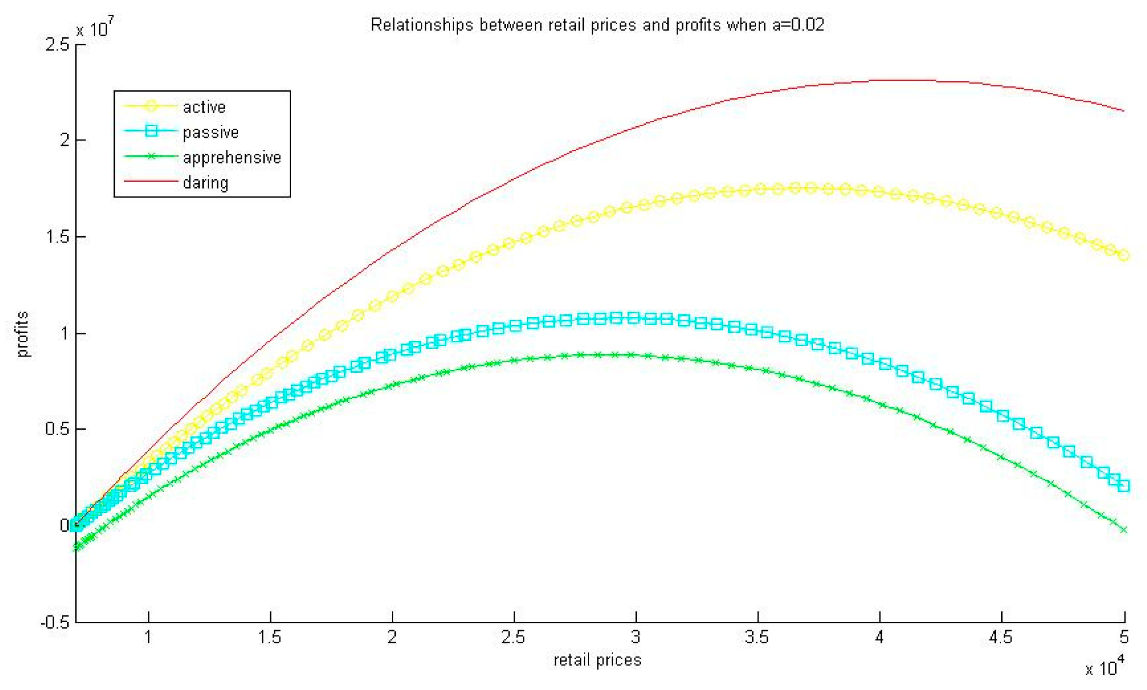
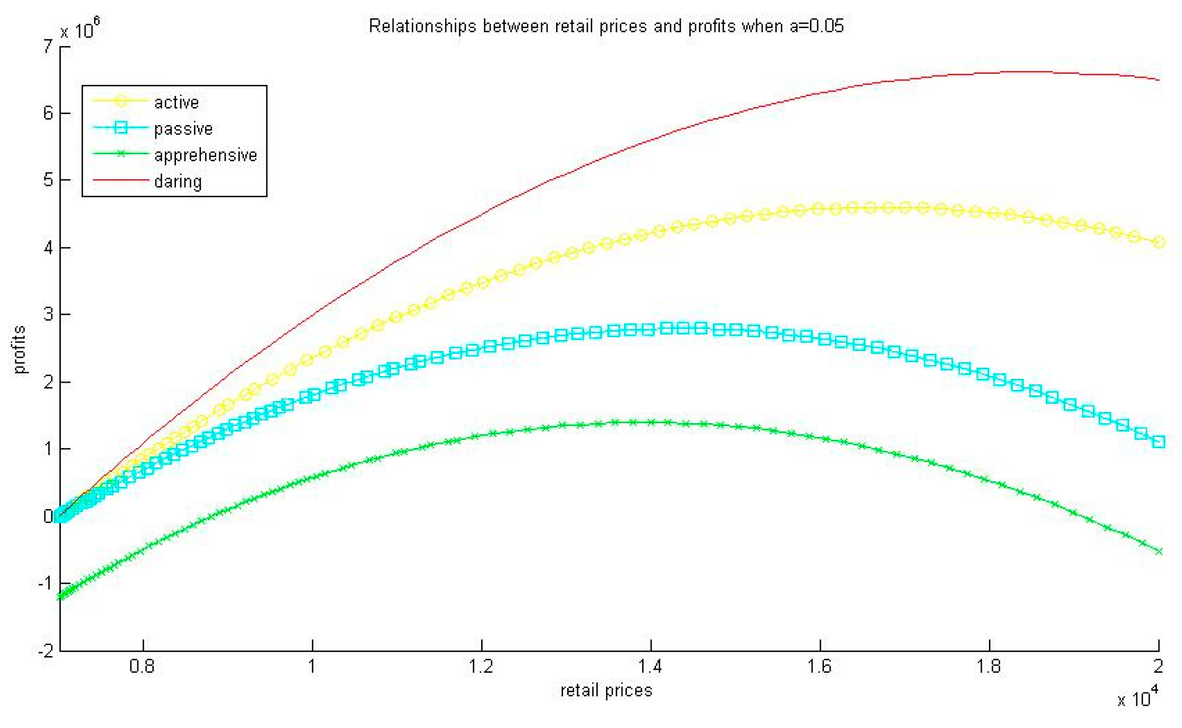
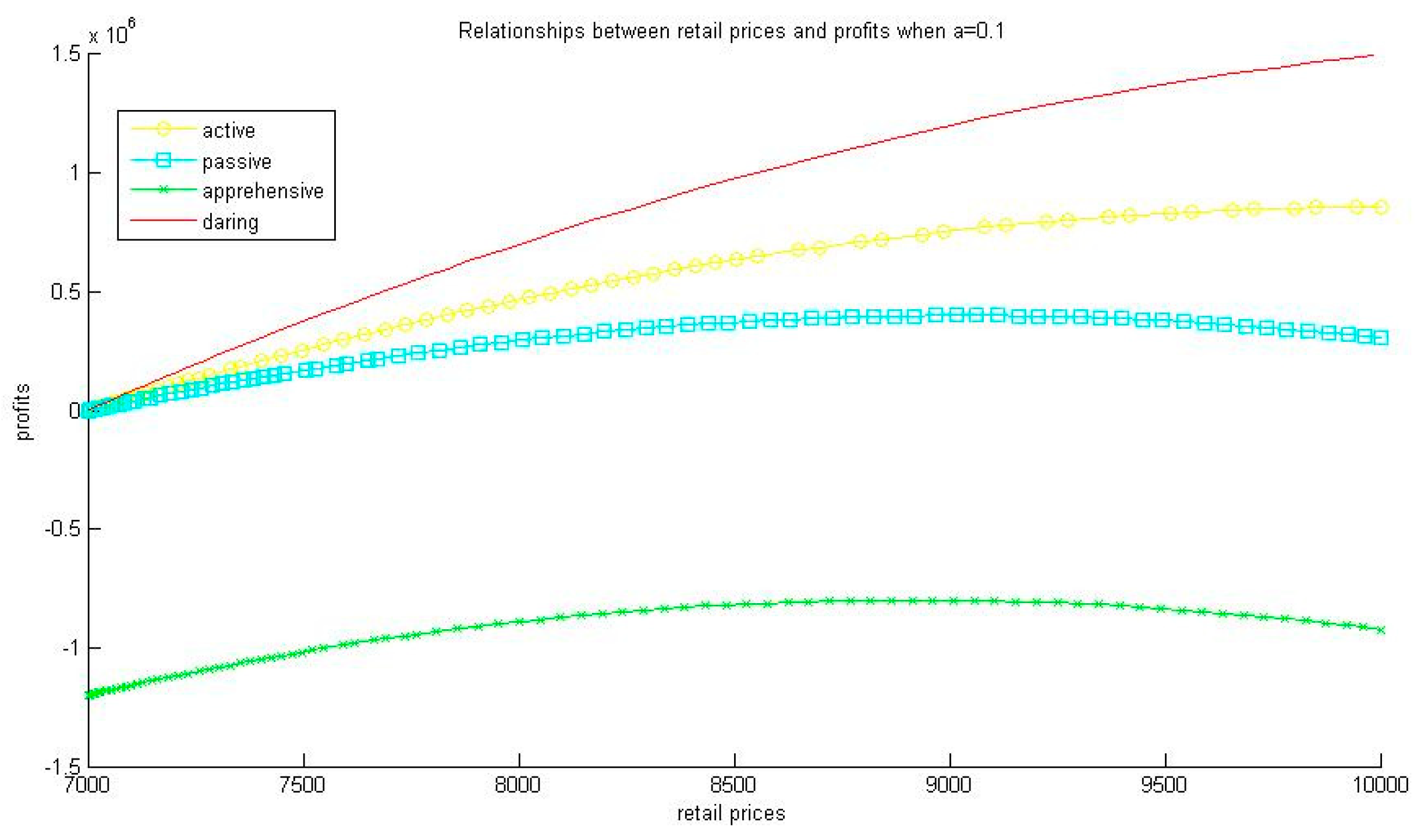
For simplification, the satisfaction function is the normalization of $r(R,b,q)$. We obtain $R_1^{*}=\mathrm{16,767}$, $R_2^{*}=\mathrm{14,328}$, $R_3^{*}=\mathrm{13,919}$ and $R_4^{*}=\mathrm{18,500}$; $r_1^{*}=\mathrm{459,800}$, $r_2^{*}=\mathrm{2,792,900}$, $r_3^{*}=\mathrm{1,394,500}$ and $r_4^{*}=\mathrm{6,612,500}$. Similarly, we can obtain that when $a=0.02$, $R_1^{*}=\mathrm{36,804}$, $R_2^{*}=\mathrm{29,384}$, $R_3^{*}=\mathrm{28,797}$, $R_4^{*}=\mathrm{41,000}$, $r_1^{*}=\mathrm{17,507,000}$, $r_2^{*}=\mathrm{10,766,000}$, $r_3^{*}=\mathrm{8,865,800}$ and $r_4^{*}=\mathrm{23,120,000}$; when $a=0.10$, $R_1^{*}=\mathrm{10,000}$, $R_2^{*}=9033$, $R_3^{*}=8922$, $R_4^{*}=\mathrm{10,000}$, $r_1^{*}=\mathrm{857,140}$, $r_2^{*}=\mathrm{400,110}$, $r_3^{*}=-\mathrm{799,350}$ and $R_4^{*}=\mathrm{1,500,000}$. The relationships between retail prices and profits when $a=0.02$, $a=0.05$ and $a=0.10$ are shown in Figure 1, Figure 2 and Figure 3, respectively.

The numerical example shows three interesting phenomena. First, we observe that with the increasing of market demand’s price sensitivity (the increase of parameter $a$), all of the four types of manufacturers charge the lower retail prices. Second, the numerical example indicates that for any $R>W$, $r_4(R)>r_1(R)>r_2(R)>r_3(R)$. That is the focused profits of the daring manufacturer are higher than the ones of active one; the focused profits of the active manufacturer are higher than the ones of the passive manufacturer; the focused profits of the passive manufacturer are higher than the ones of the apprehensive manufacturer. Third, we have $R_4^{*}>R_1^{*}>R_2^{*}>R_3^{*}$ which shows that the daring manufacturer has the highest optimal retail price; the active manufacturer has a higher optimal price than the passive manufacturer, and the apprehensive manufacturer has the lowest optimal retail price. The first result is similar to Reference [11], however, since we model the behaviors of different types of manufacturers, the second and third results are original. Such conclusions are in accordance with phenomena in the real business world.

6. Conclusions

Considering the one-time feature of the manufacturer’s decision-making for producing and pricing the innovative product in a monopoly market, we propose the price-setting newsvendor model for an innovative product with the OSDT. Unlike the price-setting newsvendor model with the EU where the optimal retail price and production quantity are obtained based on the weighted average of all possible payoffs’ utilities, the price-setting newsvendor model with OSDT determines the optimal retail price and production quantity based on the satisfaction level of its focus point (scenario). Clearly, the proposed model is scenario-based, which is radically different from the lottery-based models.

Active, passive, apprehensive and daring manufacturers are considered in this research. If the profit functions are concave, we have the following conclusions:

The daring manufacturer always imagines a higher profit than the active manufacturer; meanwhile, the active manufacturer imagines higher than a passive manufacturer, and the passive manufacturer imagines higher than an apprehensive manufacturer.

The daring manufacturer has the highest optimal retail price; the active manufacturer has a higher optimal price than the passive manufacturer, and the apprehensive manufacturer has the lowest optimal retail price.

Whichever the manufacturer’s type is, decreasing the price sensitivity of the demand is efficient for charging a high retail price in the innovative product market.

Such theoretical results are consistent with the phenomena in the real business world and provide managerial insights into different types of manufacturer’s behaviors in a monopoly market. Using the obtained analytic results, several phenomena in the luxury goods market have been well explained. In the near future, we will analyze the channel coordination and personality information sharing in the supply chain.

References

- Cachon, G.P. Supply chain coordination with contracts. In Handbooks in Operations Research and Management Science: Supply Chain Management; Graves, S.C., De Kok, A.G., Eds.; Elsevier: Amsterdam, The Netherlands, 2003; Volume 11, pp. 229–339. [Google Scholar]
- Chen, J.; Bell, P. The impact of customer returns on decisions in a newsvendor problem with and without buyback policies. Int. Trans. Oper. Res. 2011, 18, 473–491. [Google Scholar] [CrossRef]
- Liu, X.; Chan, F.T.S.; Xu, X. Hedging risks in the loss-averse newsvendor problem with backlogging. Mathematics 2019, 7, 429. [Google Scholar] [CrossRef]
- Petruzzi, N.C.; Dada, M. Pricing and the newsvendor problem: A review with extensions. Oper. Res. 1999, 47, 183–194. [Google Scholar] [CrossRef]
- Qin, Y.; Wang, R.; Vakharia, A.J.; Chen, Y.; Seref, M.M.H. The newsvendor problem: Review and directions for future research. Eur. J. Oper. Res. 2011, 213, 361–374. [Google Scholar] [CrossRef] [Green Version]
- Petruzzi, N.C.; Dada, M. Newsvendor models. In Wiley Encyclopedia of Operations Research and Management Science; Cochran, J.J., Cox, L.A., Keskinocak, P., Kharoufeh, J.P., Smith, J.C., Eds.; John Wiley & Sons: Hoboken, NJ, USA, 2010; pp. 3528–3537. [Google Scholar]
- Chen, X.; Pang, Z.; Pan, L. Coordinating inventory control and pricing strategies for perishable products. Oper. Res. 2014, 62, 284–300. [Google Scholar] [CrossRef]
- Chen, X.; Simchi-Levi, D. Coordinating inventory control and pricing strategies with random demand and fixed ordering cost: The finite horizon case. Oper. Res. 2004, 52, 887–896. [Google Scholar] [CrossRef]
- Kocabiyikoglu, A.; Popescu, I. An elasticity approach to the newsvendor with price-sensitive demand. Oper. Res. 2011, 59, 301–312. [Google Scholar] [CrossRef]
- Lu, Y.; Simchi-Levi, D. On the unimodality of the profit function of the pricing newsvendor. Prod. Oper. Manag. 2013, 22, 615–625. [Google Scholar] [CrossRef]
- Raz, G.; Porteus, E.L. A fractiles perspective to the joint price/quantity newsvendor model. Manag. Sci. 2006, 52, 1764–1777. [Google Scholar] [CrossRef]
- Salinger, M.; Ampudia, M. Simple economics of the price-setting newsvendor problem. Manag. Sci. 2011, 57, 1996–1998. [Google Scholar] [CrossRef]
- Xu, M.; Lu, Y. The effect of supply uncertainty in price-setting newsvendor models. Eur. J. Oper. Res. 2013, 227, 423–433. [Google Scholar] [CrossRef]
- Xu, X.; Cai, X.; Chen, Y. Unimodality of price-setting newsvendor’s objective function with multiplicative demand and its applications. Int. J. Prod. Econ. 2011, 133, 653–661. [Google Scholar] [CrossRef]
- Fisher, M.L. What is the right supply chain for your product? Harv. Bus. Rev. 1997, 75, 105–116. [Google Scholar]
- Guo, P. One-shot decision theory. IEEE Trans. SMC Part A Syst. Hum. 2011, 41, 917–926. [Google Scholar] [CrossRef]
- Guo, P. One-shot decision approach and its application to duopoly market. Int. J. Inf. Decis. Sci. 2010, 2, 213–232. [Google Scholar] [CrossRef]
- Guo, P. Private real estate investment analysis within a one-shot decision framework. Int. Real Estate Rev. 2010, 13, 238–260. [Google Scholar]
- Guo, P. One-shot decision theory: A fundamental alternative for decision under uncertainty. In Human-Centric Decision-Making Models for Social Sciences; Studies in Computational Intelligence 502; Guo, P., Pedrycz, W., Eds.; Springer: Berlin/Heidelberg, Germany, 2014; pp. 33–55. [Google Scholar]
- Guo, P.; Li, Y. Approaches to multistage one-shot decision making. Eur. J. Oper. Res. 2014, 236, 612–623. [Google Scholar] [CrossRef]
- Guo, P.; Yan, R.; Wang, J. Duopoly market analysis within one-shot decision framework with asymmetric possibilistic information. Int. J. Comput. Intell. Syst. 2010, 3, 786–796. [Google Scholar] [CrossRef]
- Li, Y.; Guo, P. Possibilistic individual multi-period consumption–investment models. Fuzzy Sets Syst. 2015, 274, 47–61. [Google Scholar] [CrossRef]
- Wang, C.; Guo, P. Behavioral models for first-price sealed-bid auctions with the one-shot decision theory. Eur. J. Oper. Res. 2017, 261, 994–1000. [Google Scholar] [CrossRef]
- Guo, P.; Ma, X. Newsvendor models for innovative products with one-shot decision theory. Eur. J. Oper. Res. 2014, 239, 523–536. [Google Scholar] [CrossRef] [Green Version]
- Zhu, X.; Guo, P. Approaches to four types of bilevel programming problems with nonconvex nonsmooth lower level programs and their applications to newsvendor problems. Math. Methods Oper. Res. 2017, 86, 255–275. [Google Scholar] [CrossRef]
- Zhu, X.; Guo, P. Bilevel programming approaches to production planning for multiple products with short life cycles. 4OR Q. J. Oper. Res. 2019, 1–25. [Google Scholar] [CrossRef]
- Guo, P. Focus theory of choice and its application to resolving the St. Petersburg, Allais, and Ellsberg paradoxes and other anomalies. Eur. J. Oper. Res. 2019, 276, 1034–1043. [Google Scholar] [CrossRef]
- Guo, P.; Zhu, X. Focus Programming: A Fundamental Alternative for Stochastic Optimization Problems. 2019. Available online: https://ssrn.com/abstract=3334211 (accessed on 29 August 2019).
- Gavirneni, S.; Isen, A.M. Anatomy of a newsvendor decision: Observations from a verbal protocol analysis. Prod. Oper. Manag. 2010, 19, 453–462. [Google Scholar] [CrossRef]
- Wan, W.; Liu, L. iPhone 6s being sold for insane amounts of money in China. The Washington Post. 22 September 2014. Available online: http://allyourmobiles.blogspot.com/2014/09/iphone-6s-being-sold-for-insane-amounts.html (accessed on 29 August 2019).
- Cachon, G.P. What is interesting in operations management? Manuf. Serv. Oper. Manag. 2012, 14, 166–169. [Google Scholar] [CrossRef]
- Grothaus, M. Meeting Hong Kong’s Obnoxious iPhone Scalpers. Vice. 27 October 2014. Available online: https://www.vice.com/da/article/8gdeea/meeting-hong-kongs-obnoxious-iphone-scalpers-283 (accessed on 29 August 2019).
- Kapner, S.; Passariello, C. Soaring luxury-goods prices test wealthy’s will to pay. The Wall Street Journal. 2 March 2014. Available online: https://www.wsj.com/articles/soaring-luxury-goods-prices-test-wealthys-will-to-pay-1393803469 (accessed on 29 August 2019).
- Jacobson, T.; Florio, R.; Salvador, T. The premium of value pricing and promoting luxury to the new consumer. Accenture. 19 January 2011. Available online: https://www.accenture.com/us-en/~/media/accenture/conversion-assets/dotcom/documents/global/pdf/strategy_4/accenture-the-premium-of-value.pdf (accessed on 29 August 2019).
Figure 1.
Relationships between retail prices and profits when .
Figure 2.
Figure 3.