A New Vision on the Prosumers Energy Surplus Trading Considering Smart Peer-to-Peer Contracts

Abstract

A growing number of households benefit from government subsidies to install renewable generation facilities such as PV panels, used to gain independence from the grid and provide cheap energy. In the Romanian electricity market, these prosumers can sell their generation surplus only at regulated prices, back to the grid. A way to increase the number of prosumers is to allow them to make higher profit by selling this surplus back into the local network. This would also be an advantage for the consumers, who could pay less for electricity exempt from network tariffs and benefit from lower prices resulting from the competition between prosumers. One way of enabling this type of trade is to use peer-to-peer contracts traded in local markets, run at microgrid (μG) level. This paper presents a new trading platform based on smart peer-to-peer (P2P) contracts for prosumers energy surplus trading in a real local microgrid. Several trading scenarios are proposed, which give the possibility to perform trading based on participants’ locations, instantaneous active power demand, maximum daily energy demand, and the principle of first come first served implemented in an anonymous blockchain trading ledger. The developed scheme is tested on a low-voltage (LV) microgrid model to check its feasibility of deployment in a real network. A comparative analysis between the proposed scenarios, regarding traded quatities and financial benefits is performed.

1. Introduction

In distribution systems, intelligent networks (known as ‘smart grids’) are implemented for encouraging energy savings and the integration of distributed generation sources, to help distribution utilities choose the optimal investment plans, achieve optimal operation of their systems, and to increase system efficiency. Other issues that need to be taken into consideration are the proliferation of prosumers and the creation of new consumer services. These research directions are in agreement with the European Union (EU) priorities, stated in the European Commission (EC) Communication published in 28 November 2018: renewable technologies, which must be the core of the new energy systems, smart grids, better energy efficiency, and low-carbon technologies. The fight against climate change is one of the five main topics of the EU extensive strategy for smart, sustainable and inclusive growth.

A microgrid can be defined as a LV network with loads, distributed energy resources (DER), and energy storage systems (ESS) connected to it, which can be operated in standalone or grid connected mode. The capacity of the DER considered in μG is in relatively small scale, but without universal agreement. It is mentioned as smaller than 100 kW by Huang et al. [1]. One of the main concepts in the active distribution network (ADN) is demand side management (DSM). Demand response (DR) as one of subcategories of DSM is defined by the EC as “voluntary changes by end-consumers of their usual electricity use patterns—in response to market signals”. It is a shift of electricity usage in response to price signals or certain requests [2].

The existing energy management systems (EMS) available to operators will soon seem archaic with the increasing integration of small-scale renewable energy sources (SSRES), distributed generation (DG), ESS, electric vehicles, and DR programs. With the increased penetration of DER into the electricity distribution network (EDN), the power flow no longer remains unidirectional and power system control becomes increasingly complex. With their distributed control, μGs provide a novel alternative and can help transform the existing burdened power system into a smart grid. As a first step towards these goals, in the EU, the implementation of smart metering systems is finished in some countries and is in various levels of development in others [3]. The spread of smart metering allows the creation of the μG energy markets (micro-markets: μM), which enable small-scale participants such as consumers (residential buildings) and prosumers (defined as consumers with excess of produced power) to locally exchange the energy surplus [4].

In addition to the metering functions, smart meters provide a wide range of applications: two-way communication between the smart meters mounted at consumer/prosumers sites and concentrators (management platforms or traders), secure data transmission between the participants, remotely controlled connections on the μGs and specify the limitation of consumers/prosumers, and differentiated time-of-use tariffs [5]. The blockchain concept, as a rising technology, proposes new challenges for the µG based on the decentralized or community energy market, which ensures clear and favorable applications that allow consumers to be prosumers in a secured way [6]. The application of blockchain for μM has recently earned the consideration of the researchers worldwide.

Through bilateral prosumer-consumer contracts, consumers can obtain electricity at significantly lower price offers than from traditional suppliers. If a blockchain trading system is used, transactions are distributed and encrypted for data validation and local storage at the μG level. Each member of the network automatically verifies, confirms, and saves the authenticity of the transaction data. Furthermore, third-party trading agents are not needed, because the trading process is performed by participants, who become witnesses and guarantees for every transaction.

The massive implementation of active μGs will be a critical challenge for electrical grids that will require new management and control strategies. Aggregators and μGs, in a certain manner, may look similar because they were both introduced as aggregation element, which allows a coherent operation of a number of DERs, ESSs and flexible loads. In reality, there is a substantial difference between these two actors. In fact, μG perform the optimal management and control of resources based on geographical contiguity. On the contrary, this characteristic is not required in aggregators and the affiliated resources can be delocalized through the territory.

In Romania, by the provisions of Order 228 of 28 December 2018 proposed by ANRE (Regulation National Agency in Energy Domain) regarding prosumers, consumers who wish to trade the energy produced from renewable sources such as photovoltaic (PV), biomass, wind, cogeneration, etc. on the free market, and taking into account the current economic and technical context from the energy industry regarding the increase of investments in the small sources of distributed generation, it is expected that the need to develop new technological platforms for monitoring, management, and advanced analysis of the energy market will extend to the level of μG and of individual consumers, with the modernization of technical infrastructures and their transformation into smart μG.

According to the aforementioned regulations, the electricity suppliers bound by contracts with prosumers are required to buy the electricity at the weighted average day-ahead market price from the previous year. Thus, the prosumer can sell on the market its electricity generation surplus, while the advantage for the supplier is the exemption from the payment of the distribution network tariff. This trading system is the most basic, limiting the options of both parties, prosumers who want to sell and consumers who want to buy electricity at lower prices.

By not allowing prosumers to set custom selling prices, it does not account for differences in generation costs and installed capacity. The incentive of increasing local generation is not present. Consumers cannot buy electricity directly from the prosumers, and thus do not the freedom to choose specific prosumers for trading.

The aim of this paper is to provide an innovative electricity trading system implementing a new vision for local electricity trading between prosumers and consumers in μGs. In electricity markets, trading is based usually on the minimum selling price principle. However, the electricity quantities traded in μGs are much smaller, with narrower differences between selling prices. Thus, other criteria can become equally relevant, such as traded quantity or distance between seller and buyer. On the other hand, blockchain trading is based on the principle of first came, first served (FCFS), regardless of quantity and price. Based on these considerations, the prosumer electricity surplus trading (PEST) algorithm proposed in this paper offers several transaction priority scenarios, prosumer-driven and consumer-driven. In the prosumer-driven scenarios, the local generators with surplus to sell choose their trading parties (consumers), based on four principles: minimum distance, maximum instantaneous demand, maximum daily demand, and blockchain trading. In the consumer-driven scenario, consumers use the blockchain trading system to place buying offers, which are fulfilled by selling offers in the ascending order of prices. The term “smart” from the title coincide with the mode of transaction priority scenarios, where the peers sign according to its own advantage.

The remainder of the paper is structured as follows. Section 2 presents a literature review on the proposed problem highlighting the advantages of the proposed PEST methodology. Section 3 describes the proposed PEST algorithm for prosumer-consumer trading in μG. In Section 4, a case study is performed, with a comparison between the proposed trading strategies, outlining their particularities. The paper ends with Section 5 and references.

2. Literature Review

The latest trends in academic or industrial research describe several PEST solutions via P2P contracts with or without blockchain technologies. The P2P concept represents a process in which the prosumers trade energy in exchange for a deposit with the consumer [7]. Prosumers use P2P contracts for selling their generation surplus to local consumers, instead of selling it back to the grid.

In active distribution networks, the P2P trading process is structured as a four-layer architectural business model, from which three dimensions are used for secured energy exchange: bidding between prosumers and consumers for certain energy quantities through smart contracts, the selection of the offers to be fulfilled, energy delivery, and finally payment settling. In the aforementioned trading procedure, selling and buying offers are posted in a ledger secured by the blockchain technology. Offers are verified by the system administrator and accepted by parties by signing the P2P contracts. The energy demand can be met by any prosumer, and energy exchange in lieu of digital money takes place [8].

If a μM is established in the μG, small-scale prosumers and consumers have a market platform to trade energy generated locally within their community. In this way, energy losses are reduced, because the consumption of energy is in close proximity to the source. This helps to promote the sustainable and efficient utilization of local resources, because the market participants in a μM do not compulsorily need to be physically connected. Multiple energy producers, prosumers, and consumers can be added to form a local (or virtual) community and the control can be maintained through local (virtual) μGs. Blockchain is a secure system for transactions, which also provides distributed applications to convey an understanding of each block and data on the system [9]. Even though in literature it exists an important number of research papers regarding the μM on the one hand and blockchain technology on the other hand, their aggregation is still lacking [10].

Several P2P transaction mechanisms are known from the literature as follows: based on transaction zoning in [11], based on total share of SSRES between neighbourhoods for energy bills saving in [7,12], and also on the provision of ancillary services and voltage regulation service [13]. P2P energy trading schemes are also proposed for local community or μG which already have implemented the blockchain technologies [14]. In [15], to secure the transactions of the PEST by P2P contracts, a specific blockchain technology is developed. Other authors propose double auction mechanism. The maximization of social welfare in the PEST can use auction-based mechanism [16,17]. The author from [18] uses an optimum pricing scheme for local electricity trading in μGs considering four particular priorities. In other words, the prosumers become the new actors in local electricity power market, considered as μM [19,20]. A different formulation of the PEST optimization follows a hierarchical framework considering the future energy price uncertainty in [21], information and communication technologies (ICT) in [22], and multi-layer architecture model in [23,24]. Paper [25] proposes a comprehensive analysis regarding the P2P communication architectures and highlights the performance of common protocols evaluated in accordance with IEEE 1547.3-2007.

In study [26], a P2P index optimization process was proposed. Here, a compromise regarding the balancing between the demand and generation in the LV network are identified. An incentive mechanism for PEST is presented in [27]. In the aforementioned paper, the authors consider three prices for prosumers profit maximization. Moreover, in [20,21,28], the authors proposed an evolutionary game theory-based approach for a dynamic modelling of the consumers (as buyers), in order to select the prosumers (as sellers). Thus, the evolutionary game theory was used for a dynamic modelling of the buyers for selecting sellers. The particular approach from [29] consider a Model Productive Control (MPC) method, for transactions only between two SSRES (prosumers), to avoid selling the surplus electricity production to classical traders or suppliers. This work considers the direct transactions without P2P contracts and blockchain technologies. Another category of the published papers regards the transactions of the PEST in the context of transactive energy in μGs [30,31,32]. The authors in [33] the transactions consider different preference of prices.

To highlight the newness and the originality of our proposed approach, in

Table 1. A comparative state of the art between our method and the literature.

References	Path of Supply (S1)	Instantaneous Power Demand (S2)	Daily Energy Consumption (S3)	Blockchain Technologies (S4)	Minimum Price for Consumers (S5)	P2P Contracts
[7,17]	no	no	no	no	yes	yes
[11,12,25]	yes	no	no	no	no	yes
[13]	no	no	yes	yes	no	yes
[14,15]	no	no	yes	yes	yes	yes
[16,23]	yes	no	no	yes	no	yes
[18]	no	no	yes	no	no	no
[20,26]	no	no	yes	no	no	yes
[21,22,30]	no	no	no	no	yes	no
[27]	no	no	no	yes	yes	no
[28]	no	no	yes	no	yes	yes
[29]	no	yes	no	no	no	yes
[31]	no	yes	no	yes	no	no
[32,33]	no	no	no	no	yes	yes
Proposed approach	yes	yes	yes	yes	yes	yes

, a brief description of the literature paper is presented, considering the five proposed trading objectives (four prosumer-driven and one consumer-driven) and the P2P contracts. The four prosumer-driven are S1: path of supply length, S2: instantaneous power demand, S3: daily energy consumption-based clustering, and S4: blockchain technologies. In addition, the consumer-driven scenario is S5—minimum price for consumers. It should be mentioned that many papers are the same with the References [7,11,12,13,14,15,16,17,18,20,21,22,23,25,26,27,28,29,30,31,32,33] presented in Table 1.

A previous work of the authors, in [34], proposes only at principle level a particular approach for prosumers energy trading in μGs as an efficient P2P exchange based on the blockchain technology. Specifically, the algorithm solves a mathematical model for the latest challenges regarding both the ADN and the newest type of electricity market participants (prosumers) using virtual or crypto price as the transaction currency. In other words, this work emphasizes the capabilities and plausible benefits of P2P contracts for energy trading in local μGs from both prosumers and consumers perspectives. Taking into account that the Smart Meters are able to perform automatic energy transfer from the prosumers to the μG, the energy exchanged between the μGs peers, the utilities will be reduced, trough the minimization of active power losses. In the aforementioned context, the proposed algorithm implemented in the MATLAB environment is developed as a final energy market transaction platform for both the prosumers and traders.

3. A New Vision for Prosumer Energy Surplus Trading Algorithm

As described in the previous sections, an increasing number of consumers from LV EDN are using SSRES such as PV panels and wind turbines to gain energy independence by reducing the electricity need from the classic grid. This trend is driven by incentives provided by governments, such as subsidies for installing equipment or legislative provisions that allow them to sell the generation surplus back to the grid or to other consumers, thus becoming prosumers. The trading model that gives prosumers the ability to sell the surplus generation to the grid uses often-regulated tariffs, which results in low profits. The financial gain of the prosumers can increase if they get the possibility to sell energy to the consumers from their vicinity, at negotiated prices, via new trading tools, such as P2P contracts. Furthermore, to ensure equal access and transaction anonymity, the blockchain technology can be implemented to secure prosumer-consumer transactions.

The paper presents an algorithm for electricity transactions between prosumers and consumers belonging to the same local network or μG, using P2P contracts and, optionally, the blockchain technology.

In this section, prosumers and consumers’ selection process, P2P pricing methodology, and the surplus trading mathematical model will be explained in detail.

The trading model implemented in the algorithm uses the following assumptions:

• Transactions are settled by the local non-profit μG manager or aggregator using the consumer or prosumer merit order derived from the priority mechanism agreed for trading and data from the metering system.
• The prosumer-consumer acquisition priority rules are the same for the entire μG.
• To be able to acquire electricity from a prosumer Pk, a consumer Cj must have previously signed a P2P contract that includes the bilateral trading agreement, price, and other supplemental information, such as trading priority.
• By default, any prosumer and prosumers in the μG have signed bilateral P2P trading contracts. In other words, any prosumer who has a generation surplus can theoretically sell electricity to any consumer in the microgrid. This setting is changeable to exclude any consumer from the trading process.
• When a consumer is awarded a P2P contract, the power supplied by the prosumer will try to match the entire load of the consumer, within the limit of the available surplus, as in Equation (1). This setting is changeable to allow specified quantity requirements for each consumer.

$$P_{trade,k,j,h}=\{\begin{array}{c}{P}_{j,h},\mathrm{if}{P}_{surplus,k,h}\ge P_{j,h}\\ P_{surplus,k,h},otherwise\end{array}$$

(1)

where P_trade,k,j,h is the power traded at hour h (h = 1, ..., nh), to consumer j (j = 1, ..., nc) by prosumer k (k = 1, ..., np); P_j,h is the own consumption of prosumer k at hour h, and P_surplus,k,h is the power surplus at hour h of the prosumer k.

• The selling price of a prosumer is considered fixed for all trading intervals of a day. This assumption is made because only PV panels are used at this point as generation sources, and no storage capabilities are present in the μG. Thus, the local generation does not cover evening peak load or low consumption night hours, which would favor the application of differentiated tariffs.
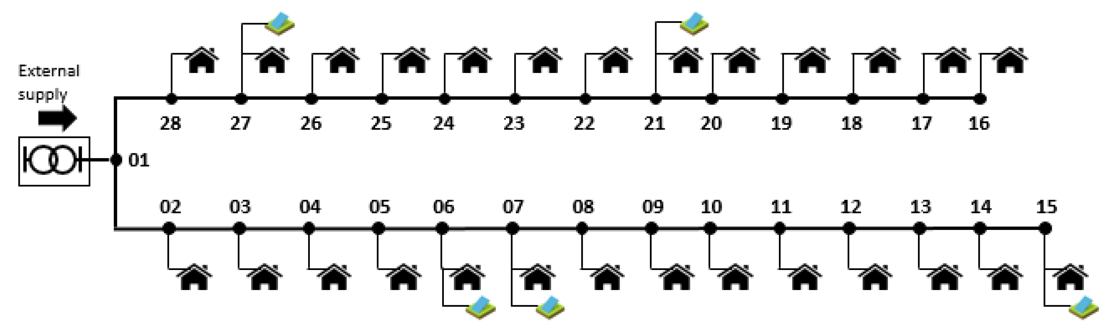
• The consumers in the network are generally one-phase, supplied through a four-wire three-phase network. Prosumers are supplying their surplus generation in the μG using a three-phase balanced connection point, as required by technical regulations for LV distribution systems [35].
• When transactions take place between certain prosumers and consumers, the prosumers will deliver and the consumer will receive electricity from the same grid.
• If the surplus exceeds the local demand traded via P2P contracts, the μG market administrator will sell the untraded electricity back to the grid, at regulated tariffs.

The main input data needed by the algorithm refers to the consumption and local generation available in the μG. For this, two matrices are provided: matrix C = C (h, j) ∈ ℝ^nh×ncfor consumptions and matrix G = G (h, k) ∈ ℝ^nh×np for generation. Generation will be available for prosumers for which, at the same hour h and prosumer k, G (h, k) > C (h, k), and the surplus available for trading follows as:

S (h, k) = G (h, k) − C (h, k)

(2)

computed into a matrix S = S (h, k) ∈ ℝ^nh×np.

Also, for prosumers, the daily selling price is provided as a matrix PR = PR(h, k) ∈ ℝ^nhxnp, where any element PR(h, k) represents the selling price for a generic prosumer k at hour h.

This surplus will be sold to local consumers if P2P contracts exist, or to the grid. The local transactions are governed by a priority of supply mechanism agreed at the μG level, which describes the order in which any consumer Cj can acquire electricity from any prosumer Pk. In the algorithm, the complete list of priorities is encoded in a matrix M_x = M_x(k, j) ∈ ℤ^np×nc. A generic element M_x(k, j) denotes the merit order of consumer j in the priority list of prosumer k, for the trading scenario x.

The trading algorithm proposed in the paper offers improved flexibility by considering two trading paradigms: consumer-driven, where the minimum price for consumers is sought, as in any traditional electricity market, and prosumer-driven, where the aim is to incentivize prosumer offers.

In the prosumer-driven scenarios, trading is performed to prioritize the selling of the generation surplus to consumers. The prosumer selling price is not considered, and the selling offers are fulfilled using the FCFS principle [34]. When trading is consumer-driven, the fulfillment of the consumer needs is sought first, and the prosumers with the lowest selling prices are prioritized for trading, as shown in Figure 1.

Five scenarios for assigning consumer priorities for P2P trading are available:

• Prosumer-driven

  ○

  Scenario 1: Path of supply length

  ○

  Scenario 2: Instantaneous power demand

  ○

  Scenario 3: Daily energy consumption-based clustering

  ○

  Scenario 4: Blockchain offers

• Consumer-driven:

  ○

  Scenario 5: Minimum price for consumers

In each scenario, when the primary priorities are equal, a second dissociation criterion is applied. A description of these scenarios follows.

3.1. Trading Priority Based on the Length of the Supply Path—Scenario 1 (Prosumer-Driven)

If this criterion is used, the prosumers will sell their electricity surplus to consumers using as ranking criterion the minimal network length between the generation and consumption locations. The consumer(s) with minimal network length from a given prosumer will be awarded first its available surplus, followed by other consumers in the ascending order of the connection distance. If two consumers are located at equal network lengths from a prosumer, the one with the higher power request will be preferred:

$$\begin{gathered} \mathrm{Priority}\mathrm{level}1\min (L_{j,k}) \\ \mathrm{Priority}\mathrm{level}2\max ({\mathrm{P}}_{h,j}) \end{gathered}$$

(3)

This prioritization approach is modelling the true load flows occurring in an EDN, where the energy generated locally would predominantly supply the consumptions located at the closest locations, following the shortest path. Thus, the consumers most likely to physically receive the surplus are preferred for trading in this case.

3.2. Trading Priority Based on Consumer Hourly Demand—Scenario 2 (Prosumer-Driven)

In this scenario, the prosumers will sell their electricity surplus to consumers ranked in descending order of their trading offer or instantaneous consumption measured in the trading hour. If two consumers have equal power trading requirements at the same time, the one located closer to the seller prosumer will be preferred:

$$\begin{gathered} \mathrm{Priority}\mathrm{level}1\max ({\mathrm{P}}_{h,j}) \\ \mathrm{Priority}\mathrm{level}2\min (L_{j,k}) \end{gathered}$$

(4)

This prioritization is favoring for trading the consumers with the highest instantaneous demand, reducing the number of contracts fulfilled simultaneously by one prosumer. The use of this prioritization procedure minimizes the number of financial settlements required in each trading interval and in a day. In most cases, if a consumer is accepted for trading, its financial saving resulting from the lower electricity prices offered by prosumers, compared with standard regulated prices, is maximized. Larger profits can act as an incentive for consumers with high demand to be involved in the retail electricity market operated at microgrid level.

3.3. Trading Priority Based on Consumer Daily Demand—Scenario 3

In this scenario, the trading priority considers the total electricity demand of the consumers over 24 h. The consumers prioritized for receiving the prosumers’ surplus will be those with the highest daily demand. For this purpose, the Ward hierarchical clustering method was applied.

The Ward method is an agglomerative hierarchical method that first assigns each observation to its own cluster and then groups adjacent clusters so that minimum variance within a cluster is obtained. The distance between two clusters a and b is computed with:

$$d_{ab}=\frac{{\Vert \overline{c_a}-\overline{c_b}\Vert }^2}{\frac{1}{n_a}+\frac{1}{n_b}}$$

(5)

where: d_ab refers to the distance between cluster a and cluster b, $\overline{c_X}$ is the mean of cluster X, ‖ ‖ is the Euclidean length, and n_x is number of elements grouped in cluster X.

The minimum variance criterion used by the Ward method is grouping the consumers in clusters of similar demand level and pattern over 24 h. In the algorithm, a maximum of five priority levels were considered for grouping, and within the same priority level, the criterion of the maximum instantaneous hourly demand was applied:

$$\begin{gathered} \mathrm{Priority}\mathrm{level}1\max (W_j) \\ \mathrm{Priority}\mathrm{level}2\max ({\mathrm{P}}_{h,j}) \end{gathered}$$

(6)

3.4. Trading Priority Based on the Blockchain Technology—Scenario 4

The blockchain technology allows secure anonymous transactions that are fulfilled on the FCFS principle. This means that prosumers or the market administrator cannot choose the trading partners, and buying offers are fulfilled regardless of quantity and price, based only on the time of placement in the trading system.

The algorithm simulates this scenario by assigning randomly generated priorities for each consumer and prosumer, at each trading interval. In addition, as a rule, no two consumers can have equal trading priorities, as the time index of each offer is unique in the blockchain system. Thus, no second ranking criterion is required in this case.

3.5. Trading Priority Based on the Minimum Price for Consumers—Scenario 5

A standard market procedure is to accept trading offers based on the minimum selling price. This approach is modeled in the last scenario implemented in the algorithm, where consumers will acquire the electricity from prosumers in the ascending order of the selling process. The consumer offers will be fulfilled in the sequence taken from the blockchain system ledger, on the FCFS principle. If two prosumers have the same price offer, the highest traded quantity will be preferred.

$$\begin{gathered} \mathrm{Priority}\mathrm{level}1\min (\mathrm{P}{\mathrm{R}}_{k,h}) \\ \mathrm{Priority}\mathrm{level}2\max ({\mathrm{P}}_{k,j}) \end{gathered}$$

(7)

Scenarios 1 and 2 require the knowledge of the length of the supply paths from each prosumer to each consumer. Based on these distances, the priority matrix M₁ = M₁ (k, j) ∈ ℤ^np×nc is determined, where a generic element M₁ (k, j) denotes the trading priority of consumer j for prosumer k. Priorities are positive integer numbers. Lower distances between prosumer k and consumer j result in higher trading priority between the two peers. The highest priority level is 1.

Similarly, Scenario 3 requires the priority matrix M₂ = M₂ (k, j) ∈ ℤ^np×nc where each element M₂ (k, j) denotes the trading priority of consumer j for prosumer k determined by the Ward clustering of consumers according to the daily energy demand. Higher demand is equivalent with higher priority.

Scenarios 4 and 5 use the priority matrix M₃ = M₃ (k, j, h) ∈ ℤ^np×ncxnh, where each element M₃ (k, j, h) is the priority of consumer j for prosumer k at hour h, determined by the time index at which consumer j inputs its purchasing offer for hour h. An earlier time index is equivalent with higher priority. In all priority matrices, the highest priority level is 1. A higher value denotes a lower priority.

For the prosumer-driven scenarios, the surplus is computed using Equation (2) for each prosumer. Then, for each hour and prosumer, if the surplus exists, it is distributed to the consumers using one of the priorities from Scn₁ ÷ Scn₄. For the consumer-driven scenario (Scn₅), at each hour h where surplus exists, it is distributed amongst the consumers using the priority determined by the blockchain system, prioritizing the prosumers with the lowest prices.

The results are stored in an acquisition matrix A = A (h, j, k) ∈ ℤ^{nh × nc x np}, where each element A (h, j, k) represents the electricity sold at hour h to consumer j by prosumer k. Similarly, the financial settlement matrix F = F (h, j, k) ∈ ℤ^{nh × nc x np} is computed, where each element F (h, j, k) represents the payment made by consumer j to prosumer k at hour h. The mathematical model used in determining the hourly surplus sold by prosumers to local consumers via a P2P contract is presented in Algorithm 1. Algorithm 1 uses Subroutine 1, Subroutine 2 and Subroutine 3.

Algorithm 1: The proposed trading algorithm

Step 1. Specify trading scenario: 1—network length; 2—instantaneous demand; 3—daily demand; 4—blockchain trading; 5—prosumer minimum price with blockchain. Step 2. Load input data: the consumer load profile matrix C, the prosumer generation matrix G, the supply path lengths of the network, the prosumer price matrix PR. Step 3. According to the selected scenario, compute priority matrices M1, M2, M3. Step 4. Initialize the acquisition matrix A and financial settlement matrix F. Step 5. Initialize the unsold surplus us = 0. Step 6. Trading: for prosumer-driven scenarios for each hour h, h = 1..24 for each prosumer k, k = 1, …, np compute surplus S (h, k); if S (h, k) > 0 srp = S (h, k); find ix, the row index corresponding to prosumer k in matrix M1 case Scenario 1—network length build a temporary consumer priority matrix MTC with two rows:     row 1: line ix from matrix M1;     row 2: line h from matrix C; (MTC, A, F, srp) = Subroutine 1 (MTC, A, F, srp, h, ix, nc). case Scenario 2—instantaneous demand build a temporary consumer priority matrix MTC with two rows:     row 1: line h from matrix C;     row 2: line ix from matrix M1; (MTC, A, F, srp) = Subroutine 2 (MTC, A, F, srp, h, ix, nc) case Scenario 3—daily demand build a temporary consumer priority matrix MTC with two rows:     row 1: line ix from matrix M2;     row 2: line h from matrix C; (MTC, A, F, srp) = Subroutine 1 (MTC, A, F, srp, h, ix, nc) case Scenario 4—blockchain trading build a temporary consumer priority matrix MTC with two rows:     row 1: line ix from matrix M3;     row 2: line h from matrix C; (MTC, A, F, srp) = Subroutine 1 (MTC, A, F, srp, h, ix, nc) Update line h from C using the modified matrix MTC Update the unsold surplus: us = us + srp; for consumer-driven scenarios—prosumer minimum price with blockchain for each hour h, h = 1, …, 24 compute the total surplus for hour h, srph; if srph > 0 build a temporary consumer priority matrix MTC with two rows:     row 1: line h from matrix M3;     row 2: line h from matrix C; build a temporary prosumer priority matrix MTP with two rows:     row 1: line h from matrix PR;     row 2: line h from matrix S; (MTC, MTP, A, F, srp) = Subroutine 3 (MTC, MTP, A, F, h) Step 7. Compute the hourly and total electricity sold by prosumers to each consumer and the electricity traded hourly and daily by all prosumers, using matrices A and F.

Subroutine 1

Step 1. Read input data: the priority matrix MTC, acquisition matrix A, the financial settlement matrix F, the surplus to be distributed between consumers srp, the current prosumer index ix, the current hour h. Step 2. Transpose matrix MTC into matrix MC. Step 3. Sort matrix MC ascending by column 1, and for equal values in column 1, sort descending the corresponding values in column 2. Step 4. Distribute the surplus srp: set initial consumer index: k = 0; while srp > 0 or (k < nc) k = k + 1; if the consumer has a P2P contract subtract the available surplus from its trading offer MC (k, 2) = MC (k, 2) − srp; if the surplus exceeds the consumer contract quantity: MC (k, 2) < 0 update remaining surplus: srp = − MC (k, 2); the contract from consumer k is fulfilled: MC (k, 2) = 0; else the contract from consumer k is partially fulfilled and the surplus is depleted: srp = 0; update matrix MTC for by subtracting from the served consumer demand the fulfilled contract; update acquisition matrix A for hour h according to the served consumer k, serving prosumer ix and traded quantity

Subroutine 2

Step 1. Read input data: the priority matrix MTC, the acquisition matrix A, the financial settlement matrix F, the surplus to be distributed between consumers srp, the current prosumer index ix, the number of consumers nc, the current hour h. Step 2. Transpose matrix MTC into matrix MC. Step 3. Sort matrix MC descending by column 1, and for equal values in column 1, sort ascending the corresponding values in column 2. Step 4. Distribute the surplus srp: set initial consumer index: k = 0; while srp > 0 or (k < nc) k = k + 1; if the consumer has a P2P contract subtract the available surplus from its trading offer MC (k, 1) = MC (k, 1) − srp; if the surplus exceeds the consumer contract quantity: MC (k, 1) < 0 update remaining surplus: srp = − MC (k, 1); the contract from consumer k is fulfilled: MC (k, 1) = 0; else the contract from consumer k is partially fulfilled and the surplus is depleted: srp = 0; update matrix MTC for by subtracting from the served consumer demand the fulfilled contract; update acquisition matrix A and financial settlement matrix F for hour h according to the served consumer k, serving prosumer ix and traded quantity.

Subroutine 3

Step 1. Read input data: the priority matrix for consumers MTC, the priority matrix for prosumers MTP, the acquisition matrix A, the financial settlement matrix F, hour h. Step 2. Transpose matrix MTC into matrix MC, and matrix MTP into matrix MP Step 3. Sort matrix MC in ascending order of consumer priority (column 1). Keep original consumer order in vector idxk. Step 4. Sort matrix MT ascending by column 1, and for equal values in column 1, sort descending the corresponding values in column 2. Keep original prosumer order in vector idxp. Step 5. Compute the total surplus and consumption (st, ct). Step 6. Distribute the surplus srp: set initial consumer index: kc = 0 and prosumer index kp = 0; while (st > 0) & (ct > 0) increase consumer index: kc = kc + 1; read consumption to be traded c_crt = MC (kc, 2); if c_crt > 0, if consumption exists while (c_crt > 0) & (st > 0) increase consumer index: kp = kp + 1; read prosumer surplus p_crt = MP (kp, 2); if p_crt > 0 subtract the surplus from the consumption c_crt = c_crt − p_crt; if the surplus exceeds the consumer contract quantity: c_crt < 0 update remaining surplus: t_crt = c_crt; p_crt = − c_crt; the contract from consumer k is fulfilled c_crt = 0; else the contract from consumer k is partially fulfilled and the surplus is depleted: p_crt = 0; compute traded consumption ctz = abs (t_crt − abs (c_crt); update transposed consumption and generation priority matrices MC (kc, 2) = c_crt; MP (kp, 2) = p_crt; update consumption and generation priority matrices MTC (2, idxc (kc)) = MC (kc, 2); MTP (2, idxp (kp)) = MP (kp, 2); identify price pr = MP (kp, 1); update st and ct; update acquisition matrix A and financial settlement matrix F.

4. Results

The proposed algorithm was tested on a real 0.4 kV EDN from the northeastern Romania. The network, whose one-line diagram is given in Figure 2, supplies 27 one-phase residential consumers using four-wire three-phase overhead lines, mounted on concrete poles. The distance between poles is of 40 m in average.

This network is modeling a μG in which the prosumers located at buses 6, 7, 15, 21, and 27 want to sell their electricity surplus to other consumers. The case study considers that all the consumers in the μG are integrated in the local μM and can receive electricity from the prosumers through P2P contracts. The consumption and generation of the consumers and prosumers are modelled as 24-h profiles taken from the Smart Metering system installed in the μG. The consumption and generation profiles are provided in

Table A1. Active load curve for the 28-bus network, in kW.

-	C2	C3	C4	C5	C6	C7	C8	C9	C10
h1	0.616	2.010	0.273	0.000	1.370	2.418	1.152	1.936	0.310
h2	0.608	1.908	0.078	0.020	1.520	2.210	1.664	1.368	0.678
h3	0.557	2.004	0.048	0.260	1.910	2.149	2.056	1.376	0.300
h4	0.522	2.010	0.306	0.040	1.770	2.151	2.048	2.048	0.640
h5	0.522	1.902	0.063	0.050	1.990	2.192	1.816	1.528	0.360
h6	0.571	2.004	0.165	0.250	2.070	2.299	1.168	2.992	0.468
h7	0.529	1.836	0.213	0.125	2.280	2.364	0.720	3.352	0.748
h8	0.592	1.236	0.060	4.710	2.530	2.543	1.704	2.240	3.208
h9	0.562	1.302	0.312	1.290	1.850	2.382	1.976	2.112	2.815
h10	0.616	1.200	0.258	0.525	1.850	2.549	1.944	2.192	1.483
h11	0.860	1.188	0.243	2.985	1.460	2.426	1.904	2.232	4.538
h12	0.535	1.146	0.423	1.895	1.180	2.414	1.872	2.144	3.295
h13	0.641	1.140	0.198	4.595	1.650	2.450	2.456	2.048	3.650
h14	0.322	1.374	0.378	0.930	1.950	2.418	2.632	2.176	5.230
h15	0.181	1.944	0.321	0.260	1.810	2.444	1.896	2.256	4.293
h16	0.214	1.542	0.207	0.535	2.640	2.467	2.072	2.328	3.895
h17	0.781	2.148	0.495	2.125	2.810	2.553	2.080	2.288	3.028
h18	0.764	1.902	0.282	1.025	2.720	2.757	2.016	2.336	1.980
h19	0.426	1.968	0.336	0.140	3.580	3.042	2.720	2.464	1.768
h20	0.426	1.968	0.336	0.140	3.580	3.042	2.720	2.464	1.768
h21	0.496	1.956	0.207	0.210	5.310	3.515	2.672	3.136	3.033
h22	0.561	1.986	0.405	0.480	5.390	3.248	2.488	1.312	5.695
h23	0.554	1.872	0.246	0.195	4.750	3.075	2.432	1.336	4.033
h24	0.578	1.986	0.045	0.100	3.170	2.713	2.088	1.184	1.180
-	C11	C12	C13	C14	C15	C16	C17	C18	C19
h1	0.230	0.585	0.142	0.910	2.783	2.220	0.210	0.360	0.345
h2	0.220	0.765	0.078	0.920	2.411	1.320	0.000	0.525	0.286
h3	0.200	0.585	0.352	0.925	2.548	0.942	0.000	0.534	0.243
h4	0.200	0.675	0.440	1.225	2.313	0.972	0.045	0.636	0.213
h5	0.200	0.660	0.062	1.345	2.288	0.954	0.000	0.444	0.237
h6	1.240	0.570	1.416	1.290	2.426	1.044	0.115	0.462	0.242
h7	1.400	0.900	0.482	1.325	3.239	1.374	0.075	0.477	0.281
h8	1.440	0.630	0.182	1.520	3.798	3.984	0.475	0.450	0.287
h9	1.170	0.765	0.502	1.430	3.097	2.184	0.380	0.504	0.278
h10	1.130	0.645	1.046	1.120	4.371	1.986	0.495	0.579	0.268
h11	1.390	0.555	0.150	1.170	2.994	1.986	1.130	0.573	0.285
h12	1.740	0.630	1.032	1.265	3.763	2.844	0.630	0.498	0.315
h13	1.760	0.615	0.056	1.760	2.999	1.566	0.420	0.600	0.301
h14	1.200	0.570	0.056	2.000	2.759	0.930	0.980	0.540	0.329
h15	0.280	0.750	0.236	1.840	3.807	0.798	0.955	0.357	0.312
h16	0.460	0.555	1.024	1.815	3.317	1.152	0.965	0.423	0.350
h17	3.180	0.825	0.232	2.015	3.214	1.944	0.970	0.588	0.366
h18	2.570	0.780	0.890	2.365	2.940	2.046	0.960	0.570	0.468
h19	2.890	0.780	0.458	2.480	3.445	2.460	1.450	0.678	0.443
h20	2.890	0.780	0.458	2.480	3.445	2.460	1.450	0.678	0.443
h21	3.210	0.630	0.864	2.580	3.278	1.884	1.385	0.753	0.454
h22	3.260	0.570	1.326	2.365	2.475	1.374	1.660	0.621	0.482
h23	2.815	0.720	0.376	2.060	2.073	1.380	1.235	0.750	0.509
h24	1.780	0.570	0.200	1.495	2.769	1.158	0.880	0.390	0.328
-	C20	C21	C22	C23	C24	C25	C26	C27	C28
h1	1.010	0.973	0.636	0.790	0.049	1.266	0.384	0.248	0.006
h2	1.100	1.013	0.484	0.780	0.056	1.194	0.384	0.296	0.000
h3	0.990	0.733	0.448	0.730	0.749	1.056	0.388	0.260	0.000
h4	1.090	0.453	0.460	0.920	1.148	1.032	0.392	0.292	0.000
h5	1.070	0.680	0.520	0.800	1.148	1.014	0.400	0.208	0.000
h6	1.450	0.773	0.512	1.340	1.148	1.020	0.396	0.356	0.048
h7	2.260	0.980	0.428	0.960	1.946	1.122	0.376	0.700	0.035
h8	0.610	1.560	0.368	0.270	1.393	1.116	0.352	0.336	0.038
h9	0.310	1.580	0.408	0.420	1.596	1.110	0.356	0.144	0.000
h10	0.400	1.347	0.408	1.000	2.975	1.110	0.360	0.128	0.001
h11	0.310	1.713	0.668	0.930	1.519	1.242	0.620	0.204	0.019
h12	0.500	1.913	0.412	1.050	2.492	1.260	0.344	0.320	0.127
h13	0.760	3.127	0.344	1.020	1.974	1.266	0.324	0.476	0.014
h14	0.630	2.560	0.428	0.970	1.974	1.260	0.332	0.384	0.005
h15	1.260	1.433	1.068	1.010	2.240	1.206	0.940	0.456	0.061
h16	1.170	2.013	0.424	1.110	2.296	1.134	2.500	0.352	0.022
h17	1.620	4.000	0.448	1.540	1.778	1.140	2.544	2.000	0.020
h18	1.620	1.067	0.468	1.630	1.939	1.260	2.820	0.876	0.057
h19	1.620	1.907	0.436	1.570	1.750	1.296	2.104	1.824	0.000
h20	1.620	1.907	0.436	1.570	1.750	1.296	2.104	1.824	0.000
h21	2.440	2.473	1.092	1.280	1.106	1.212	2.144	0.728	0.102
h22	2.570	2.253	1.484	1.110	1.092	1.194	2.084	0.688	0.103
h23	1.450	1.933	1.364	0.710	1.092	1.194	2.248	0.256	0.133
h24	1.010	1.260	0.880	0.840	0.763	1.176	2.008	0.324	0.036

and A2 from Appendix A.

Table 2. Local generation and consumption, in kWh, and prosumer selling prices, in MU/kWh.

Hour	Bus with Prosumers					Total Surplus	Total Consumption
	6	7	15	21	27
h06	0	0	1.95	1.59	0	3.54	19.91
h07	0	0.26	1.59	1.81	0	3.65	20.96
h08	0	0.70	1.59	1.73	0.67	4.68	26.86
h09	0.74	1.06	2.23	1.75	1.44	7.21	21.78
h10	1.12	1.09	1.30	2.29	1.61	7.41	21.74
h11	1.89	1.40	2.78	2.04	1.66	9.75	26.50
h12	2.33	1.23	1.88	1.82	1.60	8.85	26.45
h13	2.29	1.41	2.83	0.69	1.51	8.73	27.51
h14	1.35	1.39	2.95	1.18	1.37	8.23	25.25
h15	1.18	1.05	1.55	2.03	1.11	6.91	24.46
h16	0	0.41	1.32	0.82	0.56	3.12	26.19
h17	0	0	1.06	0	0	1.06	32.15
h18	0	0	1.16	1.17	0	2.33	30.75
total	10.90	9.99	24.17	18.90	11.51	75.48	330.52
Selling price	0.43	0.40	0.48	0.55	0.43	-	-

presents the electricity surplus available for trading in the considered interval, for all the prosumers. This surplus will be distributed between the consumers or/and prosumers using one of the priority scenarios built in the proposed algorithm, as presented in the previous section.

The electricity price is considered constant for each prosumer over the trading interval, and is also given in Table 2. The regulated price at which consumers can buy electricity from the classic market operator has an average level of 0.72 MU/kWh, including taxes. On the other hand, the regulated price at which prosumers can sell electricity back to the grid is set at 0.235 MU/kWh for 2018 [36,37]. Thus, the selling prices for the local prosumers were set in the [0.40, 0.55] MU/kWh interval. As it can be seen from Table 2 and Figure 3, the local generation amounts to 22.8% from the consumption, in the 06:00–18.00 interval, and the hourly surplus does not exceed the demand in any trading interval. This means that all the local generation will be sold in the local μM, through P2P contracts. The generation surplus from Table 2 will be distributed to the consumers with different priorities, according to each scenario.

Table 3. Consumer trading priorities for Scenarios 1 and 3.

	Prosumer
	Scenario 1					Scenario 3
Cons.	6	7	15	21	27	6	7	15	21	27
1	X	X	X	X	X	X	X	X	X	X
2	4	5	13	8	2	4	4	4	4	4
3	3	4	12	9	3	3	3	3	3	3
4	2	3	11	10	4	5	5	5	5	5
5	1	2	10	11	5	2	2	2	2	2
6	X	1	9	12	6	X	1	1	1	1
7	1	X	8	13	7	1	X	1	1	1
8	2	1	7	14	8	3	3	3	3	3
9	3	2	6	15	9	3	3	3	3	3
10	4	3	5	16	10	1	1	1	1	1
11	5	4	4	17	11	3	3	3	3	3
12	6	5	3	18	12	4	4	4	4	4
13	7	6	2	19	13	4	4	4	4	4
14	8	7	1	20	14	3	3	3	3	3
15	9	8	X	21	15	1	1	X	1	1
16	17	18	26	5	11	2	2	2	2	2
17	16	17	25	4	10	4	4	4	4	4
18	15	16	24	3	9	4	4	4	4	4
19	14	15	23	2	8	5	5	5	5	5
20	13	14	22	1	7	3	3	3	3	3
21	12	13	21	X	6	2	2	2	X	2
22	11	12	20	1	5	4	4	4	4	4
23	10	11	19	2	4	4	4	4	4	4
24	9	10	18	3	3	3	3	3	3	3
25	8	9	17	4	2	4	4	4	4	4
26	7	8	16	5	1	3	3	3	3	3
27	6	7	15	6	X	4	4	4	4	X
28	5	6	14	7	1	5	5	5	5	5

presents the priorities computed according to the distance between prosumers and consumers (Scenario 1) and daily energy demand (Scenario 3). For Scenario 1, the priorities are straightforward, the consumers close to the prosumer having maximum trading priority. For instance, if prosumer 21 is used as reference, consumers 22 and 20 will have maximum trading priority, while consumer 14 or prosumer 15 (in case of deficit) will be the last in the priority list. In all scenarios, consumers or prosumers marked with X in Table 3 are excluded from trading. Bus 1 has no load, and each prosumer cannot sell to itself, because it is considered that it is selling on the market its surplus.

The priorities for Scenario 2 are computed in the same manner, but using the hourly demand values indicated in Table A1 from Appendix A as ranking criterion, instead of distance.

For Scenario 3 (daily consumption), the Ward clustering method was run for the consumptions from Appendix A. The dendogram and the clusters obtained after grouping are presented in Figure 4 and Figure 5, which show multiple consumers belonging to the same priority group (with consumers/prosumers 6, 7, 10 and 15 priority group 1). In this case, instantaneous consumption is used for sorting entities belonging to the same group.

The first three scenarios use the same priority for all trading intervals. On the other hand, Scenarios 4 and 5, modelling the blockchain trading priority, require different priorities for each consumer and each hour. Thus, the priority matrix will consider a 28-line, 24-column array for each column in Table 3.

Scenarios 1–4, prosumer-oriented, do not take into account prosumer prices. The prosumer priority order is preset, to take into account the incentivization of specific prosumers, based on criteria particular to each μG, such as date of connection, generation technology, common agreement or maximization of the social welfare. For convenience, the results presented in the following subparagraphs use the bus index as prioritization index, but the algorithm can consider any user-preferred priority.

Scenario 5, consumer-oriented, uses FCFS principle for consumers as a primary trading prioritization tool, and the consumer has the benefit of selecting available prosumer offers with the lowest price.

The main reasons for creating μMs are to promote generation from small-scale renewable sources, and to lower consumer electricity prices. Next, a comparative study regarding the advantages of each prosumer-oriented scenario is presented. The main focus is on the financial savings of the consumers and market flexibility, in terms of the number of served contracts.

In these scenarios, because the prosumer price is not relevant, all the consumers are integrated into the local μM and the hourly total consumption always exceeds the available surplus from the prosumers, thus all prosumers will sell their surplus to consumers via P2P contracts. However, the prioritization of the consumers for trading will change in each scenario, together with the financial settlements between parties.

Regardless of the first four prosumers-oriented scenarios (Scn₁ − Scn₄) and the unique consumer-oriented scenario (Scn₅), the prosumers will sell the same quantities, as is indicated in

Table 4. The results for the total quantities of surplus of the prosumers, in kWh.

Scenarios/Bus	Scn1	Scn2	Scn3	Scn4	Scn5
Bus 6	10.899	10.899	10.899	10.899	10.899
Bus 7	9.998	9.998	9.998	9.998	9.998
Bus 15	24.170	24.170	24.170	24.170	24.170
Bus 21	18.903	18.903	18.903	18.903	18.903
Bus 27	11.511	11.511	11.511	11.511	11.511

.

On the other hand, the quantities purchased by consumers are different in accordance with each proposed scenario. These values can be viewed in

Table 5. The electricity quantities purchased by the consumers, in kWh.

Scn./Cons.	C2	C3	C4	C5	C6	C7	C8	C9	C10
Scn1	0.136	0.000	0.000	8.532	0.000	0.000	12.287	0.077	0.000
Scn2	0.000	1.588	0.000	7.951	0.000	0.000	8.781	15.973	21.325
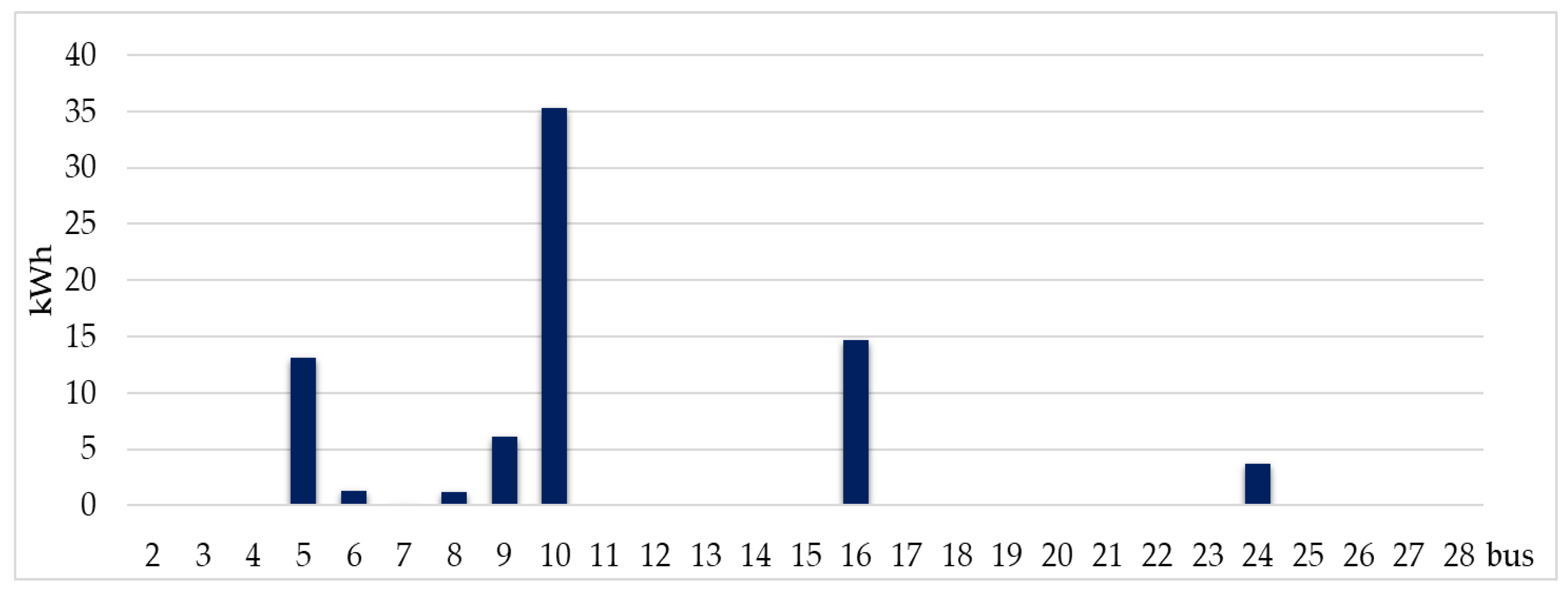
Scn3	0.000	0.000	0.000	13.134	1.310	0.116	1.141	6.088	35.305
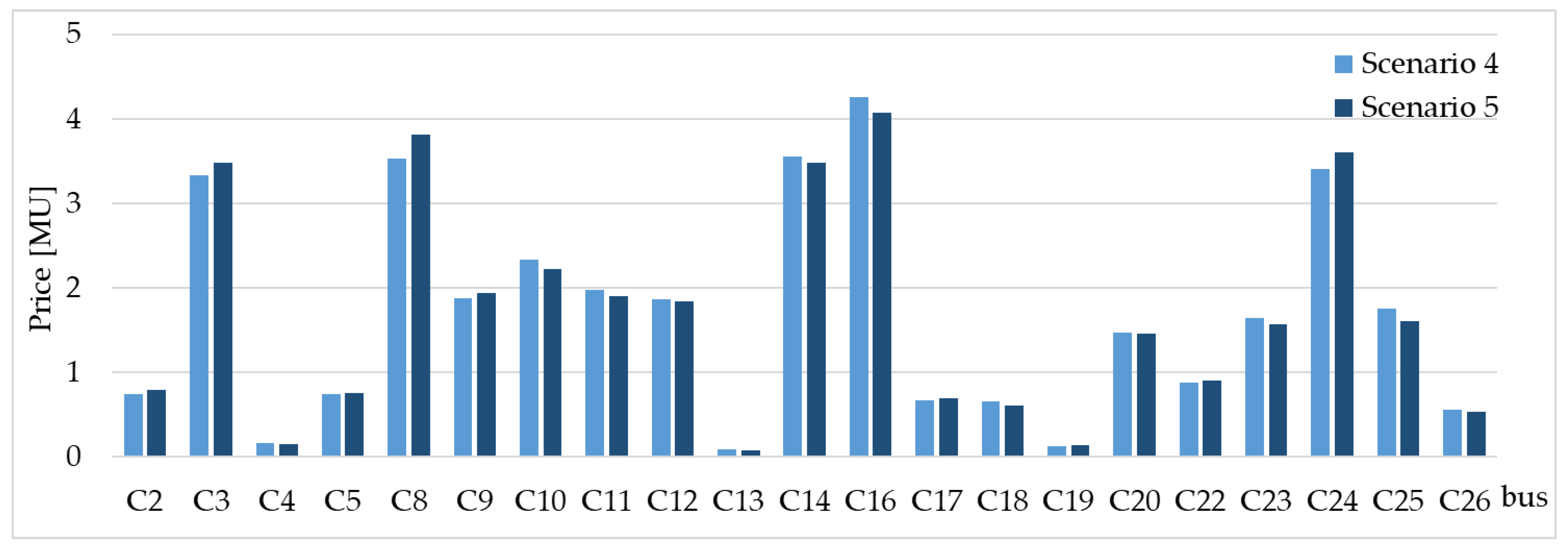
Scn4	1.678	7.109	0.378	1.489	0.000	0.000	7.430	3.927	5.133
Scn5	1.678	7.109	0.378	1.489	0.000	0.000	7.430	3.927	5.133
Scn./Cons.	C11	C12	C13	C14	C15	C16	C17	C18	C19
Scn1	1.615	2.036	2.546	17.973	0.000	0.000	0.000	0.000	0.963
Scn2	2.232	0.000	0.000	0.000	0.000	6.964	0.000	0.000	0.000
Scn3	0.000	0.000	0.000	0.000	0.000	14.654	0.000	0.000	0.000
Scn4	4.340	3.885	0.206	7.460	0.000	8.814	1.625	1.407	0.315
Scn5	4.340	3.885	0.206	7.460	0.000	8.814	1.625	1.407	0.315
Scn./Cons.	C20	C21	C22	C23	C24	C25	C26	C27	C28
Scn1	9.949	0.000	3.597	3.654	0.740	6.919	4.191	0.000	0.265
Scn2	1.805	0.000	0.000	0.000	6.882	0.000	1.980	0.000	0.000
Scn3	0.000	0.000	0.000	0.000	3.733	0.000	0.000	0.000	0.000
Scn4	2.822	0.000	1.901	3.500	7.187	3.612	1.264	0.000	0.001
Scn5	2.822	0.000	1.901	3.500	7.187	3.612	1.264	0.000	0.001

. For the first scenario (Scn₁), the quantities traded by prosumers to consumers are shown in Figure 6. It can be seen that the consumers geographically close from prosumers locations purchase the higher quantities. For example, the prosumer P7 sells energy to consumer C8, prosumer P15 to consumer C14, and the prosumer P21 to consumer C20. Similar results are obtained for Scenario 2 (Scn₂) where the prioritization is made according to the instantaneous power required by consumers. In this scenario, the consumers with the highest demand are preferred in the same manner, in each trading interval (C10, C9, C8, C5), as seen in Figure 6 and Table 5.

For Scenario 3, where consumers are allocated in five priority clusters according to the daily electricity demand (Figure 5), it is observed that cluster I already contains three prosumers (P6, P7 and P15) and one consumer (C10). Cluster II has a prosumer (P21) and two consumers (C5 and C16), and cluster III comprises of eight peers, and the last two clusters group the rest of the peers.

From Figure 7, it can be observed that the peers from the first two clusters have priority for trading, and the remaining surplus is sold only three consumers from cluster III, respectively C8, C9 and C24. In this scenario, the prosumer from bus 6 receives electricity from the local market, in the hours with deficit (see Table 2).

In the last two scenarios, that use the blockchain technology based on the FCFS principle, depending on the P2P contracts already signed, it is observed that the only ones who do not receive the surplus of electricity are prosumers an the consumer from bus 28, which has an insignificant consumption (see Table A1, Appendix A).

Figure 8 shows the similarities in traded quantities, resulting from applying the mathematical model proposed for the last two scenarios. The differences between Scn₄ and Scn₅ are seen in the purchase price of the surplus according to the type of P2P contract concluded between prosumers and the rest of the participants in the network.

For all five scenarios, the daily electricity quantities from prosumers purchased by consumers are presented in

Table 6. The prosumers energy surplus trading (kWh) and prices (MU/kWh) in Scenario 1.

Bus	The Active Energy Surplus					Total kWh	P2P Price	Total Cost/Revenue
	P6	P7	P15	P21	P27			for Cj	for Pk
2	0.000	0.000	0.000	0.000	0.136	0.136	0.058	0.098	0.030
5	8.532	0.000	0.000	0.000	0.000	8.532	3.669	6.143	1.903
8	2.366	9.921	0.000	0.000	0.000	12.287	4.986	8.847	2.740
9	0.000	0.077	0.000	0.000	0.000	0.077	0.031	0.055	0.017
11	0.000	0.000	1.615	0.000	0.000	1.615	0.775	1.163	0.360
12	0.000	0.000	2.036	0.000	0.000	2.036	0.977	1.466	0.454
13	0.000	0.000	2.546	0.000	0.000	2.546	1.222	1.833	0.568
14	0.000	0.000	17.973	0.000	0.000	17.973	8.627	12.941	4.008
19	0.000	0.000	0.000	0.963	0.000	0.963	0.529	0.693	0.215
20	0.000	0.000	0.000	9.949	0.000	9.949	5.472	7.164	2.219
22	0.000	0.000	0.000	3.597	0.000	3.597	1.979	2.590	0.802
23	0.000	0.000	0.000	3.654	0.000	3.654	2.010	2.631	0.815
24	0.000	0.000	0.000	0.740	0.000	0.740	0.407	0.533	0.165
25	0.000	0.000	0.000	0.000	6.919	6.919	2.975	4.982	1.543
26	0.000	0.000	0.000	0.000	4.191	4.191	1.802	3.018	0.935
28	0.000	0.000	0.000	0.000	0.265	0.265	0.114	0.191	0.059

,

Table 7. The prosumers energy surplus trading (kWh) and prices (MU/kWh) in Scenario 2.

Bus	The Active Energy Surplus, in kWh					Total kWh	P2P Price	Total Cost/Revenue
	P6	P7	P15	P21	P27			for Cj	for Pk
3	0.000	0.000	0.000	1.588	0.000	1.588	0.873	1.143	0.354
5	2.295	2.105	1.957	0.000	1.595	7.951	3.454	5.725	1.773
8	0.000	0.000	5.088	3.693	0.000	8.781	4.473	6.322	1.958
9	0.000	1.356	7.315	3.859	3.443	15.973	7.657	11.501	3.562
10	7.488	4.256	4.406	1.867	3.308	21.325	9.486	15.354	4.755
11	0.000	0.000	1.062	1.170	0.000	2.232	1.153	1.607	0.498
16	0.000	2.281	1.302	1.726	1.655	6.964	3.198	5.014	1.553
20	0.000	0.000	0.000	1.805	0.000	1.805	0.993	1.300	0.403
24	1.116	0.000	1.880	2.376	1.510	6.882	3.339	4.955	1.535
26	0.000	0.000	1.161	0.819	0.000	1.980	1.008	1.425	0.441

,

Table 8. The prosumers energy surplus trading (kWh) and prices (MU/kWh) in Scenario 3.

Bus	The Active Energy Surplus, in kWh					Total kWh	P2P Price	Total Cost/Revenue
	P6	P7	P15	P21	P27			for Cj	for Pk
5	0.000	0.058	5.091	5.604	2.381	13.134	6.573	9.456	2.929
6	0.000	0.000	0.208	1.102	0.000	1.310	0.706	0.943	0.292
7	0.000	0.000	0.116	0.000	0.000	0.116	0.056	0.084	0.026
8	0.000	0.000	0.000	0.000	1.141	1.141	0.491	0.822	0.255
9	0.000	0.000	0.012	3.301	2.775	6.088	3.014	4.383	1.358
10	10.899	8.954	12.399	2.491	0.563	35.305	15.831	25.420	7.873
16	0.000	0.986	6.345	4.595	2.728	14.654	7.140	10.551	3.268
24	0.000	0.000	0.000	1.811	1.922	3.733	1.822	2.688	0.832

,

Table 9. The prosumers energy surplus trading (kWh) and prices (MU/kWh) in Scenario 4.

Bus	The Active Energy Surplus, in kWh					Total kWh	P2P Price	Total Cost/Revenue
	P6	P7	P15	P21	P27			for Cj	for Pk
2	0.860	0.000	0.000	0.176	0.641	1.678	0.743	1.208	0.374
3	0.000	1.154	2.962	1.394	1.599	7.109	3.338	5.118	1.585
4	0.378	0.000	0.000	0.000	0.000	0.378	0.163	0.272	0.084
5	0.000	0.000	0.181	0.749	0.559	1.489	0.739	1.072	0.332
8	0.244	1.048	0.603	2.761	2.773	7.430	3.525	5.350	1.657
9	0.000	0.002	2.046	0.773	1.106	3.927	1.884	2.827	0.876
10	2.295	1.356	0.122	1.361	0.000	5.133	2.336	3.695	1.145
11	1.845	0.745	1.130	0.620	0.000	4.340	1.975	3.125	0.968
12	0.000	0.645	2.572	0.668	0.000	3.885	1.860	2.797	0.866
13	0.150	0.056	0.000	0.000	0.000	0.206	0.087	0.148	0.046
14	1.116	0.691	2.141	2.140	1.372	7.460	3.551	5.371	1.664
16	1.917	1.632	1.634	3.631	0.000	8.814	4.259	6.346	1.966
17	0.000	1.331	0.294	0.000	0.000	1.625	0.674	1.170	0.362
18	0.000	0.263	1.144	0.000	0.000	1.407	0.654	1.013	0.314
19	0.000	0.298	0.017	0.000	0.000	0.315	0.127	0.227	0.070
20	0.000	0.000	1.100	1.722	0.000	2.822	1.475	2.032	0.629
22	0.412	0.000	1.136	0.000	0.353	1.901	0.874	1.369	0.424
23	0.000	0.410	3.090	0.000	0.000	3.500	1.647	2.520	0.781
24	0.000	0.000	2.430	1.649	3.108	7.187	3.410	5.174	1.603
25	0.742	0.368	1.242	1.260	0.000	3.612	1.755	2.601	0.805
26	0.940	0.000	0.324	0.000	0.000	1.264	0.560	0.910	0.282

and

Table 10. The prosumers energy surplus trading (kWh) and prices (MU/kWh) in Scenario 5.

Bus	The Active Energy Surplus, in kWh					Total kWh	P2P Price	Total Cost/Revenue
	P6	P7	P15	P21	P27			for Cj	for Pk
2	0.000	0.860	0.000	0.817	0.000	1.678	0.794	1.208	0.374
3	0.889	0.000	2.610	2.430	1.179	7.109	3.479	5.118	1.585
4	0.000	0.378	0.000	0.000	0.000	0.378	0.151	0.272	0.084
5	0.000	0.000	0.930	0.559	0.000	1.489	0.754	1.072	0.332
8	1.184	0.108	0.546	4.988	0.603	7.430	3.818	5.350	1.657
9	0.002	0.000	0.538	1.879	1.508	3.927	1.941	2.827	0.876
10	2.663	1.413	1.056	0.000	0.000	5.133	2.217	3.695	1.145
11	1.690	1.397	0.000	0.620	0.633	4.340	1.899	3.125	0.968
12	0.000	0.000	3.153	0.087	0.645	3.885	1.839	2.797	0.866
13	0.056	0.150	0.000	0.000	0.000	0.206	0.084	0.148	0.046
14	0.047	1.093	2.906	1.331	2.083	7.460	3.480	5.371	1.664
16	2.031	1.517	3.289	1.308	0.668	8.814	4.066	6.346	1.966
17	0.886	0.000	0.000	0.000	0.739	1.625	0.699	1.170	0.362
18	0.000	0.263	0.214	0.000	0.930	1.407	0.608	1.013	0.314
19	0.298	0.000	0.000	0.000	0.017	0.315	0.135	0.227	0.070
20	0.000	0.000	1.410	1.412	0.000	2.822	1.453	2.032	0.629
22	0.000	0.412	1.136	0.353	0.000	1.901	0.904	1.369	0.424
23	0.000	0.410	1.477	0.000	1.613	3.500	1.567	2.520	0.781
24	1.152	0.000	3.031	3.003	0.000	7.187	3.602	5.174	1.603
25	0.000	1.056	1.547	0.117	0.892	3.612	1.613	2.601	0.805
26	0.000	0.940	0.324	0.000	0.000	1.264	0.532	0.910	0.282

. Moreover, the last four columns from the aforementioned tables contain the total quantities purchased by each consumer, the price paid by consumer(s) to prosumers for this quantity trough P2P contracts, the regulated price that should have been paid by consumers to the classical supplier at 0.72 MU/kWh, and also by prosumers to the grid aggregator with a regulated price of 0.223 MU/kWh. The last columns present the financial advantages for all the transaction participants.

To highlight the prosumer/consumer advantages using the proposed PEST algorithm, from Table 6, Table 7, Table 8, Table 9 and Table 10 can be seen the benefits registered by each participant in the trading process, regardless of the chosen prioritization scenario.

For example, in Figure 9 the prosumers financial benefits were presented, with the price paid for the consumers to each prosumer trough the smart considered P2P contracts compared to the regulated price received if they injected the surplus directly into the μG.

The benefits of using the local market are also present for the consumers. In Figure 10, the differences between the regulated price that would be paid by consumers and the P2P price used in trading with the prosumers are presented, which is always lower. For the equal quantities traded in Scenarios 4 and 5, the differences in financial settlements resulting from the blockchain merit order, but with different prosumer-consumer trading prices are presented in Figure 11.

5. Discussion

As the results presented in the study case show, both the consumers and the prosumers can obtain significant profits from the implementation of a local μM in which prosumers sell directly to the prosumers. In this market, prosumer can sell electricity to prosumers at prices lower than the regulated tariff established for residential consumers, but higher than the price at which they can sell back to the grid their generation surplus. As in Figure 9, the daily profits for prosumers can vary from 1.8 to 6.2 MU (1 MU = 1 Romanian leu or 0.21 EUR), and for consumers from 1.8 to 6.2 MU.

For consumers, the daily financial gain can amount to up to 2.2 MU (consumer C16). The consumer’s total demand for the considered day is of 23.84 kWh, amounting to an electricity bill of 17.16 MU, which means that the daily saving of the consumer is of 12.8%, in the scenario with the maximum number of consumers involved in trading. Our proposed mechanism was tested also for the cases when the PV generation of the prosumers is small. In these cases, if it is a surplus, the most convenient turned out to be Scenario 4 based on the blockchain technologies, which consider both quantities and price (from P2P contracts).

For a technical consideration, it should be noted that the trading results presented in the paper do not account for the energy losses in the LV distribution network, because they have the same influence on all the scenarios considered in the algorithm. In the physical network, prosumers would inject the surplus in the local network, and the consumers would draw power in the same manner. The difference is only in the financial settlement performed in the μM. The losses need to be settled at the market level, but this is a separate mechanism that needs future research. In

Table 11. The prosumers energy surplus trading (kWh) and prices (MU/kWh).

No. of. Scenarios	No. of Consumers	Diff. of Common Consumers
Scn1	16	13
Scn2	10	7
Scn3	8	5
Scn4	21	18
Scn5	23	20

, the number of consumers which benefits form the trading process are presented. It can be seen that only three consumers are commonly to the five considered scenarios. For the three consumers in Figure 12, Figure 13 and Figure 14 the purchased energy and the costs of consumers, and the revenue of prosumers.

Considering the obtained results from Table 5, Table 6, Table 7, Table 8, Table 9 and Table 10 and Figure 7 and Figure 12, Figure 13 and Figure 14, it is emphasized that the third scenario is the least favorable for the participants. In this scenario, the distribution network operators win due to an optimization of power flows between the prosumers and the consumers with high power demand.

The time granularity and period of day was considered. Our study was conduct only hourly trading for a day, but the mechanism can be easily used for other period. A complete transaction depends upon the proposed scenarios, taking into account the surplus of the prosumers, consumers power demand, as well as the distance between peers and P2P contracts.

The proposed algorithm is only the first step in developing a trading platform for consumers and prosumers in microgrids, and is aimed to serve as a simulation tool for developing alternatives for the current regulation framework regarding prosumer activity in the Romanian electricity market. However, future research will extend its capabilities for other trading scenarios.

6. Patents

National Patent Application “Innovative method of decision-making assistance aimed at streamlining the management of prosumer activity”, Romania, 2019, in press.

References

- Huang, J.; Jiang, C.; Xu, R. A review on distributed energy resources and MicroGrid. Renew. Sustain. Energy Rev. 2008, 12, 2472–2483. [Google Scholar]
- Pudjianto, D.; Ramsay, C.; Strbac, G. Virtual power plant and system integration of distributed energy resources. IET Renew. Power Gener. 2007, 1, 10–16. [Google Scholar] [CrossRef]
- Hierzinger, R.; Albu, M.; van Elburg, H.; Scott, A.; Lazicki, A.; Penttinen, L.; Puente, F.; Saele, H. European Smart Metering Landscape Report 2012—Update May 2013; ÖSTERREICHISCHE ENERGIEAGENTUR–AUSTRIAN ENERGY AGENCY: Vienna, Austria, 2013. [Google Scholar]
- Kohlhepp, P.; Harb, H.; Wolisz, H.; Waczowicz, S.; Müller, D.; Hagenmeyer, V. Large-scale grid integration of residential thermal energy storages as demand-side flexibility resource: A review of international field studies. In Renewable and Sustainable Energy Reviews; Elsevier: Amsterdam, The Netherlands, 2019; Volume 101, pp. 527–547. [Google Scholar]
- Pitì, A.; Verticale, G.; Rottondi, C.; Capone, A.; Lo Schiavo, L. The role of smart meters in enabling real-time energy services for households: The Italian case. Energies 2017, 10, 199. [Google Scholar] [CrossRef]
- Mengelkamp, E.; Notheisen, B.; Beer, C.; Dauer, D.; Weinhardt, C. A blockchain-based smart grid: Towards sustainable local energy markets. Comput. Sci.-Res. Dev. 2018, 33, 207–214. [Google Scholar] [CrossRef]
- Zhang, C.; Wu, J.; Cheng, M.; Zhou, Y.; Long, C. A Bidding System for Peer-to-Peer Energy Trading in a Grid connected Microgrid. Energy Procedia 2016, 103, 147–152. [Google Scholar] [CrossRef]
- Espe, E.; Potdar, V.; Chang, E. Prosumer Communities and Relationships in Smart Grids: A Literature Review, Evolution and Future Directions. Energies 2018, 11, 2528. [Google Scholar] [CrossRef]
- Andoni, M.; Robu, V.; Flynn, D.; Abram, S.; Geach, D.; Jenkins, D.; McCallum, P.; Peacock, A. Blockchain technology in the energy sector: A systematic review of challenges and opportunities. Renew. Sustain. Energy Rev. 2019, 100, 143–174. [Google Scholar] [CrossRef]
- Wu, J.; Tran, N. Application of blockchain technology in sustainable energy systems: An overview. Sustainability 2018, 10, 3067. [Google Scholar] [CrossRef]
- Kim, H.J.; Song, Y.H.; Kim, S.W.; Yoon, Y.T. Implementation of peer-to-peer energy auction based on transaction zoning considering network constraints. J. Int. Counc. Electr. Eng. 2019, 9, 53–60. [Google Scholar] [CrossRef]
- Liu, T.; Tan, X.; Sun, B.; Wu, Y.; Guan, X.; Tsang, D.H.K. Energy Management of Cooperative Microgrids with P2P Energy Sharing in Distribution Networks. In Proceedings of the IEEE International Conference on Smart Grid Communications (SmartGridComm), Miami, FL, USA, 2–5 November 2015; pp. 410–415. [Google Scholar]
- Di Silvestre, M.L.; Gallo, P.; Ippolito, M.G.; Musca, R.; Sanseverino, E.R.; Tran, Q.T.T.; Zizzo, G. Ancillary Services in the Energy Blockchain for Microgrids. IEEE Trans. Ind. Appl. 2019, 55, 7310–7319. [Google Scholar] [CrossRef]
- Wang, N.; Xu, W.; Xu, Z.; Shao, W. Peer-to-Peer Energy Trading among Microgrids with Multidimensional Willingness. Energies 2018, 11, 3312. [Google Scholar] [CrossRef]
- Kang, J.; Yu, R.; Huang, X.; Maharjan, S.; Zhang, Y.; Hossain, E. Enabling localized peer-to-peer electricity trading among plug-in hybrid electric vehicles using consortium blockchains. IEEE Trans. Ind. Inform. 2017, 13, 3154–3164. [Google Scholar] [CrossRef]
- Thakur, S.; Hayes, B.P.; Breslin, J.G. Distributed Double Auction for Peer to Peer Energy Trade Using Blockchains. In Proceedings of the 2018 5th International Symposium on Environment-Friendly Energies and Applications (EFEA), Rome, Italy, 24–26 September 2018; pp. 1–8. [Google Scholar]
- Khorasany, M.; Mishra, Y.; Ledwich, G. Design of auction-based approach for market clearing in peer-to-peer market platform. J. Eng. 2019, 2019, 4813–4818. [Google Scholar] [CrossRef]
- Islam, S.N. A New Pricing Scheme for Intra-Microgrid and Inter-Microgrid Local Energy Trading. Electronics 2019, 8, 898. [Google Scholar] [CrossRef]
- Leal-Arcas, R.; Lesniewska, F.; Proedrou, F. Prosumers as New Energy Actors. In Africa-EU Renewable Energy Research and Innovation Symposium; Springer: Berlin/Heidelberg, Germany, 2018; pp. 139–151. [Google Scholar]
- Zhang, C.; Wu, J.; Zhou, Y.; Cheng, M.; Long, C. Peer-to-Peer energy trading in a Microgrid. Appl. Energy 2018, 220, 1–12. [Google Scholar] [CrossRef]
- El Rahi, G.; Etesami, S.R.; Saad, W.; Mandayam, N.B.; Poor, H.V. Managing Price Uncertainty in Prosumer-Centric Energy Trading: A Prospect-Theoretic Stackelberg Game Approach. IEEE Trans. Smart Grid 2019, 10, 702–713. [Google Scholar] [CrossRef]
- Bremdal, B.A.; Olivella, P.; Rajasekharan, J. EMPOWER: A network market approach for local energy trade. In IEEE Manchester PowerTech; IEEE: Piscataway, NJ, USA, 2017; pp. 1–6. [Google Scholar]
- Cali, U.; Fifield, A. Towards the decentralized revolution in energy systems using blockchain technology. Int. J. Smart Grid Clean Energy 2019, 8, 245–256. [Google Scholar]
- Uslar, M.; Rohjans, S.; Neureiter, C.; Pröstl Andrén, F.; Velasquez, J.; Steinbrink, C.; Efthymiou, V.; Migliavacca, G.; Horsmanheimo, S.; Brunner, H.; et al. Applying the Smart Grid Architecture Model for Designing and Validating System-of-Systems in the Power and Energy Domain: A European Perspective. Energies 2019, 12, 258. [Google Scholar] [CrossRef]
- Jogunola, O.; Ikpehai, A.; Anoh, K.; Adebisi, B.; Hammoudeh, M.; Gacanin, H.; Harris, G. Comparative Analysis of P2P Architectures for Energy Trading and Sharing. Energies 2018, 11, 62. [Google Scholar] [CrossRef]
- Long, C.; Wu, J.; Zhang, C.; Cheng, M.; Al-Wakeel, A. Feasibility of peer-to-peer energy trading in low voltage electrical distribution networks. Energy Procedia 2017, 105, 2227–2232. [Google Scholar] [CrossRef]
- Yu, Q.; Meeuw, A.; Wortmann, F. Design and implementation of a blockchain multi-energy system. Energy Inform. 2018, 1, 17. [Google Scholar] [CrossRef]
- Paudel, A.; Chaudhari, K.; Long, C.; Gooi, H.B. Peer-to-Peer Energy Trading in a Prosumer-Based Community Microgrid: A Game-Theoretic Model. IEEE Trans. Ind. Electron. 2018, 66, 6087–6097. [Google Scholar] [CrossRef]
- Aldaouab, I.; Daniels, M.; Ordóñez, R. MPC for Optimized Energy Exchange between Two Renewable-Energy Prosumers. Appl. Sci. 2019, 9, 3709. [Google Scholar] [CrossRef]
- Hou, P.; Yang, G.; Hu, J.; Douglass, P.J.; Xue, Y. An Interactive Transactive Energy Mechanism Integrating Grid Operators, Aggregators and Prosumers. arXiv 2019, arXiv:1912.07139. [Google Scholar]
- Amanbek, Y.; Tabarak, Y.; Nunna, H.K.; Doolla, S. Decentralized Transactive Energy Management System for Distribution Systems with Prosumer Microgrids. In Proceedings of the 19th International Carpathian Control Conference (ICCC), Szilvasvarad, Hungary, 28–31 May 2018; pp. 553–558. [Google Scholar]
- Nizami, M.S.H.; Hossain, M.J.; Amin, B.M.R.; Kashif, M.; Fernandez, E.; Mahmud, K. Transactive Energy Trading of Residential Prosumers Using Battery Energy Storage Systems. In Proceedings of the 2019 IEEE Milan PowerTech, Milan, Italy, 23–27 June 2019; pp. 1–6. [Google Scholar]
- Le Cadre, H.; Jacquot, P.; Wan, C.; Alasseur, C. Peer-to-Peer Electricity Market Analysis: From Variational to Generalized Nash Equilibrium. Eur. J. Oper. Res. 2020, 282, 753–771. [Google Scholar] [CrossRef]
- Neagu, B.C.; Grigoras, G.; Ivanov, O. An Efficient Peer-to-Peer Based Blokchain Approach for Prosumers Energy Trading in Microgrids. In Proceedings of the International Conference on Modern Power Systems (MPS), Cluj Napoca, Romania, 21–23 May 2019; pp. 1–4. [Google Scholar]
- Barrero-González, F.; Pires, V.F.; Sousa, J.L.; Martins, J.F.; Milanés-Montero, M.I.; González-Romera, E.; Romero-Cadaval, E. Photovoltaic Power Converter Management in Unbalanced Low Voltage Networks with Ancillary Services Support. Energies 2019, 12, 972. [Google Scholar] [CrossRef]
- All You Need to Know to Become a prosumer. Available online: https://energyindustryreview.com/renewables/all-you-need-to-know-to-become-a-prosumer/ (accessed on 18 December 2019).
- National Regulatory Authority for Energy. The 228 Order for the Approval of the Technical Norm Technical Conditions for Connection to the Public Electrical Networks of the Prosumers; National Regulatory Authority for Energy: Bucharest, Romania, 2018.