Optimal Phase Load Balancing in Low Voltage Distribution Networks Using a Smart Meter Data-Based Algorithm

 ,
,  ,
, 

Abstract

1. Introduction
- Constructive imbalances. These appear because of the spatial arrangement of the phase conductors, at the electrical lines, and the arrangement of the windings on the three columns of the ferromagnetic core, at the power transformers.
- Functional imbalances. These are created by 1-P consumers. They are connected between two phases or between a phase and the neutral point. Many of them are represented by domestic and tertiary consumers supplied from the low-voltage (LV) network, with small values of the absorbed power (up to 100 kVA). Also, there are 1-P industrial consumers. They have high absorbed powers being connected to electric medium voltage (MV) networks. The representative 1-P industrial consumers are the following: the welding installations, with absorbed powers between 100 kVA and 3 MVA, the 1-P arc furnaces, and the electric stations that supply power the railway traction network).
- It can be implemented in the EDNs with hybrid structures of the consumption points (switchable and non-switchable 1-P consumers). The three-phase (3-P) consumers, having identical loadings on the three phases, are not considered in the algorithm, belonging to the non-switchable consumers’ category.
- It can work in both operation modes (real-time and off-line), uploading information from different databases of the DNO. The consumers’ characteristics (connecting pillar, allocated phase, consumption sector and class, integration in the SMS, identification number of the meter) are extracted based on the identification number of the supply point. The value of consumption and operating status of phase load balancing device (PLBD) are uploaded from the database of the SMS if the meter is integrated, or from the typical load profiles (TLPs) database if the consumer has a standard energy meter (non-integrated in the SMS).
- The convergence is rapid because of the fast recognition of the EDN topology with the help of a structure vectors-based algorithm. The optimal solutions for PLB are found at the level of each pillar such that the global solution obtained for the level of the supply point will be also optimal.
2. The Proposed PLB Algorithm
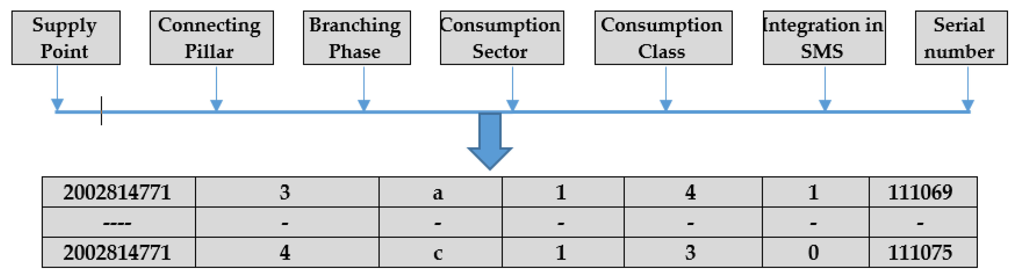
- Supply point: Each electric distribution substation has an identification number that allows the algorithm to allocate correct data from the database to all consumers supplied from this point.
- Connecting pillar: The connecting pillar is recorded in the database to identify the position of each consumer in the network. Also, this information is very important in the calculus of a steady-state regime to evaluate the performance of the PLB measure through reducing the power/energy losses and improving the voltage level at the consumers. The vector associated with this field is noted with CP, having the size (NC × 1), where NC represents the total number of consumers from the EDN.
- Branching Phase: Each 1-P consumer is allocated by the DNO at one of the phases ph = {a, b, c}, and the 3-P consumers are connected at all three phases ph = {a, b, c}. The records regarding this information are found in the vector PB with the size (NC × 1).
- Consumption Sector. The information is used to assign the consumer to the following consumption sectors: domestic, non-domestic, commercial, and industrial. The records for this information have the identification numbers from 1 to 4: 1 (domestic), 2 (non-domestic), 3 (commercial), and 4 (industrial) included in the vector CS with the size (NC × 1).
- Consumption class. More consumption classes are allocated to each consumption sector by the DNO. As an example, a Romanian DNO has a classification in five consumption classes for consumers from the domestic sector [36]: < 400 kWh (first class), range [400 kWh, 1250 kWh] (second class), range [1250 kWh, 2500 kWh] (third class), range [2500 kWh, 3500 kWh] (the fourth class), and range [2500 kWh, 3500 kWh] (the fifth class). This information is loaded in the vector CC, having the size (NC × 1).
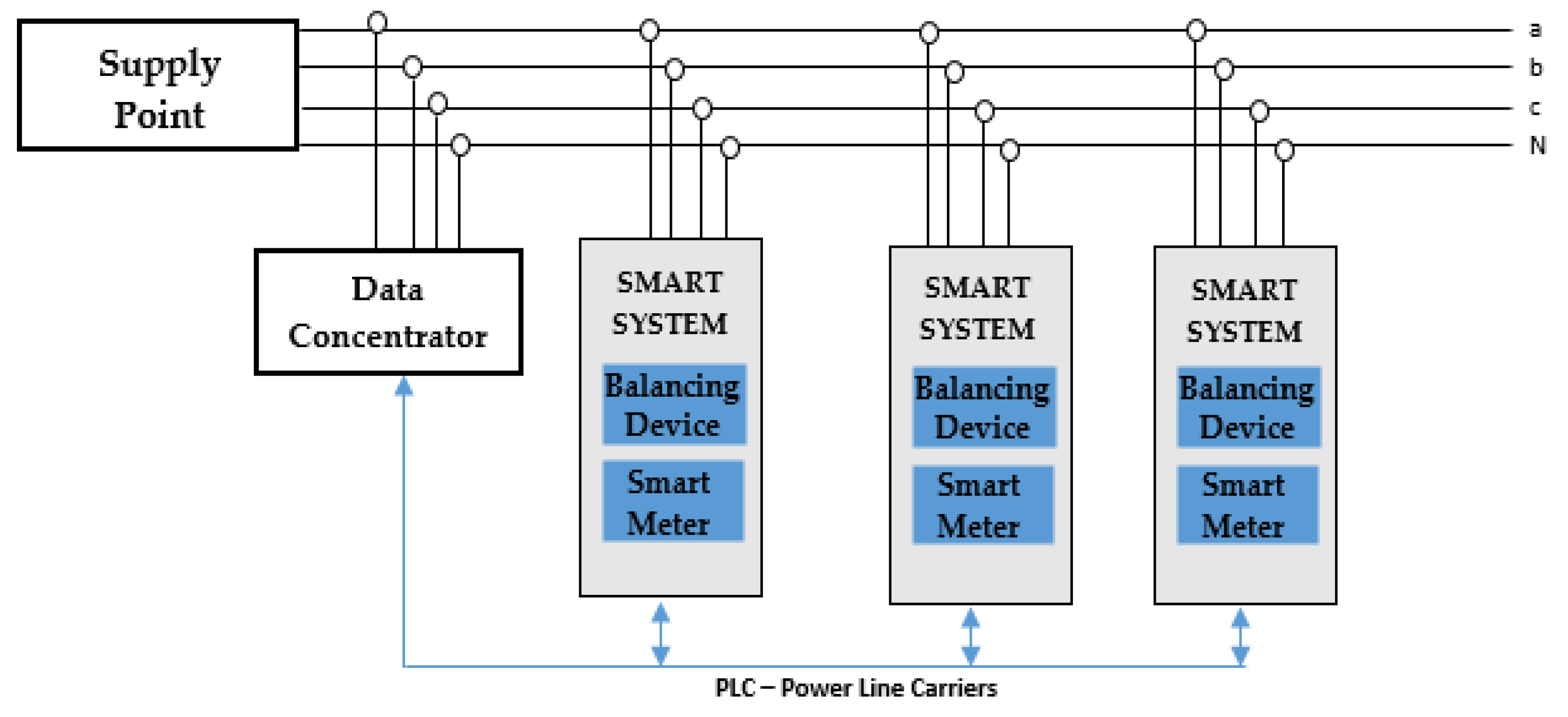
- Integration in SMS. Currently, not all consumers from the LV distribution networks are integrated into the smart metering system. In this case, the value 1 (if it is integrated) and 0 (otherwise) will be recorded in the database. If the meter is integrated into the SMS, it can communicate to the central system information about the currents or active and reactive powers, which will record them in the database (see Figure 5).
- Serial number. Each consumer is recognized in the database through the serial number of meter installed (smart or standard). The information is recorded in the vector SN, having the size (NC × 1).
3. Case Study
4. Conclusions
Supplementary Materials
Author Contributions
Funding
Conflicts of Interest
Nomenclature
| 0 | Neutral conductor |
| 1-P | Single-phase consumer |
| 3-P | Three-phase consumer |
| EDN | Electric distribution network |
| LV | Low voltage |
| TLP | Typical load profile |
| DNO | Distribution network operator |
| SMS | Smart metering system |
| SMD | Smart meter data |
| PLB | Phase load balancing |
| PLC | Power-line communication |
| SCADA | Supervisory control and data acquisition |
| APLBD | Automatic phase load balancing device |
| SPLBS | Smart phase load balancing system |
| DMCL | Decision-making central level |
| PSO | Particle swarm optimization |
| AG | Genetic algorithm |
| MCLA | Minimum count of loads adjustment |
| H | The analyzed time period, [hours] |
| Bi | Vector of the input nodes of branches |
| Bj | Vector of the end nodes of branches |
| a, b, c | The phases of the EDN |
| abc | 3-P consumer in the input data files |
| {ph} | The set of phases {a, b, c} |
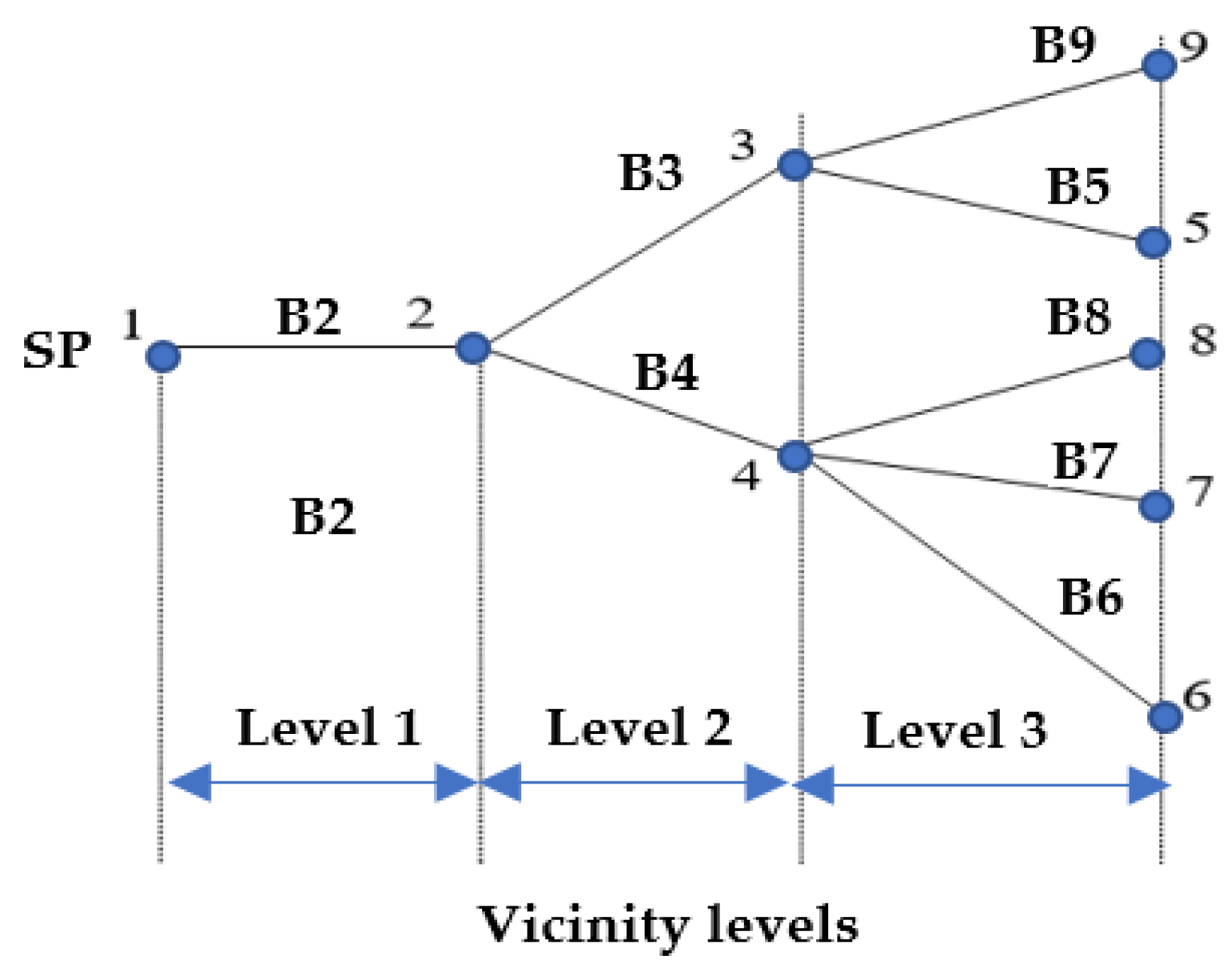
| TV1 | Topology vector containing the number of branches from each vicinity level |
| TV2 | Topology vector containing the branches placed in the order of the vicinity levels |
| SP | Supply Point |
| NC | The total number of consumers from the EDN |
| CP | Vector of the connected pillars, size (NC × 1) |
| PB | Vector of the branching phase, size (NC × 1) |
| CS | Vector of the consumption sector of the consumers, size (NC × 1) |
| CC | Vector of the consumption class of the consumers from a certain consumption sector, size (NC × 1) |
| INT | Vector of the integration mode in the SMS, size (NC × 1) |
| BS | Vector of the PLBD status, size (NC × 1) |
| IC | Vector of the hourly loads for all consumers, size (NC × H) |
| SN | Vector of the serial numbers corresponding the smart meters, size (NC × 1) |
| r0 | Specific resistance, [Ω/km] |
| x0 | Specific reactance, [Ω/km] |
| UC | The unbalance coefficient |
| Ia, Ib, Ic | The currents on the phases a, b, and c, [A] |
| Iaverage | The average value of the phase currents, [A] |
| h | The current hour (h = 1, …, H) |
| Np | The number of pillars from the EDN |
| p | The analyzed current pillar (p = 1, …, Np) |
| d | Pillar located downstream by pillar p |
| UC(p),h | The unbalance coefficient calculated at the pillar p and hour h |
| index | Vector of the indices corresponding to pillar p in vector CP |
| Ia(p),h | The current on the phase a, at the pillar p and hour h, [A] The current on the phase b, at the pillar p and hour h, [A] |
| Ic(p),h | The current on the phase c, at the pillar p and hour h, [A] |
| Ia,ns(p),h | The total current of the non-switchable consumers on the phase a, pillar p and hour h, [A] |
| Ib,ns(p),h | The total current of the non-switchable consumers on the phase b, pillar p and hour h, [A] |
| Ic,ns(p),h | The total current of the non-switchable consumers on the phase c, pillar p and hour h, [A] |
| Ia,s(p),h | The total current of the switchable consumers on the phase a, pillar p and hour h, [A] |
| Ib,s(p),h | The total current of the switchable consumers on the phase b, pillar p and hour h, [A] |
| Ic,s(p),h | The total current of the switchable consumers on the phase c, pillar p and hour h, [A] |
| Ia(d),h | The currents on the phase a, pillar d, and hour h, [A] |
| Ib,s(d),h | The currents on the phase b, pillar d, and hour h, [A] |
| Ic,s(d),h | The currents on the phase c, pillar d, and hour h, [A] |
| j | Index of the non-switchable consumer connected on the phase a, pillar p, and hour h |
| k | Index of the non-switchable consumer connected on the phase b, pillar p, and hour h |
| l | Index of the non-switchable consumer connected on the phase c, pillar p, and hour h |
| m | Index of the switchable consumer connected on the phase a, pillar p, and hour h |
| n | Index of the switchable consumer connected on the phase b, pillar p, and hour h |
| o | Index of the switchable consumer connected on the phase c, pillar p, and hour h |
| Na,ns(p),h | The number of the non-switchable consumers connected on the phase a, pillar p, and hour h |
| Nb,ns(p),h | The number of the non-switchable consumers connected on the phase b, pillar p, and hour h |
| Nc,ns(p),h | The number of the non-switchable consumers connected on the phase c, pillar p, and hour h |
| Na,s(p),h | The number of the switchable consumers connected on the phase a, pillar p, and hour h |
| Nb,s(p),h | The number of the switchable consumers connected on the phase b, pillar p, and hour h |
| Nc,s(p),h | The number of the switchable consumers connected on the phases c, pillar p, and hour h |
| NC,ns(p),h | The total number of the non-switchable consumers connected at the pillar p, and hour h |
| NC,s(p),h | The total number of the switchable consumers connected at the pillar p, and hour h |
| NC(p),h | The total number of the consumers connected at the pillar p, and hour h |
| Ia,ns,j(p),h | The current of the non-switchable consumer j (j = 1,…, Na,ns(p),h), [A] |
| Ib,ns,k(p),h | The current of the non-switchable consumer k (k = 1, …, Nb,ns(p),h), [A] |
| Ic,ns,l(p),h | The current of the non-switchable consumer l (l = 1, …, Nc,ns(p),h), [A] |
| Ia,s,m(p),h | The current of the switchable consumer m (m = 1, …, Na,s(p),h), [A] |
| Ia,s,n(p),h | The current of the switchable consumer n (n = 1, …, Nb,s(p),h), [A] |
| Ia,s,o(p),h | The current of the switchable consumer o (o = 1, …, Nc,s(p),h), [A] |
| δΔW | The percentage error, [%] |
Appendix A

| Pillar | Consumer’ Type | Branching Phase | Consumption Sector | Pillar | Consumer’ Type | Branching Phase | Consumption Sector | ||||||||||
|---|---|---|---|---|---|---|---|---|---|---|---|---|---|---|---|---|---|
| 1-P | 3-P | a | b | c | 1 | 2 | 3 | 1-P | 3-P | a | b | c | 1 | 2 | 3 | ||
| 8 | 2 | - | - | 2 | - | 1 | - | - | 51 | 2 | - | - | 1 | 1 | 1 | - | - |
| 9 | 2 | - | - | 2 | - | 1 | - | - | 52 | 3 | - | - | 3 | - | 1 | - | - |
| 10 | 3 | - | 2 | 1 | - | 1 | - | - | 53 | 1 | - | - | 1 | - | - | 2 | - |
| 11 | 1 | - | - | 1 | - | 1 | - | - | 54 | 6 | - | - | - | 6 | 1 | - | - |
| 12 | 2 | - | - | 2 | - | 1 | - | - | 55 | 2 | - | 1 | 1 | - | 1 | - | - |
| 13 | 1 | - | - | 1 | - | 1 | - | - | 56 | 2 | - | - | 2 | - | 1 | - | - |
| 14 | 2 | - | - | - | 2 | 1 | - | - | 57 | 1 | - | - | 1 | - | 1 | - | - |
| 15 | 2 | - | - | 1 | 1 | 1 | - | - | 58 | 1 | - | 1 | - | - | 1 | - | - |
| 17 | 1 | 1 | 1 | 1 | 1 | 1 | - | - | 59 | 2 | - | - | 2 | - | 1 | - | - |
| 18 | 2 | - | - | - | 2 | 1 | - | - | 60 | 2 | - | 1 | 1 | - | 1 | - | - |
| 19 | 2 | - | 2 | - | - | 1 | - | - | 61 | 1 | - | - | 1 | - | 1 | - | - |
| 20 | 2 | - | 2 | - | - | 1 | - | - | 62 | 1 | - | - | - | 1 | 1 | - | - |
| 21 | 1 | - | 1 | - | - | 1 | - | - | 63 | 2 | - | 2 | - | - | 1 | - | - |
| 22 | 2 | - | 1 | 1 | - | 1 | - | - | 65 | 1 | - | - | 1 | - | 1 | - | - |
| 23 | 2 | - | 2 | - | - | 1 | - | - | 66 | 4 | - | 1 | 3 | - | 1 | - | - |
| 24 | 1 | - | - | - | 1 | 1 | - | - | 67 | 2 | - | - | 2 | - | 1 | - | - |
| 26 | 2 | - | - | - | 2 | 1 | - | - | 68 | 2 | - | - | 2 | - | 1 | - | - |
| 27 | 3 | - | 1 | - | 2 | 1 | - | - | 69 | 2 | - | 1 | 1 | - | 1 | - | - |
| 28 | 2 | - | - | 1 | 1 | 1 | - | - | 70 | 1 | - | - | 1 | - | 1 | - | - |
| 29 | 4 | - | - | 1 | 3 | 1 | - | - | 71 | 1 | - | - | 1 | - | 1 | - | - |
| 30 | 2 | - | - | - | 2 | 1 | - | - | 72 | 1 | - | - | 1 | - | 1 | - | - |
| 31 | 2 | - | - | - | 2 | 1 | - | - | 75 | 2 | - | - | 2 | - | 1 | - | - |
| 32 | 1 | - | - | - | 1 | 1 | - | - | 76 | 2 | - | - | 2 | - | 1 | - | - |
| 33 | 4 | - | - | - | 4 | 1 | - | - | 77 | 2 | - | 1 | 1 | - | 1 | - | - |
| 34 | 5 | - | - | - | 5 | 1 | - | - | 78 | 4 | - | 1 | 3 | - | 1 | - | - |
| 35 | 4 | - | 1 | 1 | 2 | 1 | - | - | 79 | 1 | 1 | 1 | 2 | 1 | 1 | - | - |
| 36 | 1 | - | - | 1 | - | 1 | - | - | 80 | 2 | - | 2 | - | 1 | - | - | |
| 37 | 3 | - | - | - | 3 | 1 | - | - | 82 | 2 | - | - | 2 | - | 1 | - | - |
| 38 | 1 | - | - | - | 1 | 1 | - | - | 83 | 1 | - | 1 | - | - | 1 | - | - |
| 39 | 4 | - | - | 1 | 3 | 1 | - | - | 84 | 2 | - | - | 2 | - | 1 | - | - |
| 40 | 3 | - | - | - | 3 | 1 | - | - | 86 | 1 | - | - | 1 | - | 1 | - | - |
| 41 | 1 | - | - | - | 1 | 1 | - | - | 87 | 2 | - | - | 2 | - | 1 | - | - |
| 42 | 1 | - | - | - | 1 | 1 | - | - | 88 | 1 | - | - | 1 | - | 1 | - | - |
| 43 | 2 | - | - | - | 2 | 1 | - | - | 89 | 2 | - | - | 2 | - | 1 | - | - |
| 44 | 2 | - | - | 1 | 1 | 1 | - | - | 90 | 1 | - | - | 1 | - | 1 | - | - |
| 45 | 4 | - | - | - | 4 | 1 | - | - | 91 | 2 | - | - | 2 | - | 1 | - | - |
| 46 | 2 | - | - | - | 2 | 1 | - | - | 92 | 1 | - | - | 1 | - | 1 | - | - |
| 47 | 3 | - | 1 | 2 | - | 1 | - | - | 93 | 2 | - | - | 2 | - | 1 | - | - |
| 48 | 3 | - | 1 | 2 | - | 1 | 2 | - | 94 | 1 | - | 1 | - | - | 1 | - | - |
| 49 | 2 | - | - | 2 | - | 1 | - | - | 95 | 1 | - | - | 1 | - | 1 | - | - |
| 50 | 1 | - | - | - | 1 | 1 | - | - | |||||||||
Appendix B
| Hour | Without | SMD (Proposed) | MCLA | PSO | GA |
|---|---|---|---|---|---|
| 1 | 1.2949 | 1.0000 | 1.0001 | 1.0017 | 1.0010 |
| 2 | 1.2965 | 1.0000 | 1.0005 | 1.0023 | 1.0009 |
| 3 | 1.2923 | 1.0000 | 1.0007 | 1.0024 | 1.0007 |
| 4 | 1.3016 | 1.0000 | 1.0012 | 1.0026 | 1.0011 |
| 5 | 1.2837 | 1.0000 | 1.0010 | 1.0029 | 1.0007 |
| 6 | 1.2265 | 1.0006 | 1.0005 | 1.0023 | 1.0003 |
| 7 | 1.1840 | 1.0042 | 1.0017 | 1.0010 | 1.0027 |
| 8 | 1.1700 | 1.0070 | 1.0042 | 1.0021 | 1.0046 |
| 9 | 1.2036 | 1.0050 | 1.0040 | 1.0004 | 1.0017 |
| 10 | 1.2630 | 1.0003 | 1.0022 | 1.0007 | 1.0000 |
| 11 | 1.3041 | 1.0000 | 1.0039 | 1.0018 | 1.0007 |
| 12 | 1.3339 | 1.0002 | 1.0031 | 1.0029 | 1.0019 |
| 13 | 1.3485 | 1.0003 | 1.0026 | 1.0040 | 1.0028 |
| 14 | 1.3209 | 1.0001 | 1.0028 | 1.0028 | 1.0016 |
| 15 | 1.3313 | 1.0001 | 1.0027 | 1.0031 | 1.0023 |
| 16 | 1.3078 | 1.0001 | 1.0012 | 1.0030 | 1.0013 |
| 17 | 1.3198 | 1.0001 | 1.0025 | 1.0030 | 1.0021 |
| 18 | 1.2881 | 1.0001 | 1.0018 | 1.0010 | 1.0006 |
| 19 | 1.2344 | 1.0025 | 1.0011 | 1.0001 | 1.0003 |
| 20 | 1.1843 | 1.0049 | 1.0029 | 1.0025 | 1.0032 |
| 21 | 1.1691 | 1.0070 | 1.0040 | 1.0053 | 1.0058 |
| 22 | 1.1867 | 1.0051 | 1.0031 | 1.0028 | 1.0032 |
| 23 | 1.2241 | 1.0024 | 1.0021 | 1.0007 | 1.0008 |
| 24 | 1.2562 | 1.0004 | 1.0005 | 1.0008 | 1.0001 |
| Hour | Without | SMD (Proposed) | MCLA | PSO | GA |
|---|---|---|---|---|---|
| 1 | 31.84 | 0.30 | 0.56 | 2.42 | 1.87 |
| 2 | 30.49 | 0.24 | 1.23 | 2.68 | 1.72 |
| 3 | 28.58 | 0.19 | 1.40 | 2.60 | 1.42 |
| 4 | 29.20 | 0.36 | 1.81 | 2.71 | 1.74 |
| 5 | 28.43 | 0.21 | 1.67 | 2.85 | 1.39 |
| 6 | 22.15 | 1.14 | 1.06 | 2.21 | 0.87 |
| 7 | 23.59 | 3.58 | 2.27 | 1.75 | 2.85 |
| 8 | 24.97 | 5.06 | 3.90 | 2.79 | 4.10 |
| 9 | 29.18 | 4.59 | 4.07 | 1.34 | 2.66 |
| 10 | 33.83 | 1.10 | 3.11 | 1.70 | 0.30 |
| 11 | 40.52 | 0.22 | 4.57 | 3.07 | 1.98 |
| 12 | 39.28 | 0.91 | 3.78 | 3.67 | 2.92 |
| 13 | 42.20 | 1.26 | 3.67 | 4.49 | 3.80 |
| 14 | 40.18 | 0.77 | 3.73 | 3.76 | 2.85 |
| 15 | 41.18 | 0.76 | 3.68 | 3.98 | 3.39 |
| 16 | 35.84 | 0.68 | 2.19 | 3.52 | 2.34 |
| 17 | 40.77 | 0.64 | 3.59 | 3.96 | 3.33 |
| 18 | 43.34 | 0.63 | 3.39 | 2.58 | 1.89 |
| 19 | 36.19 | 3.72 | 2.49 | 0.74 | 1.37 |
| 20 | 29.41 | 4.79 | 3.68 | 3.39 | 3.90 |
| 21 | 32.43 | 6.61 | 4.97 | 5.71 | 6.03 |
| 22 | 39.04 | 6.46 | 5.02 | 4.75 | 5.12 |
| 23 | 41.72 | 4.29 | 3.99 | 2.30 | 2.44 |
| 24 | 33.45 | 1.24 | 1.53 | 1.90 | 0.79 |
| Hour | SMD (Proposed) | MCLA | PSO | GA | ||||||||
|---|---|---|---|---|---|---|---|---|---|---|---|---|
| a | b | c | a | b | c | a | b | c | a | b | c | |
| 1 | 0.40 | 0.03 | 0.43 | 0.60 | 0.03 | 0.63 | 0.40 | 0.03 | 0.43 | 0.43 | 1.68 | 2.11 |
| 2 | 0.36 | 0.03 | 0.39 | 0.54 | 0.03 | 0.57 | 0.37 | 0.03 | 0.39 | 0.39 | 1.52 | 1.91 |
| 3 | 0.32 | 0.02 | 0.35 | 0.48 | 0.02 | 0.50 | 0.33 | 0.02 | 0.35 | 0.35 | 1.35 | 1.70 |
| 4 | 0.33 | 0.02 | 0.35 | 0.48 | 0.02 | 0.50 | 0.33 | 0.02 | 0.36 | 0.35 | 1.36 | 1.71 |
| 5 | 0.33 | 0.02 | 0.35 | 0.49 | 0.02 | 0.51 | 0.33 | 0.02 | 0.36 | 0.35 | 1.38 | 1.73 |
| 6 | 0.25 | 0.01 | 0.26 | 0.40 | 0.01 | 0.41 | 0.25 | 0.01 | 0.26 | 0.26 | 1.08 | 1.35 |
| 7 | 0.35 | 0.02 | 0.37 | 0.55 | 0.02 | 0.57 | 0.35 | 0.02 | 0.37 | 0.37 | 1.51 | 1.88 |
| 8 | 0.43 | 0.03 | 0.45 | 0.67 | 0.03 | 0.70 | 0.42 | 0.03 | 0.45 | 0.45 | 1.85 | 2.30 |
| 9 | 0.48 | 0.03 | 0.52 | 0.74 | 0.03 | 0.77 | 0.48 | 0.03 | 0.51 | 0.52 | 2.06 | 2.58 |
| 10 | 0.50 | 0.04 | 0.54 | 0.75 | 0.04 | 0.78 | 0.51 | 0.04 | 0.54 | 0.54 | 2.11 | 2.64 |
| 11 | 0.63 | 0.05 | 0.68 | 0.91 | 0.05 | 0.96 | 0.64 | 0.05 | 0.69 | 0.68 | 2.59 | 3.27 |
| 12 | 0.54 | 0.05 | 0.59 | 0.83 | 0.05 | 0.88 | 0.55 | 0.05 | 0.60 | 0.59 | 2.35 | 2.94 |
| 13 | 0.60 | 0.06 | 0.66 | 0.92 | 0.06 | 0.97 | 0.61 | 0.06 | 0.67 | 0.66 | 2.60 | 3.25 |
| 14 | 0.59 | 0.05 | 0.64 | 0.84 | 0.05 | 0.89 | 0.60 | 0.05 | 0.64 | 0.64 | 2.42 | 3.05 |
| 15 | 0.60 | 0.05 | 0.65 | 0.86 | 0.05 | 0.91 | 0.61 | 0.05 | 0.66 | 0.65 | 2.46 | 3.11 |
| 16 | 0.49 | 0.04 | 0.52 | 0.71 | 0.04 | 0.75 | 0.49 | 0.04 | 0.53 | 0.52 | 2.02 | 2.55 |
| 17 | 0.61 | 0.05 | 0.66 | 0.87 | 0.05 | 0.92 | 0.62 | 0.05 | 0.67 | 0.66 | 2.50 | 3.16 |
| 18 | 0.76 | 0.06 | 0.82 | 1.12 | 0.06 | 1.18 | 0.77 | 0.06 | 0.82 | 0.82 | 3.18 | 3.99 |
| 19 | 0.65 | 0.04 | 0.69 | 1.01 | 0.04 | 1.05 | 0.65 | 0.04 | 0.69 | 0.69 | 2.79 | 3.48 |
| 20 | 0.55 | 0.03 | 0.58 | 0.89 | 0.03 | 0.92 | 0.55 | 0.03 | 0.58 | 0.58 | 2.42 | 3.00 |
| 21 | 0.73 | 0.04 | 0.78 | 1.15 | 0.04 | 1.19 | 0.73 | 0.04 | 0.77 | 0.78 | 3.16 | 3.94 |
| 22 | 0.96 | 0.05 | 1.01 | 1.58 | 0.05 | 1.64 | 0.96 | 0.05 | 1.01 | 1.01 | 4.29 | 5.31 |
| 23 | 0.91 | 0.05 | 0.96 | 1.48 | 0.05 | 1.53 | 0.91 | 0.05 | 0.96 | 0.96 | 4.02 | 4.98 |
| 24 | 0.51 | 0.03 | 0.54 | 0.80 | 0.03 | 0.83 | 0.51 | 0.03 | 0.54 | 0.54 | 2.20 | 2.73 |
| Hour | SMD (Proposed) | MCLA | PSO | GA | ||||||||
|---|---|---|---|---|---|---|---|---|---|---|---|---|
| a | b | c | a | b | c | a | b | c | a | b | c | |
| 1 | 223.25 | 222.85 | 222.25 | 223.28 | 219.05 | 225.96 | 222.50 | 222.46 | 223.38 | 223.81 | 221.64 | 222.90 |
| 2 | 223.62 | 222.55 | 223.27 | 223.55 | 219.75 | 226.08 | 222.87 | 222.78 | 223.78 | 224.12 | 222.13 | 223.18 |
| 3 | 224.01 | 222.94 | 223.69 | 223.91 | 220.40 | 226.29 | 223.28 | 223.20 | 224.17 | 224.45 | 222.65 | 223.54 |
| 4 | 223.29 | 223.60 | 223.67 | 223.79 | 220.47 | 226.25 | 223.20 | 223.17 | 224.18 | 224.47 | 222.60 | 223.47 |
| 5 | 223.33 | 223.55 | 223.59 | 223.82 | 220.35 | 226.26 | 223.30 | 223.07 | 224.10 | 224.35 | 222.57 | 223.55 |
| 6 | 224.24 | 224.12 | 224.45 | 224.80 | 221.03 | 226.94 | 224.38 | 223.89 | 224.55 | 224.75 | 223.43 | 224.63 |
| 7 | 223.33 | 223.16 | 223.14 | 223.26 | 219.58 | 226.72 | 223.09 | 223.16 | 223.38 | 223.64 | 222.57 | 223.42 |
| 8 | 221.59 | 223.17 | 222.75 | 222.20 | 218.58 | 226.65 | 222.23 | 222.67 | 222.60 | 222.95 | 221.91 | 222.65 |
| 9 | 221.36 | 222.83 | 221.88 | 221.84 | 218.08 | 226.07 | 221.69 | 222.03 | 222.35 | 222.69 | 221.29 | 222.08 |
| 10 | 222.22 | 221.81 | 221.69 | 221.95 | 218.13 | 225.57 | 221.54 | 221.62 | 222.55 | 222.90 | 220.91 | 221.90 |
| 11 | 220.73 | 221.02 | 221.25 | 220.94 | 217.16 | 224.83 | 220.43 | 220.62 | 221.95 | 222.37 | 219.82 | 220.81 |
| 12 | 221.37 | 221.86 | 221.91 | 223.84 | 216.11 | 225.09 | 221.04 | 221.36 | 222.74 | 223.15 | 220.59 | 221.39 |
| 13 | 222.15 | 220.28 | 221.45 | 223.49 | 215.53 | 224.75 | 220.57 | 220.86 | 222.45 | 222.89 | 220.05 | 220.93 |
| 14 | 220.97 | 221.41 | 221.57 | 221.44 | 217.53 | 224.91 | 220.80 | 220.86 | 222.29 | 222.72 | 220.05 | 221.18 |
| 15 | 221.95 | 220.37 | 221.35 | 221.37 | 217.39 | 224.85 | 220.71 | 220.76 | 222.20 | 222.70 | 219.83 | 221.14 |
| 16 | 221.78 | 222.27 | 222.22 | 222.47 | 218.35 | 225.39 | 221.77 | 221.59 | 222.89 | 223.26 | 220.89 | 222.11 |
| 17 | 221.85 | 220.34 | 221.23 | 221.31 | 217.20 | 224.85 | 220.73 | 220.63 | 222.06 | 222.56 | 219.66 | 221.19 |
| 18 | 220.60 | 219.18 | 220.24 | 220.17 | 215.27 | 224.49 | 219.58 | 219.62 | 220.82 | 221.41 | 218.47 | 220.14 |
| 19 | 220.78 | 220.07 | 221.17 | 220.96 | 215.62 | 225.34 | 220.40 | 220.60 | 221.03 | 221.63 | 219.37 | 221.01 |
| 20 | 222.07 | 220.89 | 221.23 | 221.49 | 216.34 | 226.24 | 221.15 | 221.66 | 221.38 | 221.99 | 220.40 | 221.80 |
| 21 | 220.83 | 218.92 | 220.42 | 221.29 | 214.22 | 224.53 | 219.60 | 220.66 | 219.91 | 220.66 | 219.12 | 220.39 |
| 22 | 219.25 | 218.58 | 218.94 | 218.90 | 211.59 | 225.06 | 218.19 | 219.03 | 218.55 | 219.41 | 217.28 | 219.07 |
| 23 | 218.81 | 218.91 | 218.98 | 219.75 | 212.05 | 224.71 | 218.55 | 219.04 | 219.11 | 219.98 | 217.33 | 219.38 |
| 24 | 222.11 | 221.24 | 222.09 | 222.58 | 217.10 | 225.67 | 221.60 | 221.57 | 222.27 | 222.74 | 220.64 | 222.06 |
References
- Toader, C.; Porumb, R.; Bulac, C.; Tristiu, I. A perspective on current unbalance in low voltage distribution network. In Proceedings of the 9th International Symposium on Advanced Topics in Electrical Engineering (ATEE), Bucharest, Romania, 7–9 May 2015; pp. 741–746. [Google Scholar]
- Chembe, D.K. Reduction of Power Losses Using Phase Load Balancing Method in Power Networks. In Proceedings of the World Congress on Engineering and Computer Science (WCECS 2009), San Francisco, CA, USA, 20–22 October 2009; Volume 1. [Google Scholar]
- Beharrysingh, S. Phase Unbalance on Low-Voltage Electricity Networks and Its Mitigation Using Static Balancers. Ph.D. Thesis, Loughborough University, Loughborough, UK, 2014. Available online: https://dspace.lboro.ac.uk/dspace-jspui/handle/2134/16252 (accessed on 1 February 2020).
- Arias, J.; Calle, M.; Turizo, D.; Guerrero, J.; Candelo-Becerra, J.E. Historical Load Balance in Distribution Systems Using the Branch and Bound Algorithm. Energies 2019, 12, 1219. [Google Scholar] [CrossRef]
- Homaee, O.; Najafi, A.; Dehghanian, M.; Attar, M.; Falaghi, H. A practical approach for distribution network load balancing by optimal re-phasing of single phase customers using discrete genetic algorithm. Int. Trans. Electr. Energy Syst. 2019, 29, e2834. [Google Scholar] [CrossRef]
- Li, Y.; Gong, Y. Design of Three Phase Load Unbalance Automatic Regulating System for Low Voltage Power Distribution Grids. In MATEC Web of Conferences; EDP Science: Les Ulis, France, 2018; Volume 173, p. 02040. [Google Scholar]
- Safitri, N.; Shahnia, F.; Masoum, M. Coordination of single-phase rooftop PVs in unbalanced three-phase residential feeders for voltage profiles improvement. Aust. J. Electr. Electron. Eng. 2016, 13, 77–90. [Google Scholar] [CrossRef]
- Siti, M.W.; Jimoh, A.A.; Nicolae, D.V. Distribution network phase load balancing as a combinatorial optimization problem using fuzzy logic and Newton–Raphson. Electr. Power Syst. Res. 2011, 81, 1079–1087. [Google Scholar] [CrossRef]
- Sicchar, J.R.; Da Costa, C.T., Jr.; Silva, J.R.; Oliveira, R.C.; Oliveira, W.D. A Load-Balance System Design of Microgrid Cluster Based on Hierarchical Petri Nets. Energies 2018, 11, 3245. [Google Scholar] [CrossRef]
- Siti, M.W.; Jimoh, A.A.; Nicolae, D.V. LV self balancing distribution network reconfiguration for minimum losses. In Proceedings of the IEEE Bucharest Power Tech, Bucharest, Romania, 28 June–2 July 2009; pp. 1–6. [Google Scholar]
- Esfandeh, M.A. Load Balancing Using a Best-Path-Updating Information-Guided Ant Colony Optimization Algorithm. J. Nov. Res. Electr. Power 2019, 7, 37–45. [Google Scholar]
- Kalesar, B.M. Customers swapping between phases for loss reduction considering daily load profile model in smart grid. In Proceedings of the CIRED Workshop 2016, Helsinki, Finland, 14–15 June 2016; pp. 1–4. [Google Scholar]
- Shahnia, F.; Wolfs, P.J.; Ghosh, A. Voltage Unbalance Reduction in Low Voltage Feeders by Dynamic Switching of Residential Customers among Three Phases. IEEE Trans. Smart Grid 2014, 5, 1318–1327. [Google Scholar] [CrossRef]
- Bao, G.; Ke, S. Load Transfer Device for Solving a Three-Phase Unbalance Problem Under a Low-Voltage Distribution Network. Energies 2019, 12, 2842. [Google Scholar] [CrossRef]
- Rios, M.A.; Castaño, J.C.; Garcés, A.; Molina-Cabrera, A. Phase Balancing in Power Distribution Systems: A heuristic approach based on group-theory. In Proceedings of the IEEE Milan Power Tech, Milan, Italy, 23–27 June 2019; pp. 1–6. [Google Scholar]
- Mahendran, G.; Govindaraju, C. Flower Pollination Algorithm for Distribution System Phase Balancing Considering Variable Demand. Microprocess. Microsyst. 2020. [Google Scholar] [CrossRef]
- Ivanov, O.; Neagu, B.C.; Gavrilas, M.; Grigoras, G.; Sfintes, C. Phase Load Balancing in Low Voltage Distribution Networks Using Metaheuristic Algorithms. In Proceedings of the International Conference on Electromechanical and Energy Systems (SIELMEN), Craiova, Romania, 9–11 October 2019; pp. 1–6. [Google Scholar]
- Ali, B.; Siddique, I. Distribution system loss reduction by automatic transformer load balancing. In Proceedings of the International Multi-topic Conference (INMIC), Lahore, Pakistan, 24–26 November 2017; pp. 1–5. [Google Scholar]
- Fäßler, B.; Schuler, M.; Kepplinger, P. Autonomous, Decentralized Battery Storage Systems for Load Balancing in Low Voltage Distribution Grids. In Proceedings of the 7th International Symposium on Energy, Manchester, UK, 14 August 2017. [Google Scholar]
- Faessler, B.; Schuler, M.; Preißinger, M.; Kepplinger, P. Battery Storage Systems as Grid-Balancing Measure in Low-Voltage Distribution Grids with Distributed Generation. Energies 2017, 10, 2161. [Google Scholar] [CrossRef]
- Liu, X.; Jia, J.; Wang, J. Research of Three-Phase Unbalanced Treatment in Low-Voltage Distribution Network Based on New Commutation Switch. World J. Eng. Technol. 2019, 7, 10–17. [Google Scholar] [CrossRef]
- Kharche, R.; Diwane, A.; Bhalerao, B.; Jhadhav, A.; More, S.M.; Shinde, G.H. Automatic Load Balancing and Phase Balancing By PLC and SCADA. In Proceedings of the International Conference on New Frontiers of Engineering, Management, Social Science and Humanities, Pune, India, 27 May 2018; pp. 174–179. [Google Scholar]
- Kardam, N.; Ansari, M.A. Farheen, Communication and load balancing using SCADA model based integrated substation. In Proceedings of the International Conference on Energy Efficient Technologies for Sustainability, Nagercoil, India, 10–12 April 2013; pp. 1256–1261. [Google Scholar]
- Pasdar, A.; Mehne, H.H. Intelligent three-phase current balancing technique for single-phase load based on smart metering. Int. J. Electr. Power Energy Syst. 2011, 33, 693–698. [Google Scholar] [CrossRef]
- Bordagaray, A.G.; Prado, J.G.; Vélez, M. Optimal Phase Swapping in Low Voltage Distribution Networks Based on Smart Meter Data and Optimization Heuristics. In Harmony Search Algorithm: Proceedings of the 3rd International Conference on Harmony Search Algorithm (ICHSA 2017); Springer: Singapore, 2017; Volume 514, p. 283. [Google Scholar]
- Pires, V.; Santos, N.M.; Cordeiro, A.; Sousa, J.L. Balancing LV Distribution Networks in the Context of the Smart Gird. Int. J. Smart Grid 2019, 3, 42–53. [Google Scholar]
- Grigoras, G.; Gavrilas, M.; Neagu, B.C.; Ivanov, O.; Triștiu, I.; Bulac, C. Efficient Method to Optimal Phase Load Balancing in Low Voltage Distribution Network. In Proceedings of the Int. Conf. on Energy and Environment (CIEM), Timisoara, Romania, 17–18 October 2019; pp. 323–327. [Google Scholar]
- Ivanov, O.; Grigoras, G.; Neagu, B.C. Smart Metering based Approaches to Solve the Load Phase Balancing Problem in Low Voltage Distribution Networks. In Proceedings of the International Symposium on Fundamentals of Electrical Engineering (ISFEE), Bucharest, Romania, 1–3 November 2018; pp. 1–6. [Google Scholar]
- Tung, T.A.; Son, T.T. Current unbalance reduction in low voltage Distribution networks using automatic phase balancing device. Vietnam J. Sci. Technol. 2017, 55, 108–119. [Google Scholar] [CrossRef]
- Tung, N.X.; Fujita, G.; Horikoshi, K. Phase loading balancing by shunt passive compensator. In Proceedings of the 2009 Transmission & Distribution Conference & Exposition: Asia and Pacific, Seoul, Korea, 26–30 October 2009; pp. 1–4. [Google Scholar]
- Siti, M.W.; Nicolae, D.V.; Jordaan, J.A.; Jimoh, A.A. Distribution Feeder Phase Balancing Using Newton-Raphson Algorithm-Based Controlled Active Filter. In Proceedings of the International Conference on Neural Information Processing, Kitakyushu, Japan, 13–16 November 2007; Springer: Berlin/Heidelberg, Germany; pp. 713–720. [Google Scholar]
- Zheng, Y.; Zou, L.; He, J.; Su, Y.; Feng, Z. Fast Unbalanced Three-phase Adjustment based on Single-phase Load Switching. Telekomnika Indones. J. Electr. Eng. 2013, 11, 4327–4334. [Google Scholar]
- Novatek-Electro. Available online: https://novatek-electro.com/en/products/phase-selector-switch/universal-automatic-electronic-phase-switch-pef-301.html (accessed on 1 February 2020).
- Henderieckx, H. Smart Metering Device with Phase Selector. Available online: https://patents.google.com/patent/US20120078428A1/en (accessed on 1 February 2020).
- Grigoras, G. Impact of Smart Meter Implementation on Saving Electricity in Distribution Networks in Romania. Chapter in Book: Application of Smart Grid Technologies Case Studies in Saving Electricity in Different Parts of the World; Academic Press: London, UK, 2018; pp. 313–346. [Google Scholar]
- Grigoras, G.; Neagu, B.-C. Smart Meter Data-Based Three-Stage Algorithm to Calculate Power and Energy Losses in Low Voltage Distribution Networks. Energies 2019, 12, 3008. [Google Scholar] [CrossRef]
- Pillary, P.; Manyage, M. Definitions of voltage unbalance. IEEE Power Eng. Rev. 2001, 21, 50–51. [Google Scholar] [CrossRef]
- Romanian Energy Regulatory Authority. Report on the Performance Indicators for Electric Transmission, System and Distribution Services and the Technical State of Electric Transmission and Distribution Networks in 2018 (in Romanian), Romania. 2019. Available online: https://www.anre.ro/ro/energie-electrica/rapoarte/rapoarte-indicatori-performanta (accessed on 1 February 2020).
- Baričević, T.; Skok, M.; Majstrović, G.; Perić, K.; Brajković, J. South East European Distribution System Operators Benchmarking Study. Available online: https://www.usea.org/sites/default/files/SEE%20DSO%20Benchmarking%20Study%202008%20-%202015%20-%20final.pdf (accessed on 1 February 2020).
- Romanian Energy Regulatory Authority. Normative for the Design of the Electrical Networks of Public Distribution-PE 132/2003. 2003. Available online: https://www.anre.ro/ro/legislatie/norme-tehnice/normative-tehnice-energetice-nte (accessed on 1 February 2020).
- Han, S.; Kodaira, D.; Han, S.; Kwon, B.; Hasegawa, Y.; Aki, H. An Automated Impedance Estimation Method in Low-Voltage Distribution Network for Coordinated Voltage Regulation. IEEE Trans. Smart Grid 2016, 7, 1012–1020. [Google Scholar] [CrossRef]
- Zhu, J.; Chow, M.Y.; Zhang, F. Phase Balancing using Mixed-Integer Programming. IEEE Trans. Power Syst. 1998, 13, 1487–1492. [Google Scholar]


| Number of Reference | Type of Network | Location of PLB | Type of Algorithm | Operation Mode | |||
|---|---|---|---|---|---|---|---|
| Real | Fictive (Test) | Pillar (P)/Consumer (C) | Supply Point | Real-Time | Off-Line | ||
| [4,27] | Yes | Yes | No | Yes | Heuristic | No | Yes |
| [5,17,28] | Yes | No | No | Yes | Metaheuristic | No | Yes |
| [6,21,24] | No | Yes | No | No | Experimental | No | Yes |
| [7,8,26] | No | Yes | No | Yes | Heuristic | No | Yes |
| [9,10] | Yes | No | No | Yes | Heuristic | No | Yes |
| [12,13] | No | Yes | Yes | No | Metaheuristic | No | Yes |
| [14,29] | No | Yes | Yes | No | Experimental | Yes | No |
| [15,16] | No | Yes | No | Yes | Metaheuristic | No | Yes |
| [18,32] | No | No | No | Yes | Heuristic | No | Yes |
| [19,20] | Yes | No | Yes | No | Heuristic | No | Yes |
| [23] | No | Yes | No | No | Heuristic | Yes | No |
| [30,31] | No | Yes | Yes | Yes | Metaheuristic | No | Yes |
| Proposed approach | Yes | No | Yes | Yes | Heuristic | Yes | Yes |
| TV1 | L1 | L2 | L3 |
| TV2 | B1 | B2, B3 | B5, B6, B7, B8, B9 |
| Steps of PLB Algorithm Based on the Smart Meter Data |
|---|
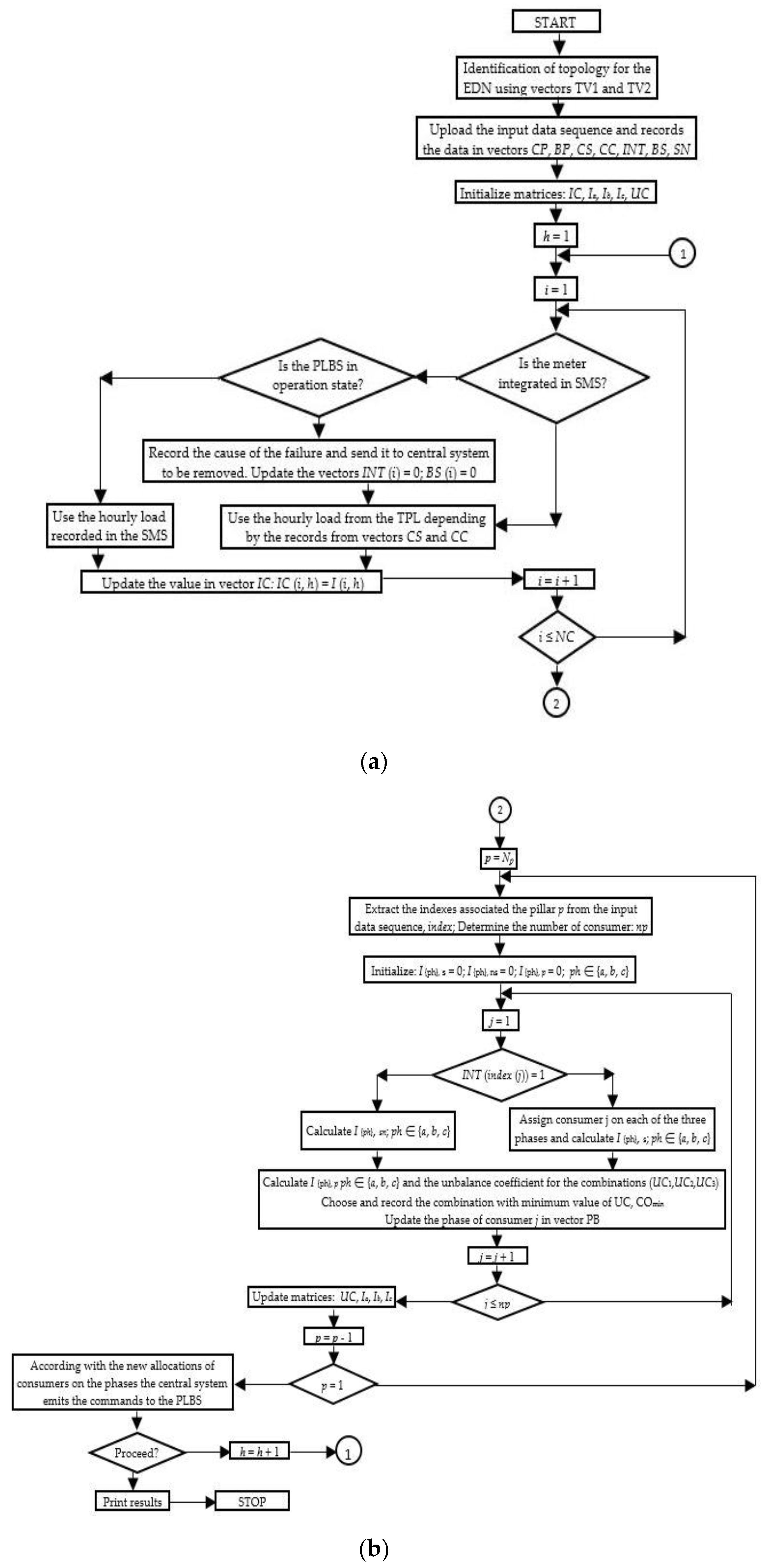
| Step 1. Identification of the topology for the EDN based on the vectors TV1 and TV2, built with the vectors Bi and Be which contain the input and end nodes (pillars) assigned each branch. |
| Step 2. Upload the input data sequence from the database of the DNO corresponding to the SP of EDN: Store the information in the vectors: CP, BP, CS, CC, INT, BS, and SN. Determine the number of consumers supplied: NC = length (SN); Initialize the matrices IC ∈ ℝ*(Nc×H), Ia, Ib, and Ic ∈ ℝ* (Np×H), and UC∈ ℝ*(Np×H) for each hour h, h = 1…H Set initial consumer index: i = 0; while i ≤ Nc Increase consumer index: i = i + 1; if INT (i, h) = 1 if BS (i, h) = 1 Update IC (i, h) with the value recorded on the line SN(i) and column h of the consumption matrix loaded from the SMS; else Send a warning message to the central system on the failure/missing communication of PLBD to be repaired as soon as possible; Update IC (i, h) with the assigned value from the TLP depending the records from the vectors CS (i) and CC (i), day (weekend or working), and season (springer, summer, autumn, or winter); else Update IC (i, h) with the assigned value from the TLP depending the records from the vectors CS (i) and CC (i), day (weekend or working), and season (springer, summer, autumn, or winter); |
| Step 3. The PLB sequence at the level of each pillar: Set initial pillar index: p = Np; while (p ≥ 1) and (p ≤ Np) Initialize the vector index; Find the index corresponding to pillar p in vector CP, and store in vector index; Determine the number of consumers connected at the pillar p: np = length (index); Initialize the sums of phase currents corresponding to: switchable consumers: Ias = 0, Ibs = 0, Ics = 0; non-switchable consumers: Ians = 0, Ibns = 0, Icns = 0; all consumers: Iap = 0, Ibp = 0, Icp = 0; Set initial consumer index: j = 0; while j ≤ np Increase consumer index: j = j + 1; if (INT(index (j)) = 0) and (BP (index (j)) = {a}) Update sum of current to non-switchable consumers on the phase a: Ians = Ians + IC (index (j)); if BP (index (j)) = {b}) Update sum of current to non-switchable consumers on the phase b: Ibns = Ibns + IC (index(j)); else Update sum of current to non-switchable consumers on the phase c: Icns = Icns + IC (index (j)); if (INT(index (j)) = 1) and (BS (index (j)) = 0) Changing the category of consumer j from switchable in non-switchable; if (BP (index (j)) = {a}) Update sum of current to non-switchable consumers on the phase a: Ians = Ians + IC (index (j)); if BP (index (j)) = {b}) Update sum of current to non-switchable consumers on the phase b: Ibns = Ibns + IC (index (j)); else Update sum of current to non-switchable consumers on the phase c: Icns = Icns + IC (index (j)); if (INT(index (j)) = 1) and (BS (index (j)) = 1) Assigning the consumer j on each of the three phases: case Combination 1 – allocation of the consumer j on the phase a Compute the fictive sum of phase currents to switchable consumers: Iasf1 = Ias + IC (index (j)); Ibsf1 = Ibs; Icsf1 = Ics; Compute the fictive sum of the phase currents to all consumers: Iapf1 = Ians + Iasf1; Ibpf1= Ibns + Ibsf1; Icpf1 = Icns + Icsf1; Compute the average value of the phase currents, Iaverage1 (rel. (3)) Compute the UC1 (rel. (2)); case Combination 2 – allocation of the consumer j on the phase b Compute the fictive sum of phase currents to switchable consumers: Iasf2 = Ias; Ibsf2 = Ibs + IC (index (j)); Icsf2 = Ics; Compute the fictive sum of the phase currents to all consumers: Iapf2 = Ians + Iasf2; Ibpf2 = Ibns + Ibsf2; Icpf2 = Icns + Icsf2; Compute the average value of the phase currents, Iaverage2, (rel. (3)); Compute the UC2 (rel. (2)); case Combination 3 – allocation of the consumer j on the phase c Compute the fictive sum of phase current to switchable consumers: Iasf3 = Ias; Ibsf3 = Ibs; Icsf3 = Ics + IC (index (j)); Compute the fictive sum of the phase currents of all consumers: Iapf3 = Ians + Iasf3; Ibpf3 = Ibns + Ibsf3; Icpf3 = Icns + Icsf3; Compute the average value of the phase currents, Iaverage3 (rel. (3)); Compute the UC3 (rel. (2)); Determine the minimum value of UC: min (UC1, UC2, UC3); Store the number of combination with UCmin, COmin, corresponding to one of the three phase: if COmin = 1 Update in the vector PB the phase a: PB (index (j)) = {a}; Update the sum of phase currents to switchable consumers: Ias = Iasf1; Ibs = Ibsf1; Ics = Icsf1; Update the sum of phase currents to all consumers: Iap = Iapf1; Ibp = Ibpf1; Icp = Icpf1; if COmin = 2 Update in the vector PB the phase b: PB(index (j)) = {b}; Update the sum of phase currents to switchable consumers: Ias = Ias2; Ibs = Ibsf2; Ics = Icsf2; Update the sum of phase currents to all consumers: Iap = Iapf2; Ibp = Ibpf2; Icp = Icpf2; else Update in the vector PB the phase c: PB(index (j)) = {c}; Update the sum of phase currents to switchable consumers: Ias = Ias3; Ibs = Ibsf3; Ics = Icsf3; Update the sum of phase currents to all consumers: Iap = Iapf3; Ibp = Ibpf3; Icp = Icpf3; Update the value of unbalanced coefficient UC (p, h) = UCmin; Update the value of phase currents Ia (p, h) = Iap, Ib (p, h) = Ibp, and Ic (p, h) = Icp; Decrease pillar index: p = p − 1; According with the new allocations from vector PB the central system emits the instructions at each PLBD; Increase hour index: h = h + 1; Print results: UC, Ia, Ib, Ic. |
| Branch | Type Conductor | Cross-Section of Phase Conductors [mm2] | Cross-Section of Neutral Conductor [mm2] | Length [km] | r0 [Ω/km] | x0 [Ω/km] |
|---|---|---|---|---|---|---|
| SP-11 | Classic | 50 | 50 | 0.160 | 0.61 | 0.298 |
| 11–15 | Classic | 50 | 50 | 0.160 | 0.61 | 0.298 |
| 11–95 | Classic | 50 | 50 | 1.960 | 0.61 | 0.298 |
| 15–27 | Classic | 35 | 35 | 0.480 | 0.871 | 0.055 |
| 15–39 | Classic | 35 | 35 | 0.480 | 0.871 | 0.055 |
| 37–46 | Classic | 25 | 25 | 0.280 | 1.235 | 0.319 |
| Total | 50 | 50 | 2.280 | 0.61 | 0.298 | |
| 35 | 35 | 0.960 | 0.871 | 0.055 | ||
| 25 | 25 | 0.280 | 1.235 | 0.319 | ||
| Total | 3.520 | |||||
| Consumer’ Type | Initial Phase | Consumption SECTOR | |||||||
|---|---|---|---|---|---|---|---|---|---|
| 1-P | 3-P | a | b | c | abc | I | II | III | IV |
| 161 | 2 | 42 | 72 | 47 | 2 | 161 | 2 | - | - |
| Hour | Ia [A] | Ib [A] | Ic [A] | I0 [A] | UC |
|---|---|---|---|---|---|
| 1 | 14.77 | 48.71 | 19.47 | 31.84 | 1.29 |
| 2 | 14.01 | 46.55 | 18.64 | 30.49 | 1.30 |
| 3 | 13.24 | 43.81 | 17.73 | 28.58 | 1.29 |
| 4 | 13.36 | 44.40 | 17.45 | 29.20 | 1.30 |
| 5 | 13.55 | 43.94 | 17.99 | 28.43 | 1.28 |
| 6 | 12.38 | 36.47 | 16.98 | 22.15 | 1.23 |
| 7 | 16.73 | 41.58 | 19.49 | 23.59 | 1.18 |
| 8 | 19.53 | 45.17 | 20.93 | 24.97 | 1.17 |
| 9 | 19.69 | 49.91 | 21.88 | 29.18 | 1.20 |
| 10 | 18.05 | 53.57 | 21.70 | 33.83 | 1.26 |
| 11 | 19.21 | 61.57 | 23.16 | 40.52 | 1.30 |
| 12 | 17.44 | 58.17 | 20.53 | 39.28 | 1.33 |
| 13 | 17.94 | 61.76 | 21.40 | 42.20 | 1.35 |
| 14 | 17.87 | 60.11 | 22.35 | 40.18 | 1.32 |
| 15 | 17.91 | 61.07 | 22.21 | 41.18 | 1.33 |
| 16 | 15.99 | 54.16 | 21.22 | 35.84 | 1.31 |
| 17 | 18.38 | 61.07 | 22.53 | 40.77 | 1.32 |
| 18 | 21.55 | 66.87 | 25.80 | 43.34 | 1.29 |
| 19 | 21.31 | 59.27 | 25.14 | 36.19 | 1.23 |
| 20 | 21.27 | 51.86 | 23.77 | 29.41 | 1.18 |
| 21 | 25.66 | 58.78 | 27.08 | 32.43 | 1.17 |
| 22 | 27.69 | 68.53 | 31.57 | 39.04 | 1.19 |
| 23 | 24.83 | 69.17 | 30.67 | 41.72 | 1.22 |
| 24 | 17.12 | 53.18 | 23.17 | 33.45 | 1.26 |
| Hour | Main Conductors | Branching Conductors | Total | ||||||
|---|---|---|---|---|---|---|---|---|---|
| a | b | c | Neutral | a | b | c | Neutral | ||
| 1 | 0.03 | 0.54 | 0.11 | 0.43 | 0.003 | 0.014 | 0.001 | 0.011 | 1.14 |
| 2 | 0.03 | 0.49 | 0.10 | 0.39 | 0.003 | 0.013 | 0.001 | 0.011 | 1.04 |
| 3 | 0.02 | 0.43 | 0.09 | 0.35 | 0.002 | 0.011 | 0.001 | 0.009 | 0.92 |
| 4 | 0.02 | 0.44 | 0.09 | 0.35 | 0.002 | 0.012 | 0.001 | 0.010 | 0.93 |
| 5 | 0.02 | 0.44 | 0.09 | 0.35 | 0.002 | 0.011 | 0.001 | 0.010 | 0.93 |
| 6 | 0.02 | 0.31 | 0.08 | 0.25 | 0.002 | 0.006 | 0.001 | 0.006 | 0.67 |
| 7 | 0.04 | 0.41 | 0.11 | 0.32 | 0.005 | 0.007 | 0.001 | 0.008 | 0.90 |
| 8 | 0.05 | 0.50 | 0.12 | 0.38 | 0.007 | 0.009 | 0.001 | 0.011 | 1.08 |
| 9 | 0.05 | 0.59 | 0.14 | 0.46 | 0.007 | 0.012 | 0.001 | 0.013 | 1.27 |
| 10 | 0.04 | 0.66 | 0.13 | 0.52 | 0.005 | 0.017 | 0.001 | 0.015 | 1.40 |
| 11 | 0.05 | 0.87 | 0.15 | 0.68 | 0.006 | 0.025 | 0.001 | 0.021 | 1.81 |
| 12 | 0.04 | 0.77 | 0.12 | 0.60 | 0.005 | 0.025 | 0.001 | 0.020 | 1.58 |
| 13 | 0.04 | 0.86 | 0.13 | 0.68 | 0.005 | 0.029 | 0.001 | 0.023 | 1.77 |
| 14 | 0.04 | 0.82 | 0.14 | 0.65 | 0.005 | 0.025 | 0.001 | 0.020 | 1.71 |
| 15 | 0.04 | 0.85 | 0.14 | 0.67 | 0.005 | 0.026 | 0.001 | 0.021 | 1.76 |
| 16 | 0.04 | 0.67 | 0.13 | 0.53 | 0.004 | 0.019 | 0.001 | 0.015 | 1.40 |
| 17 | 0.05 | 0.85 | 0.15 | 0.67 | 0.005 | 0.026 | 0.001 | 0.021 | 1.76 |
| 18 | 0.06 | 1.04 | 0.19 | 0.82 | 0.007 | 0.028 | 0.002 | 0.024 | 2.17 |
| 19 | 0.06 | 0.84 | 0.18 | 0.66 | 0.007 | 0.017 | 0.002 | 0.017 | 1.78 |
| 20 | 0.06 | 0.66 | 0.16 | 0.51 | 0.007 | 0.011 | 0.001 | 0.013 | 1.43 |
| 21 | 0.09 | 0.87 | 0.21 | 0.68 | 0.012 | 0.014 | 0.002 | 0.018 | 1.89 |
| 22 | 0.10 | 1.18 | 0.29 | 0.93 | 0.012 | 0.019 | 0.002 | 0.022 | 2.55 |
| 23 | 0.08 | 1.17 | 0.27 | 0.93 | 0.009 | 0.021 | 0.002 | 0.021 | 2.51 |
| 24 | 0.04 | 0.66 | 0.15 | 0.53 | 0.004 | 0.014 | 0.001 | 0.012 | 1.42 |
| Total | 1.13 | 16.93 | 3.48 | 13.34 | 0.130 | 0.408 | 0.028 | 0.370 | 35.81 |
| Hour | Ia [A] | Ib [A] | Ic [A] | I0 [A] | UC |
|---|---|---|---|---|---|
| 1 | 27.56 | 27.50 | 27.82 | 0.30 | 1.0000 |
| 2 | 26.25 | 26.53 | 26.37 | 0.24 | 1.0000 |
| 3 | 24.88 | 25.03 | 24.82 | 0.19 | 1.0000 |
| 4 | 25.29 | 24.88 | 24.99 | 0.36 | 1.0000 |
| 5 | 25.22 | 25.01 | 25.21 | 0.21 | 1.0000 |
| 6 | 21.47 | 22.69 | 21.65 | 1.14 | 1.0006 |
| 7 | 24.77 | 24.68 | 28.31 | 3.58 | 1.0042 |
| 8 | 31.90 | 26.76 | 26.93 | 5.06 | 1.0070 |
| 9 | 28.83 | 29.06 | 33.54 | 4.59 | 1.0050 |
| 10 | 30.66 | 30.78 | 31.81 | 1.10 | 1.0003 |
| 11 | 34.76 | 34.55 | 34.53 | 0.22 | 1.0000 |
| 12 | 32.61 | 31.65 | 31.78 | 0.91 | 1.0002 |
| 13 | 33.25 | 34.50 | 33.23 | 1.26 | 1.0003 |
| 14 | 33.91 | 33.04 | 33.29 | 0.77 | 1.0001 |
| 15 | 33.49 | 34.20 | 33.40 | 0.76 | 1.0001 |
| 16 | 30.88 | 30.23 | 30.18 | 0.68 | 1.0001 |
| 17 | 33.72 | 34.38 | 33.77 | 0.64 | 1.0001 |
| 18 | 38.43 | 37.96 | 37.71 | 0.63 | 1.0001 |
| 19 | 37.69 | 34.07 | 33.87 | 3.72 | 1.0025 |
| 20 | 30.67 | 30.70 | 35.48 | 4.79 | 1.0049 |
| 21 | 34.87 | 41.56 | 35.03 | 6.61 | 1.0070 |
| 22 | 40.63 | 46.86 | 40.21 | 6.46 | 1.0051 |
| 23 | 39.94 | 40.25 | 44.37 | 4.29 | 1.0024 |
| 24 | 31.96 | 30.73 | 30.71 | 1.24 | 1.0004 |
| Hour | Main Conductors | Branching Conductors | Total | ||||||
|---|---|---|---|---|---|---|---|---|---|
| a | b | c | Neutral | a | b | c | Neutral | ||
| 1 | 0.12 | 0.13 | 0.14 | 0.01 | 0.00 | 0.01 | 0.01 | 0.01 | 0.43 |
| 2 | 0.11 | 0.13 | 0.12 | 0.01 | 0.00 | 0.01 | 0.01 | 0.01 | 0.39 |
| 3 | 0.10 | 0.12 | 0.10 | 0.01 | 0.00 | 0.01 | 0.00 | 0.01 | 0.35 |
| 4 | 0.12 | 0.10 | 0.10 | 0.01 | 0.01 | 0.01 | 0.00 | 0.01 | 0.35 |
| 5 | 0.11 | 0.11 | 0.10 | 0.01 | 0.01 | 0.00 | 0.00 | 0.01 | 0.35 |
| 6 | 0.08 | 0.08 | 0.08 | 0.00 | 0.00 | 0.00 | 0.00 | 0.01 | 0.26 |
| 7 | 0.11 | 0.11 | 0.13 | 0.01 | 0.00 | 0.00 | 0.01 | 0.01 | 0.37 |
| 8 | 0.17 | 0.12 | 0.13 | 0.01 | 0.01 | 0.00 | 0.00 | 0.01 | 0.45 |
| 9 | 0.17 | 0.13 | 0.18 | 0.01 | 0.01 | 0.00 | 0.01 | 0.01 | 0.52 |
| 10 | 0.15 | 0.17 | 0.17 | 0.01 | 0.01 | 0.01 | 0.01 | 0.01 | 0.54 |
| 11 | 0.22 | 0.20 | 0.20 | 0.01 | 0.01 | 0.01 | 0.01 | 0.02 | 0.68 |
| 12 | 0.19 | 0.16 | 0.17 | 0.01 | 0.01 | 0.01 | 0.01 | 0.02 | 0.59 |
| 13 | 0.17 | 0.23 | 0.19 | 0.02 | 0.01 | 0.02 | 0.01 | 0.02 | 0.66 |
| 14 | 0.21 | 0.19 | 0.18 | 0.01 | 0.01 | 0.01 | 0.01 | 0.02 | 0.64 |
| 15 | 0.17 | 0.22 | 0.19 | 0.01 | 0.01 | 0.01 | 0.01 | 0.02 | 0.65 |
| 16 | 0.17 | 0.15 | 0.16 | 0.01 | 0.01 | 0.01 | 0.01 | 0.01 | 0.52 |
| 17 | 0.17 | 0.22 | 0.20 | 0.01 | 0.01 | 0.01 | 0.01 | 0.02 | 0.66 |
| 18 | 0.23 | 0.27 | 0.24 | 0.01 | 0.01 | 0.01 | 0.01 | 0.02 | 0.82 |
| 19 | 0.22 | 0.22 | 0.19 | 0.01 | 0.01 | 0.01 | 0.01 | 0.02 | 0.69 |
| 20 | 0.16 | 0.18 | 0.20 | 0.01 | 0.00 | 0.01 | 0.01 | 0.01 | 0.58 |
| 21 | 0.21 | 0.29 | 0.22 | 0.02 | 0.00 | 0.02 | 0.01 | 0.02 | 0.78 |
| 22 | 0.28 | 0.35 | 0.32 | 0.02 | 0.00 | 0.02 | 0.01 | 0.02 | 1.01 |
| 23 | 0.30 | 0.28 | 0.32 | 0.01 | 0.01 | 0.01 | 0.01 | 0.02 | 0.96 |
| 24 | 0.16 | 0.18 | 0.16 | 0.01 | 0.00 | 0.01 | 0.01 | 0.01 | 0.54 |
| Total | 4.09 | 4.34 | 4.18 | 0.26 | 0.15 | 0.20 | 0.19 | 0.36 | 13.76 |
| No. | Algorithm | Computational Times [Seconds] |
|---|---|---|
| 1 | SMD (Proposed) | 1.26 |
| 2 | MCLA | 0.58 |
| 3 | PSO | 348 |
| 4 | GA | 291 |
| No. | Algorithm | Characteristics of EDN | UCinitial | UCfinal | Improvement [%] |
|---|---|---|---|---|---|
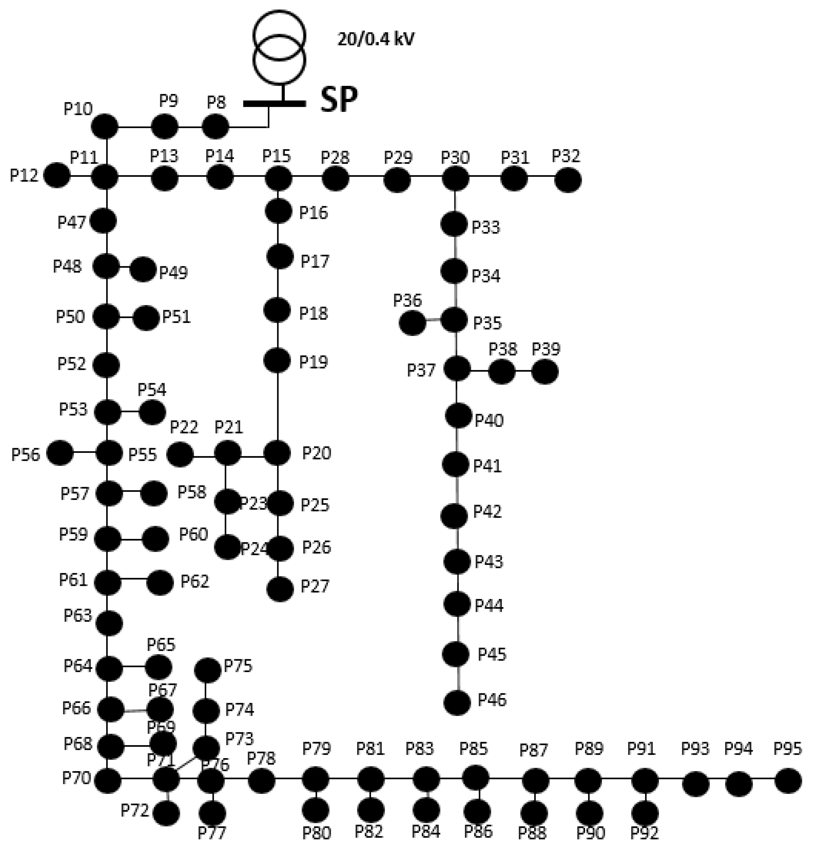
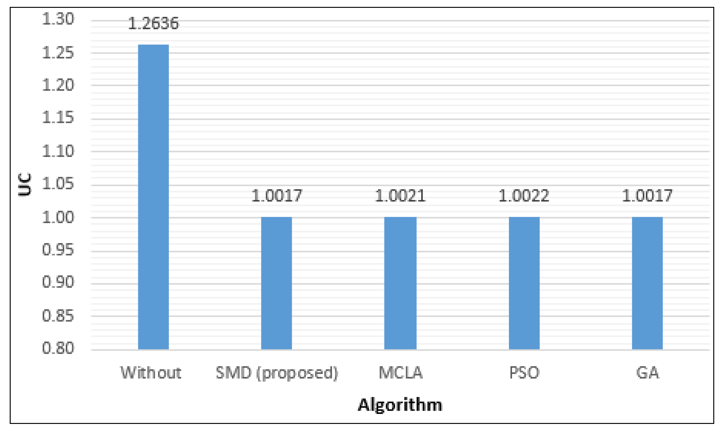
| 1 | SMD (Proposed) | real/complex/88 nodes/163 consumers | 1.26 | 1.0017 | 25.8 |
| 2 | BBA | fictive/radial without lateral branches/51 consumers | 1.17 | 1.07 | 9.4 |
| 3 | MIP | fictive/radial with 2 lateral branches/6 nodes | 1.086 | 1.005 | 8.0 |
| Algorithm | Main Conductors | Branching Conductors | Total | δΔW [%] | ||||||
|---|---|---|---|---|---|---|---|---|---|---|
| a | b | c | Neutral | a | b | c | Neutral | |||
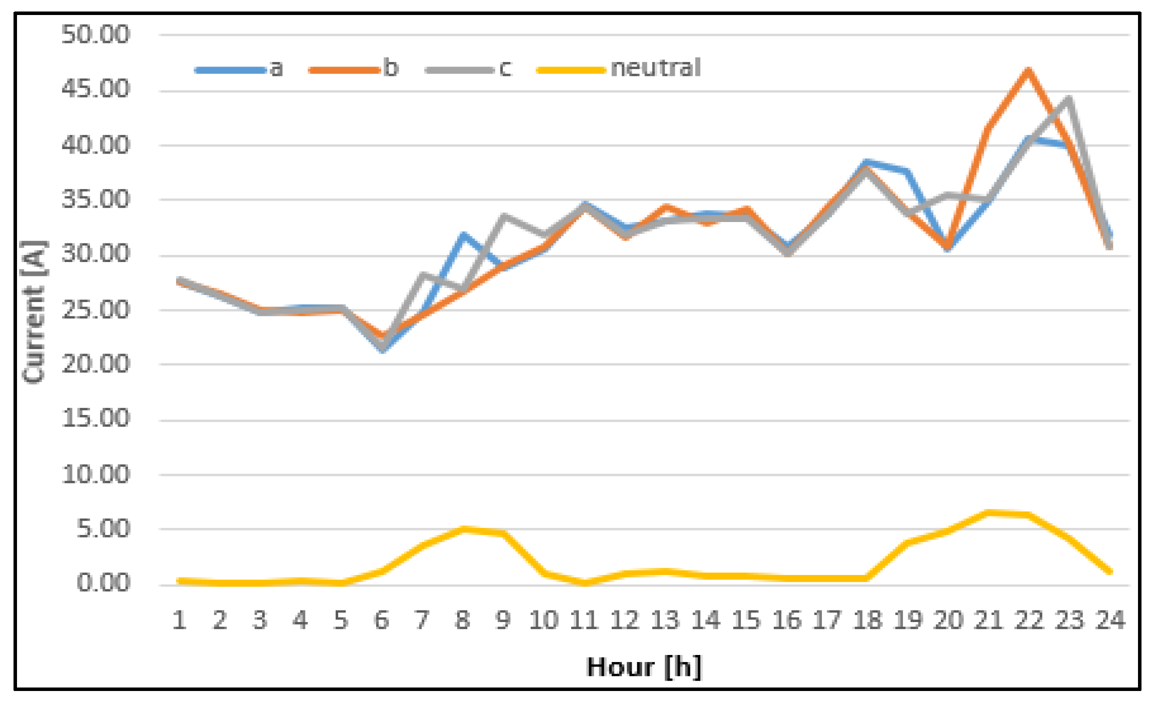
| Without | 1.13 | 16.93 | 3.48 | 13.34 | 0.13 | 0.41 | 0.03 | 0.37 | 35.81 | - |
| SMD (proposed) | 4.09 | 4.34 | 4.18 | 0.26 | 0.15 | 0.20 | 0.19 | 0.36 | 13.76 | 61.57 |
| MCLA | 4.14 | 6.23 | 4.98 | 4.32 | 0.33 | 0.05 | 0.16 | 0.36 | 20.57 | 42.56 |
| PSO | 4.44 | 4.43 | 3.77 | 0.32 | 0.23 | 0.17 | 0.15 | 0.36 | 13.86 | 61.30 |
| GA | 3.66 | 4.62 | 4.50 | 0.51 | 0.14 | 0.19 | 0.21 | 0.36 | 14.19 | 60.37 |
| Algorithm | Phase | ||
|---|---|---|---|
| a | b | c | |
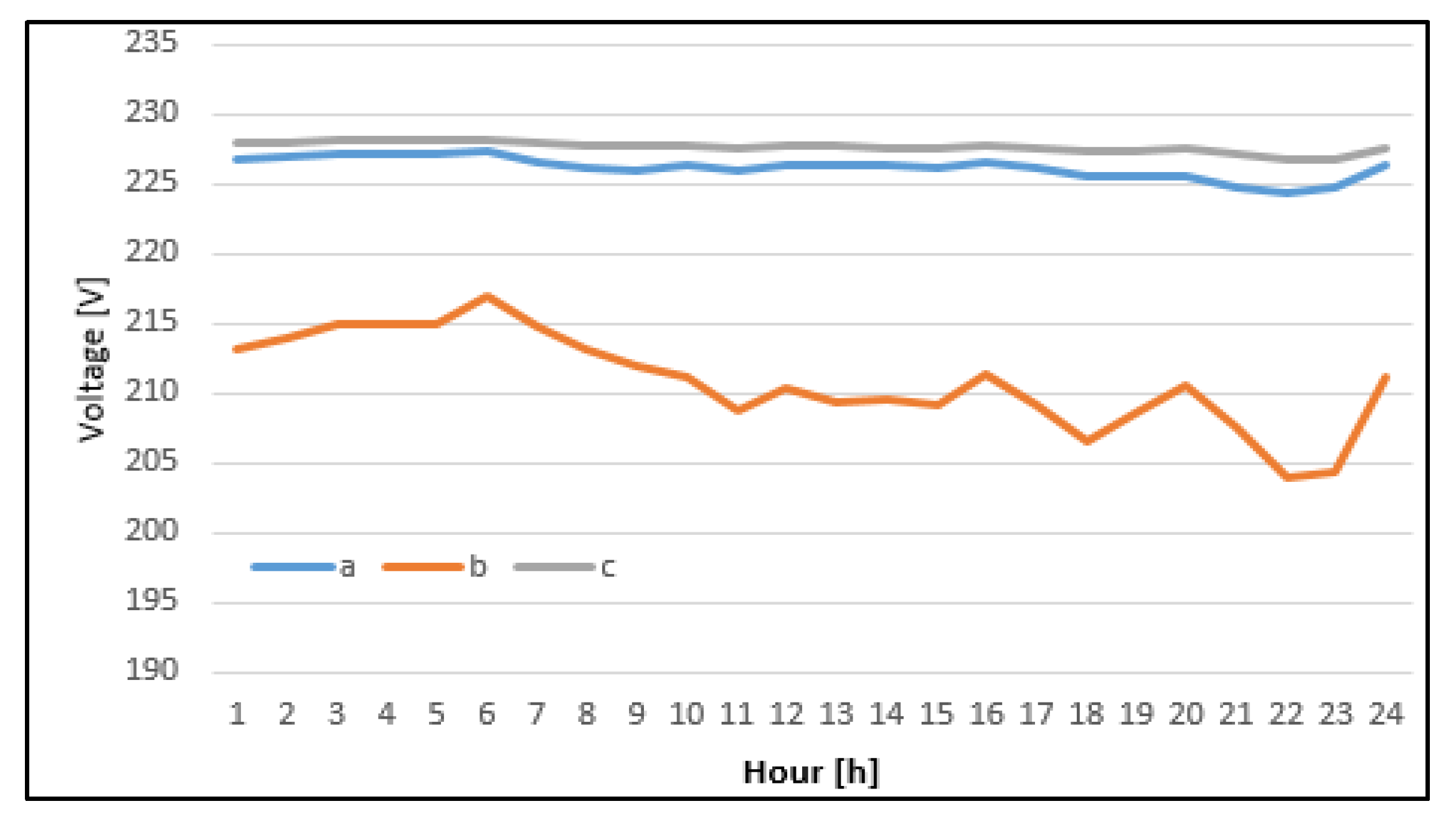
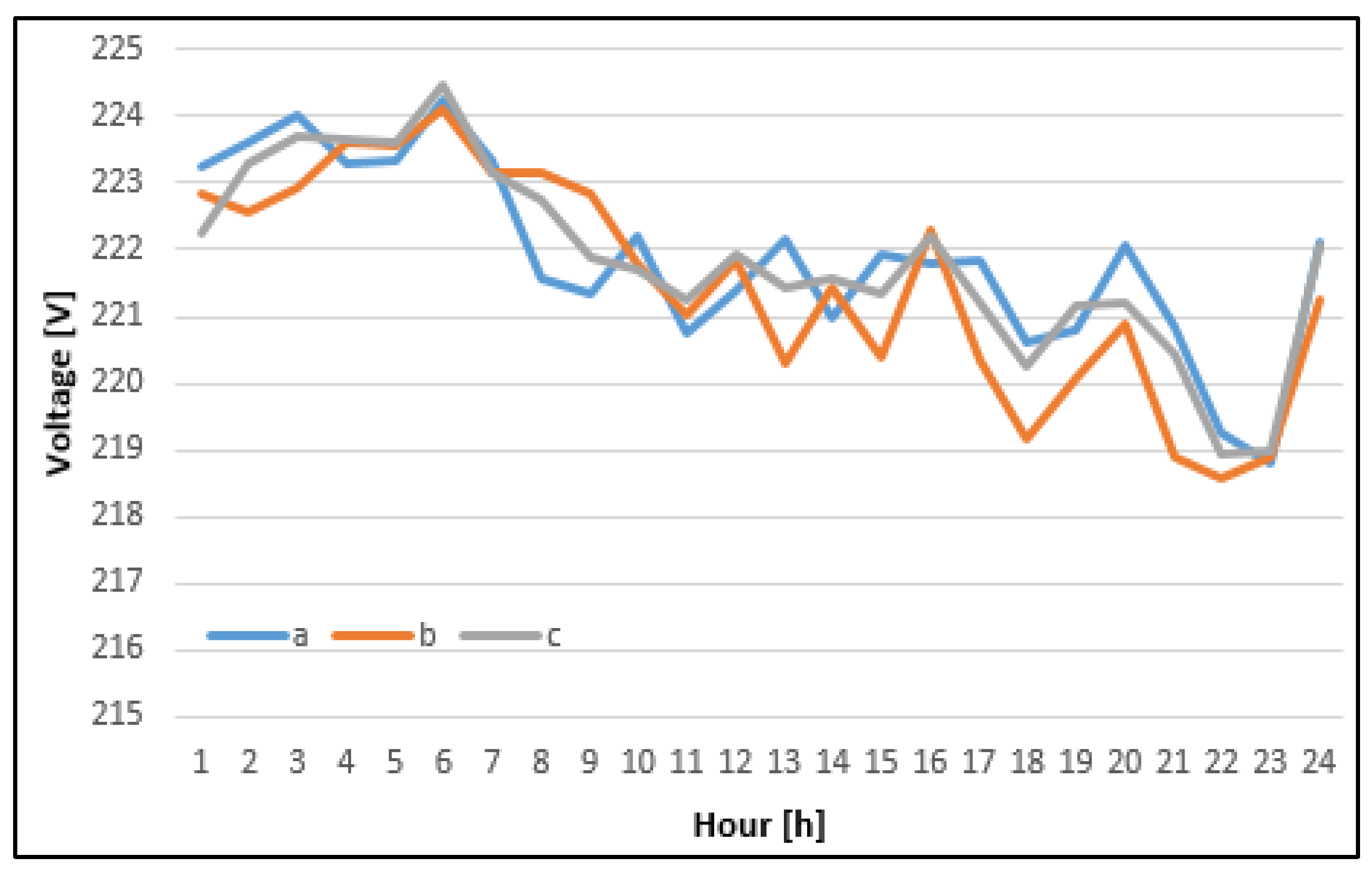
| Without | 224.33 | 204.00 | 226.71 |
| SMD (proposed) | 218.81 | 218.58 | 218.94 |
| MCLA | 218.90 | 211.59 | 224.49 |
| PSO | 218.19 | 219.03 | 218.55 |
| GA | 219.41 | 217.28 | 219.07 |
© 2020 by the authors. Licensee MDPI, Basel, Switzerland. This article is an open access article distributed under the terms and conditions of the Creative Commons Attribution (CC BY) license (http://creativecommons.org/licenses/by/4.0/).
Share and Cite
Grigoraș, G.; Neagu, B.-C.; Gavrilaș, M.; Triștiu, I.; Bulac, C. Optimal Phase Load Balancing in Low Voltage Distribution Networks Using a Smart Meter Data-Based Algorithm. Mathematics 2020, 8, 549. https://doi.org/10.3390/math8040549
Grigoraș G, Neagu B-C, Gavrilaș M, Triștiu I, Bulac C. Optimal Phase Load Balancing in Low Voltage Distribution Networks Using a Smart Meter Data-Based Algorithm. Mathematics. 2020; 8(4):549. https://doi.org/10.3390/math8040549
Chicago/Turabian StyleGrigoraș, Gheorghe, Bogdan-Constantin Neagu, Mihai Gavrilaș, Ion Triștiu, and Constantin Bulac. 2020. "Optimal Phase Load Balancing in Low Voltage Distribution Networks Using a Smart Meter Data-Based Algorithm" Mathematics 8, no. 4: 549. https://doi.org/10.3390/math8040549
APA StyleGrigoraș, G., Neagu, B.-C., Gavrilaș, M., Triștiu, I., & Bulac, C. (2020). Optimal Phase Load Balancing in Low Voltage Distribution Networks Using a Smart Meter Data-Based Algorithm. Mathematics, 8(4), 549. https://doi.org/10.3390/math8040549