Abstract
With improved measurement and modelling technology, variability has emerged as an essential feature in non-equilibrium processes. While traditionally, mean values and variance have been heavily used, they are not appropriate in describing extreme events where a significant deviation from mean values often occurs. Furthermore, stationary Probability Density Functions (PDFs) miss crucial information about the dynamics associated with variability. It is thus critical to go beyond a traditional approach and deal with time-dependent PDFs. Here, we consider atmospheric data from the Whole Atmosphere Community Climate Model (WACCM) and calculate time-dependent PDFs and the information length from these PDFs, which is the total number of statistically different states that a system evolves through in time. Specifically, we consider the three cases of sampling data to investigate the distribution of information (information budget) along the altitude and longitude to gain a new perspective of understanding variabilities, correlation among different variables and regions. Time-dependent PDFs are shown to be non-Gaussian in general; the information length tends to increase with the altitude albeit in a complex form; this tendency is more robust for flows/shears than temperature. Much similarity among flows and shears in the information length is also found in comparison with the temperature. This means a strong correlation among flows/shears because of their coupling through gravity waves in this particular WACCM model. We also find the increase of the information length with the latitude and interesting hemispheric asymmetry for flows/shears/temperature, with the tendency of anti-correlation (correlation) between flows/shears and temperature at high (low) latitude. These results suggest the importance of high latitude/altitude in the information budget in the Earth’s atmosphere, the spatial gradient of the information length being a useful proxy for information flow.
1. Introduction
With improved measurement and modelling technology, variability has emerged as an essential feature in non-equilibrium processes. Closely linked to unpredictability, variability plays a crucial role in various unexpected or undesirable events such as fusion plasma eruption, extreme weather conditions, stock market crash, etc. [1,2,3,4,5,6,7,8,9,10,11,12,13,14,15,16,17,18,19,20,21]. Specifically, anomalous (much larger than mean values) transport associated with large fluctuations in fusion plasmas can degrade the confinement, potentially even terminating fusion operation [3]. Tornadoes are rare, large amplitude events, but can cause very substantial damage when they do occur. Furthermore, gene expression and protein productions, which used to be thought of as smooth processes, have also been observed to occur in bursts (e.g., [16,17,18,19,20]).
How to quantify variability mathematically, however, does not seem to be well established. For unpredictable events, we use a Probability Density Function (PDF) to describe the likelihood of a certain event to take place. A simplest and popular example is Gaussian PDF which has the nice property of symmetry and uniquely being defined by only two parameters—the mean value for the peak position and standard deviation for the width of a PDF. Note that the variance is the square of standard deviation. As a broad PDF has a wide range of values for a finite probability, suggesting less predictability, variability can mean a large variance. On the other hand, the temporal change in mean value is also used as a measure of variability. How do we then treat the case where variance increases or decreases in time? Furthermore, for a non-Gaussian PDF, we also need to consider the change in other characteristics like symmetry, skewness, or kurtosis, and all other higher moments. This is especially important for extreme events noted above since the assumption of small fluctuations with short correlation time for the Gaussian PDF badly fails, with a very limited utility of mean value and variance.
In particular, mean value does not give the mostly likely value (the peak position) when there is more than one peak. In the case of a PDF with one peak as in the case of gamma distributions [22], the mean value could be a useful proxy of the mostly likely value; however, even when the initial and final distributions are gamma distributions, the time-evolution in the intermediate time does not necessarily satisfy gamma distribution [23]. Furthermore, for the given initial and final PDFs, there is an infinite number of different paths that a PDF can take in evolving from the initial to the final PDF out of equilibrium. It is this path-dependence that can be important for characterizing the true dynamical changes out of equilibrium such as hysteresis in phase transition [24]. This brings us the importance of considering the entire PDF and their time evolution in defining variability. This is especially important for extreme events where a significant deviation from mean values often occurs.
Information length—In our previous work, we showed that time-dependent PDFs provide a key insight that is completely missing in any studies using only mean values, variance or stationary PDFs. Specifically, we quantify the similarity and disparity between PDFs by assigning the metric between the two such that the distance between two PDFs increases with the disparity between them [25,26]. For Gaussian PDFs, a statistically different state is attained when the physical distance exceeds the resolution set by the uncertainty (PDF width). We extended this concept to time-dependent problems where a PDF changes continuously in time and introduced the information length to quantify the number of statistically different states that a system evolves through in time to reach time t starting from an initial PDF at time 0 [24,27,28,29,30,31,32,33,34,35,36]. One of the merits of is that it is invariant under the (time-independent) change of variables and thus can be directly compared between different variables unlike physical variables that have different units; for instance, can be used to quantify the correlation between different variables (e.g., [34]) as explained below.
Rigorously, can be shown to be related to the sum of the infinitesimal relative entropy along the trajectory of the system [33,35] (see Appendix A). It is, however, instructive to consider defining (i) a dynamical time scale as the rate of information change and then (ii) by measuring the clock time t by . For example, for a time dependent PDF , is calculated as
From Equation (1), we can see that the dimension of is time and serves as a dynamical time unit for information change. is the total information change between time 0 and t:
The integral in Equation (2) is necessary since in Equation (1) depends on time in general. To understand this, we can consider an oscillator with the characteristic time scale given by its period s. Then, within the clock time 10 s, the number of five oscillations would correspond to the information length 5. In the case where the period varies with time, what is required is the integral of over the time.
When the parameters () of are known, Equation (1) can be related to Fisher information metric ()
Note that, as long as a PDF changes in time, keeps increasing. Only in the relaxation problem when a PDF settles into an equilibrium distribution in the long time limit, approaches a finite value . As a measure of the information change, was shown to map out an attractor structure [30,32,33,35]. In particular, in the case of a stable equilibrium, the effect of different deterministic forces was demonstrated by the scaling of against the peak position of a narrow initial PDF, the minimum value of occurring at the equilibrium point [32,33]. Furthermore, varies smoothly with the initial conditions (e.g., the distance of an initial PDF from the attractor point). In a sharp contrast, in the case of a chaotic attractor, varies abruptly with the peak position of a narrow initial PDF [30]; this sensitive dependence on initial conditions is reminiscent of a Lyapunov exponent. That is, provides a new way of understanding dynamical systems.
Furthermore, Ref. [34] considered a coupled linear process (driven by dichotomous noise) where the two species switch between the two and thus are strongly coupled. From the time-dependent PDFs, they calculated ’s and other metrics (K-L divergence, mutual information, etc.) of the two species. Interestingly, ’s of the two species undergo the same evolution in time unlike other metrics (see the blue line in Figure 4b,c in [34]). In addition, it was only which captured the linear geometry associated with a linear Gaussian process (see Figure 1 in [34]). Furthermore, Ref. [36] showed that the information length is a novel methodology of assessing the effects of coherent structures and turbulent dynamics in plasma turbulence, e.g., quantifying the decorrelation of the flux between different spatial positions due to coherent structures. Finally, the information length can also be applied to any data such as music (e.g., see [31]) where the information flow in different classical musics (e.g., see [31]) were calculated.
In this work, we apply this method to the National Centre for Atmospheric Research Center (NCAR) Whole Atmosphere Community Climate Model (WACCM) and show the information length as a useful index to measure ‘dynamic variability’ and ‘correlation’. The remainder of this paper is organized as follows. Section 2 provides the analysis of WACCM data. Discussions and Conclusions are provided in Section 3.
2. Earth Atmosphere from the WACCM
The Whole Atmosphere Community Climate Model (WACCM) is a global circulation model which has been developed for the last few decades through an inter-divisional collaboration at the National Center for Atmospheric Research (NCAR). Specifically, it integrates the upper atmospheric modeling of High Altitude Observatory, the middle atmosphere modeling of Atmospheric Chemistry Observations & Modeling, and the tropospheric modeling of Climate & Global Dynamics, using the NCAR Community Earth System Model as a common numerical framework. The WACCM is a comprehensive numerical model, spanning the range of altitude from the Earth’s surface to the thermosphere. The particular data that we analyze are described in details in [37,38]. One of the main aims of [37,38] was to investigate the effect of gravity waves on variability as well as on the global circulation pattern, thermal structure and transport of different species. In order to resolve gravity waves, the high horizontal resolution of km and vertical resolution of scale height were necessary. This amounts to the total number of data 1152 (longitude), 768 (latitude), and 209 (altitude/level) for any fixed time. With one-hour resolution, this means that the total number of one-day data for one variable that need to be stored and processed to calculate time-dependent PDFs is , which is over 4 billions. For this reason, the statistical analysis is performed for one-day worth data on the NCAR super computer, with the focus on variability at different layers, levels, and latitudes.
We are interested in the information budget in the seven layers in the atmosphere covering thermosphere, mesopause, mesosphere, stratopause, stratosphere, tropopause, and troposphere from the top to the bottom of the atmosphere. We consider three different cases of data sampling for PDFs:
- All longitude and latitude data to understand the global information budge at the seven layers.
- All longitude data to understand the information budget across latitude at the seven layers.
- All longitude and latitude data to understand the global information budget at all altitude.
According to the sampling in each case above, we calculate the time-dependent PDFs for the six variables:
- Temperature T.
- Zonal flow U.
- Meridional flow V.
- Vertical shear in zonal flow (zonal shear) .
- Vertical shear in meridional flow (meridional shear) .
- Vertical shear in total flow (total shear) .
2.1. Information Budget at the Seven Layers
We use one day data at all longitude and latitude, and five points in altitude to construct time PDF around the middle point of the seven layers. From the time-dependent PDFs in each case, we calculate mean value and standard deviation as a function of time. Figure 1 shows the evolution of mean value (a1) and standard deviation (a2) of zonal flow U, the evolution of mean value (b1) and standard deviation (b2) of meridional flow V, and the evolution of mean value (c1) and standard deviation (c2) of meridional flow temperature T. Four solid lines represent the four spheres, black, blue, green, and red, representing thermosphere, mesosphere, stratosphere, and troposphere, respectively. Three dashed lines represent the three pauses, blue, green, and red representing mesopause, stratopause and tropopause, respectively. It is noticeable that, in Figure 1, standard deviations of U and V tend to be much larger than mean values at the seven layers. At any fixed time, there is a clear phase shift between U and V at the same level. This is due to the presence of strong gravity waves, driving an almost isotropic turbulence with the phase shift between U and V. In addition, much less change in the mean temperature compared with its standard deviation is observed. However, there is no systematic variation in either mean or standard deviation from the top to the bottom layers of the atmosphere. This is to be contrasted to the behavior of the information length, discussed in detail below.
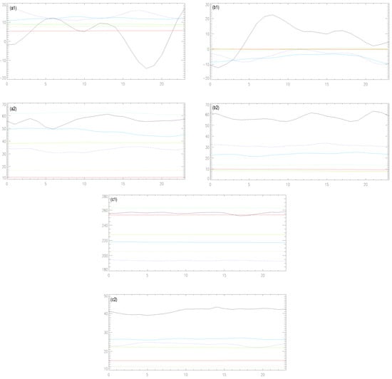
Figure 1.
(a1,a2) are mean value and standard deviation of zonal flow U against time (hours); (b1,b2) are for meridional flow V; (c1,c2) are for temperature T. Four solid lines represent four spheres; black, blue, green and red for thermosphere, mesosphere, stratosphere and troposphere, respectively. Three dashed lines represent three pauses; blue, green, and red for mesopause, stratopause and tropopause, respectively.
In Figure 2, the top left panel shows against time using the same color coding for the seven layers as in Figure 1; four solid lines represent the four spheres, black, blue, green and red representing thermosphere, mesosphere, stratosphere and troposphere, respectively, while three dashed lines represent the three pauses, blue, green, and red representing mesopause, stratopause, and tropopause, respectively. The next seven panels show the snapshots of time-dependent PDFs of zonal flows (different lines representing different times), one panel for each layer. From these, it is clear that PDFs are in general non-Gaussian and non-symmetric.
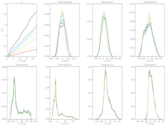
Figure 2.
Top left panel: of zonal flow U against time (hours) where the seven lines represent the seven layers using the same color as in Figure 1; the other seven panels correspond to the seven layers (from thermosphere to troposphere from left/top to right/bottom) where different curves in each panel show the snapshots of time-dependent PDFs of U.
In comparison, the evolution of information length looks much simpler as against t shows roughly a straight line. However, the slope of , which is equal to , is not constant, but varies with time. It is interesting that the largest is seen at the top layer (thermosphere) and that monotonically decreases from the top to the bottom (troposphere).
Equivalent figures are shown for meridional flows V in Figure 3. Compared with PDFs of U, PDFs of V are much narrower and closer to the Gaussian. Nevertheless, of V behaves similarly to of U. In particular, its value decreases monotonically from the top to the bottom layers of the atmosphere. It is also remarkable that the time evolution of is quite similar for U and V at the same layer. This similarity in results from the similar evolution of the time-dependent PDFs of U and V, signifying a strong correlation between U and V due to strong gravity waves (isotropic turbulence), as noted above. The case of temperature T is shown in Figure 4, where we observe quite broad PDFs with more than one peak at some layers. The ordering of of T is a bit different from those of U and V near the top layer while similar near the bottom layer. In addition, for U and V, the largest information gradient is between thermosphere and mesopause. In comparison, for T, the largest information gradient is observed between tropopause and stratopause while thermosphere is well coupled to mesopause with similar .
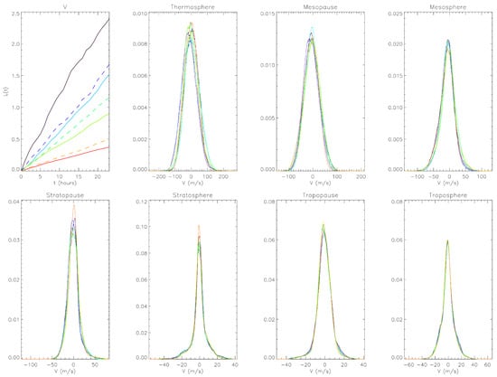
Figure 3.
The same as Figure 2 but for meridional flow V.
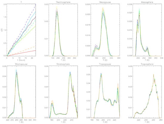
Figure 4.
The same as Figure 2 but for temperature T.
In comparison with Figure 2, Figure 3 and Figure 4, PDFs of zonal shear, meridional shear and total shear all have much simpler shapes with narrower widths (results not shown). The evolution and ordering of of zonal shear, meridional shear and total shear shown in Figure 5 tend to be similar to those of zonal/meridional flows in Figure 2, Figure 3 and Figure 4 although their values are small compared with ’s of flows (due to less change in time-dependent PDFs). More detailed investigation on the dependence of on the altitude is presented in Section 2.3, where is calculated for all pressure levels. We note that we checked on the robustness of our results by using different one-day data and also two-day data of by performing similar analysis. Specifically, we considered different one-day worth data and also two-day worth data, calculated time-dependent PDFs and information lengths, and checked that the information lengths of the different variables behaved similarly to what is presented above.
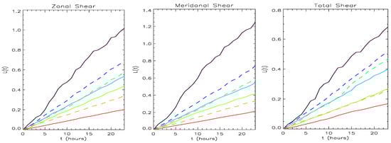
Figure 5.
against time; from the left to right, zonal shear, meridional shear and total shear. The seven lines represent the seven layers using the same color as in Figure 1.
2.2. Information Budget across Latitude
The global information budget—the distribution of information (length) across different layers—studied in Section 2.1 includes the contribution from all different latitudes. In order to understand how the information is distributed across latitude, we now use data from all longitude and five points in each layer for each variable. Figure 6 shows the total against latitude, six panels (a)–(f) corresponding to different variables U, V, T, zonal shear, meridional shear, and total shear, respectively. Each panel contains four solid lines (for spheres) and three dashed lines (for pauses), again using the same color convention as in Figure 1.

Figure 6.
The total information length against latitude (degrees) of U (a), V (b), T (c), zonal shear (d), meridional shear (e), and total shear (f).
For all six variables in Figure 6, the total information length reveals an interesting hemispheric asymmetry. Specifically, except for the bottom layer (troposphere in red color), the information length of U, V, zonal shear, meridional shear, and total shear tends to be larger in the south than in the north. Exactly the opposite tendency is seen in the information length of T. That is, the information length of flows and shears is anti-correlated with temperature. Physically, this may be due to flows/shear flows regulating temperature, reminiscent of turbulence regulation by shear flows [39]. In comparison, at the troposphere, the information length seems to be larger in the north than in the south for all variables, suggesting their correlation.
2.3. Information Budget across Altitude
In Section 2.1–Section 2.2, we calculated PDFs using the data at five points around the middle point of each layer. To map out the information budget across altitude, we now sample the data at all longitude and latitude to calculate time-dependent PDFs and at each altitude classified by the pressure level. Since PDFs now includes only one pressure level, compared with five in Section 2.1, the number of data used to calculate PDFs is five times smaller. This will result in a slightly larger value of (see below).
The total information length at the end of one day against the pressure level is shown in Figure 7c–e for U & V (U in dotted line and V in dashed line), T, and shears (zonal shear in dotted line, meridional shear in dashed line, and total shear in solid line), respectively. The average mean temperature (a) and standard deviation (b) against the pressure level are also shown in Figure 7a,b so that we can identify physical location of three pauses where the temperature gradient is zero. It is noteworthy that the standard deviation can significantly vary over the region where the mean temperature is almost constant. In particular, the standard deviation increases rapidly with the pressure level near the bottom layer.
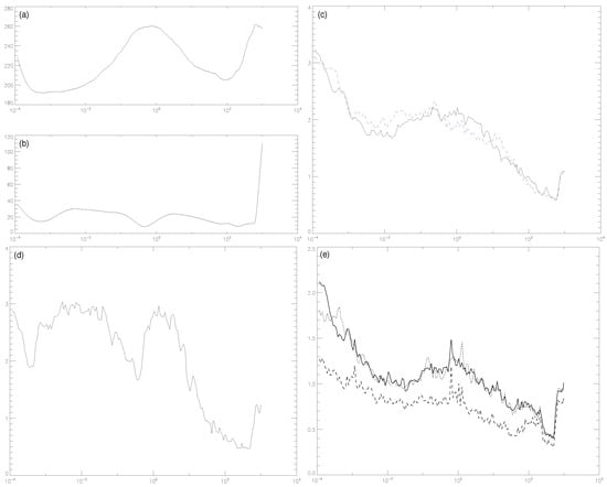
Figure 7.
(a) mean temperature (K) against pressure level (hPa); (b) temperature standard deviation (K) against pressure level (hPa); (c) total information length of U (dotted line) and V (dashed line) against pressure level (hPa); (d) total information length of T against pressure level (hPa); (e) total information length of shears (zonal shear in dotted line, meridional shear in dashed line, and total shear in solid line) against pressure level (hPa). Note that high altitude has low pressure level.
We observe a non-monotonic behavior of of T against pressure level in Figure 7d. Specifically, of T shows three distinct local minima, occurring near (but not exactly at) the three pauses. Interestingly, the local minima of of T in fact seem to coincide with the local minima of the standard deviation of T in Figure 7b. Overall, tends to increase (decrease) as the altitude (pressure level) increases albeit in a complex form due to the presence of the three local minima. This against the pressure level gives us a better understanding of against time for the seven layers shown in Figure 2, Figure 3 and Figure 4. Specifically, the ordering of of T at different layers in Figure 2, Figure 3 and Figure 4 is the manifestation of a non-monotonic behavior of against the pressure level due to these local minima.
The general tendency of increasing with the altitude is also observed for U, V and shears, local minima occurring at the similar pressure level. However, unlike of T, of flow/shears exhibits only two distinct local minima; as the altitude increases, the first local minimum in of U, V and shears occurs between the first two local minima of T while the second local minimum in of U, V and shears seems to coincide with the location of the third local minimum of of T. This suggests the anti-correlation between flows/shears and T nearer the mesosphere while a correlation nearer the troposphere, similar to the behavior that we observed in Figure 6. Furthermore, it is interesting that the two local minima of flows/shears do not occur near the three pauses; of flows/shear at the seven layers in Figure 2, Figure 3 and Figure 4 and Figure 5 yet shows the monotonic increase of with the altitude. Finally, as alluded above, the overall values of in Figure 7 are slightly larger than the corresponding values in Figure 2, Figure 3 and Figure 4 and Figure 5 at the seven layers due to a smaller sample size; the information length increases with the decrease in sample size (see also Section 2.2).
3. Discussion and Conclusions
We investigated time-dependent PDFs and information length for the Earth’s atmosphere data from the global circulation model. Specifically, we analyzed the WACCM model data and calculated time-dependent PDFs as a function of the altitude (pressure level) and the latitude to examine the information budget across different altitudes and latitudes. Time-dependent PDFs were in general non-Gaussian, and the information length calculated from these PDFs shed us a new perspective of understanding variabilities, correlation among different variables and regions. In particular, the information length was found to increase with the altitude albeit in a complex form. The information length of temperature reveals the three local minima coinciding with the location of the local minima of the standard deviation of temperature near the three pauses. In comparison, the information length of zonal flows, meridional flows, zonal shears, zonal shears, and total shears exhibits only two minima. Much similarity in the behavior of the information length among flows and shears in the information length, in comparison with the information length of the temperature, suggests a stronger correlation among flows/shears. This is due to a strong coupling between zonal and meridional flows through gravity waves in this WACCM model.
The correlation between flows/shears and temperature was shown to depend on the altitude, with the tendency of anti-correlation (correlation) between flows/shears and temperature at high (low) altitude. Overall, the information length was found to tend to increase as the latitude increases, with the interesting hemispheric asymmetry for flows/shears/temperature. We conjecture that the information would tend to flow from the region of a higher information length to that of a small information length since a small information length could be due to large entropy while the direction of time follows the entropy-increasing direction. The information flow from higher to lower altitude/latitude in general could then suggest the importance of the high latitude and altitude in the information budget in the Earth’s Atmosphere.
In summary, we demonstrated the utility of the information length as a useful index to understand correlation among different variables and regions as well as information flow.
Author Contributions
Conceptualization, E.K. and H.L.; methodology, E.K., J.H. and H.L.; formal analysis J.H., E.K. and H.L.; software, J.H. and H.L.; writing—original draft preparation, E.K.; writing—review and editing, E.K., H.L. and J.H.; visualization, J.H.; supervision, E.K. and H.L. All authors have read and agreed to the published version of the manuscript.
Funding
This research was in part funded by the Leverhulme Trust Research Fellowship (RF-2018-142-9) and the High Altitude Observatory Visitor Programmes. The APC was funded by Mathematics/MDPI.
Acknowledgments
E.K. acknowledges the Leverhulme Trust Research Fellowship (RF-2018-142-9); E.K. and J.H. acknowledge the High Altitude Observatory Visitor Programmes for their support and are grateful for the hospitality during their one month visit. The National Center for Atmospheric Research is sponsored by the National Science Foundation.
Conflicts of Interest
The authors declare no conflict of interest.
Appendix A. Relation of Equations (1)–(2) and Relative Entropy
Here, we show that and in Equations (1) and (2) are related to the relative entropy (Kullback–Leibler divergence) [32,33]. To this end, we consider two nearby PDFs and at time and and the limit of a very small to do Taylor expansion of by using
By summing for (where ) in the limit , we have
Here, is the information length. Thus, is related to the sum of infinitesimal relative entropy. Note that is a path-dependent, Lagrangian distance between PDFs at time 0 and t and sensitively depends on the particular path that a system passed through reaching the final state. In contrast, the relative entropy depends only on PDFs at time 0 and t and thus does not tell us about intermediate states between initial and final states.
References
- Saw, E.-W.; Kuzzay, D.; Faranda, D.; Guittonneau, A.; Daviaud, F.; Wiertel-Gasquet, C.; Padilla, V.; Dubrulle, B. Experimental characterization of extreme events of inertial dissipation in a turbulent swirling flow. Nat. Commun. 2016, 7, 12466. [Google Scholar] [CrossRef]
- Kim, E.; Diamond, P.H. On intermittency in drift wave turbulence: Structure of the probability distribution function. Phys. Rev. Lett. 2002, 88, 225002. [Google Scholar] [CrossRef]
- Kim, E.; Diamond, P.H. Zonal flows and transient dynamics of the L-H transition. Phys. Rev. Lett. 2003, 90, 185006. [Google Scholar] [CrossRef] [PubMed]
- Kim, E. Consistent theory of turbulent transport in two dimensional magnetohydrodynamics. Phys. Rev. Lett. 2006, 96, 084504. [Google Scholar] [CrossRef] [PubMed]
- Kim, E.; Anderson, J. Structure-based statistical theory of intermittency. Phys. Plasmas 2008, 15, 114506. [Google Scholar] [CrossRef]
- Newton, A.P.L.; Kim, E.; Liu, H.-L. On the self-organizing process of large scale shear flows. Phys. Plasmas 2013, 20, 092306. [Google Scholar] [CrossRef]
- Srinivasan, K.; Young, W.R. Zonostrophic instability. J. Atmos. Sci. 2012, 69, 1633. [Google Scholar] [CrossRef]
- Sayanagi, K.M.; Showman, A.P.; Dowling, T.E. The emergence of multiple robust zonal jets from freely evolving, three-dimensional stratified geostrophic turbulence with applications to Jupiter. J. Atmos. Sci. 2008, 65, 12. [Google Scholar] [CrossRef]
- Tsuchiya, M.; Giuliani, A.; Hashimoto, M.; Erenpreisa, J.; Yoshikawa, K. Emergent self-organized criticality in gene expression dynamics: Temporal development of global phase transition revealed in a cancer cell line. PLoS ONE 2015, 10, e0128565. [Google Scholar] [CrossRef]
- Tang, C.; Bak, P. Mean field theory of self-organized critical phenomena. J. Stat. Phys. 1988, 51, 797. [Google Scholar] [CrossRef]
- Jensen, H.J. Self-organized Criticality: Emergent Complex Behavior in Physical and Biological Systems; Cambridge Univ. Press: Cambridge, UK, 1998. [Google Scholar]
- Pruessner, G. Self-Organised; Criticality Cambridge University Press: Cambridge, UK, 2012. [Google Scholar]
- Longo, G.; Montévil, M. From physics to biology by extending criticality and symmetry breaking. In Progress in Biophysics and Molecular Biology: Systems Biology and Cancer; Pergamon Press: Oxford, UK, 2011; Volume 106, p. 340. [Google Scholar]
- Flynn, S.W.; Zhao, H.C.; Green, J.R. Measuring disorder in irreversible decay processes. J. Chem. Phys. 2014, 141, 104107. [Google Scholar] [CrossRef] [PubMed]
- Nichols, J.W.; Flynn, S.W.; Green, J.R. Order and disorder in irreversible decay processes. J. Chem. Phys. 2015, 142, 064113. [Google Scholar] [CrossRef] [PubMed]
- Ferguson, M.L.; Le Coq, D.; Jules, M.; Aymerich, S.; Radulescu, O.; Declerck, N.; Royer, C.A. Reconciling molecular regulatory mechanisms with noise patterns of bacterial metabolic promoters in induced and repressed states. Proc. Natl. Acad. Sci. USA 2012, 109, 155. [Google Scholar] [CrossRef] [PubMed]
- Shahrezaei, V.; Swain, P.S. Analytical distributions for stochastic gene expression. Proc. Natl. Acad. Sci. USA 2008, 105, 17256. [Google Scholar] [CrossRef]
- Thomas, R.; Torre, L.; Chang, X.; Mehrotra, S. Validation and characterization of DNA microarray gene expression data distribution and associated moments. Bioinformatics 2010, 11, 576. [Google Scholar] [CrossRef] [PubMed]
- Iyer-Biswas, S.; Hayot, F.; Jayaprakash, C. Stochasticity of gene products from transcriptional pulsing. Phys. Rev. E 2009, 79, 031911. [Google Scholar] [CrossRef]
- Elgart, V.; Jia, T.; Fenley, A.T.; Kulkarni, R. Connecting protein and mRNA burst distributions for stochastic models of gene expression. Phys. Biol. 2011, 8, 046001. [Google Scholar] [CrossRef]
- Kim, E.; Liu, H.; Anderson, J. Probability distribution function for self-organization of shear flows. Phys. Plasmas 2009, 16, 052304. [Google Scholar] [CrossRef]
- Feng, X.; Porporato, A.; Rodriguez-Iturbe, I. Stochastic soil water balance under seasonal climates. Proc. R Soc. A 2015, 471, 20140623. [Google Scholar] [CrossRef]
- Kim, E.; Tenkes, L.-M.; Hollerbach, R.; Radulescu, O. Far-from-equilibrium time evolution between two gamma distributions. Entropy 2017, 19, 511. [Google Scholar] [CrossRef]
- Kim, E.; Hollerbach, R. Signature of nonlinear damping in geometric structure of a nonequilibrium process. Phys. Rev. E 2017, 95, 022137. [Google Scholar] [CrossRef]
- Wootters, W.K. Statistical distance and Hilbert space. Phys. Rev. D 1981, 23, 357. [Google Scholar] [CrossRef]
- Frieden, B.R. Physics from Fisher Information; Cambridge University Press: Cambridge, UK, 2000. [Google Scholar]
- Kim, E.; Hollerbach, R. Time-dependent probability density function in cubic stochastic processes. Phys. Rev. E 2016, 94, 052118. [Google Scholar] [CrossRef] [PubMed]
- Hollerbach, R.; Kim, E. Information geometry of non-equilibrium processes in a bistable system with a cubic damping. Entropy 2017, 19, 268. [Google Scholar] [CrossRef]
- Tenkès, L.-M.; Hollerbach, R.; Kim, E. Time-dependent probability density functions and information geometry in stochastic logistic and Gompertz models. J. Stat. Mech. Theory Exp. 2017, 123201. [Google Scholar] [CrossRef]
- Nicholson, S.B.; Kim, E. Investigation of the statistical distance to reach stationary distributions. Phys. Lett. A 2015, 379, 8388. [Google Scholar] [CrossRef]
- Nicholson, S.B.; Kim, E. Structures in sound: Analysis of classical music using the information length. Entropy 2016, 18, 258. [Google Scholar] [CrossRef]
- Heseltine, J.; Kim, E. Novel mapping in non-equilibrium stochastic processes. J. Phys. A 2016, 49, 175002. [Google Scholar] [CrossRef]
- Kim, E.; Lee, U.; Heseltine, J.; Hollerbach, R. Geometric structure and geodesic in a solvable model of nonequilibrium process. Phys. Rev. E 2016, 93, 062127. [Google Scholar] [CrossRef]
- Heseltine, J.; Kim, E. Comparing Information Metrics for a Coupled Ornstein-Uhlenbeck Process. Entropy 2019, 21, 775. [Google Scholar] [CrossRef]
- Kim, E. Investigating Information Geometry in Classical and Quantum Systems through Information Length. Entropy 2018, 20, 574. [Google Scholar] [CrossRef]
- Anderson, J.; Kim, E.; Hnat, B.; Rafiq, T. Elucidating plasma dynamics in Hasegawa-Wakatani turbulence by information geometry. Phys. Plasmas 2020, 27, 022307. [Google Scholar] [CrossRef]
- Liu, H.-L. Large Wind Shears and Their Implications for Diffusion in Regions With Enhanced Static Stability: The Mesopause and the Tropopause. J. Geophys. Res. Atmos. 2017, 122, 9579. [Google Scholar] [CrossRef]
- Liu, H.-L.; McInerney, J.M.; Santos, S.; Lauritzen, P.H.; Taylor, M.A.; Pedatella, N.M. Gravity waves simulated by high-resolution Whole Atmosphere Community Climate Model. Geophys. Res. Lett. 2014, 41, 9106. [Google Scholar] [CrossRef]
- Kim, E. Self-consistent theory of turbulent transport in the solar tachocline; I. Anisotropic turbulence. Astron. Astrophys. 2005, 441, 763. [Google Scholar]
© 2020 by the authors. Licensee MDPI, Basel, Switzerland. This article is an open access article distributed under the terms and conditions of the Creative Commons Attribution (CC BY) license (http://creativecommons.org/licenses/by/4.0/).