Impact of Micro-Scale Stochastic Zonal Flows on the Macro-Scale Visco-Resistive Magnetohydrodynamic Modes

Abstract

A model is developed to simulate micro-scale turbulence driven Zonal Flows (ZFs), and their impact on the Magnetohydrodynamic (MHD) tearing and kink modes is examined. The model is based on a stochastic representation of the micro-scale ZFs with a given Alfvén Mach number, M_S. Two approaches were explored: (i) passive stochastic model where the ZFs amplitudes are independent of the MHD mode amplitude, and (ii) the semi-stochastic model where the amplitudes of the ZFs have a dependence on the amplitude of the MHD mode itself. The results show that the stochastic ZFs can significantly stabilise the (2,1) and (1,1) MHD modes even at very low kinematic viscosity, where the mode is linearly unstable. Our results therefore indicate a possible mechanism for stabilisation of the MHD modes via small-scale perturbations in poloidal flow, simulating the turbulence driven ZFs.

1. Introduction

Establishing and maintaining a stable plasma state in a fusion reactor is an important requirement for achieving fusion power. The complex processes at play in a magnetically confined fusion plasma make it difficult to reach such a stable state. There are various mechanisms which give rise to electromagnetic instabilities in fusion plasmas, that can be detrimental effect on the achievable stable confinement. Two major categories of such mechanisms are the large scale Magnetohydrodynamic (MHD) modes, and the small-scale electromagnetic turbulence perturbations.

The development of MHD instabilities such as $(m=1,n=1)$ internal kink mode [1,2,3,4,5,6,7,8] and/or $(m=1,n=1)$, Tearing Modes (TM) of which a special case for fusion plasmas is the Neoclassical-Tearing Mode (NTM) [9,10,11,12,13,14,15,16] are important limiting factors for establishing a stable confined plasma for long enough time to reach the fusion conditions.

The $(1,1)$ kink mode arises inside the $q=1$ rational surface when q at the axis is $<1$ where q is the safety factor. This mode is observed to trigger the sawtooth oscillations in the plasma core, influencing the confinement quality. Most notable impact of the sawtooth oscillation, is a slow rise of the order of the resistive time scale, in the plasma temperature in the centre, followed by an abrupt crash (on a 100 microsecond time scale), relaxing the temperature profiles back to the initial values at the beginning of each cycle [2,17]. The loss of temperature in the central plasma region limits the achievable pressure profile. However, the sawtooth crash benefits the plasma core confinement by removing the unwanted impurities from the core. Control of the sawtooth crashes for example, their amplitude and frequency, hence would be important for optimising plasma performance in a fusion device [17,18,19,20,21].

The classical $(2,1)$ TM mode can result in the destruction of the topology of the nested magnetic flux surfaces, where the reconnection of the field lines produces magnetic islands in the confined region. The continuous growth of the islands then destroys magnetic confinement and can lead to major disruptions and resulting in production of runaway electrons. A disruption is an event that induces a rapid loss of thermal energy followed by a quench of the plasma current. Disruptions release large heat loads and electromagnetic forces on the surrounding machine structures and can result in a significant damage to the Plasma Facing Components (PFCs) [22,23,24].

Turbulence perturbations on the other hand limit the achievable confinement time by removing the particles and the heat from the confined region via anomalous transport. These small-scale electro-magnetic ion/electron drift waves are ubiquitous in magnetically confined fusion plasmas, and although they do not result directly in a disruption event, they can modify/enhance the large scale MHD modes through non-linear mode coupling and/or the generation of sheared Zonal Flows (ZFs).

In a recent review by Ishizawa and co-authors [25], the findings of an extensive body of work that has been devoted to the study of the multi-scale interactions and the interplay between turbulence and large scale TMs are examined. We will not try to re-examine these works here and will only refer to a summary—destabilisation of TMs through an inverse energy cascade from turbulence perturbations such as small-scale ballooning modes (such as Ion Temperature gradient (ITG), Electron Temperature Gradient (ETG), Kinetic Ballooning Mode (KBM) with twisting parity) or electron Micro-TMs (with tearing parity) have been reported in References [26,27,28,29,30] and References [31,32,33], respectively. This mechanism is observed to affect the stability of the MHD modes either by reducing the stability threshold as compared to pure MHD analysis or by enhancement of the growth rate of the island. Thus, turbulence can create large-scale magnetic islands by the merging of small-scale islands. Other mechanisms such as anomalous current drive by turbulence that is, much like a small-scale dynamo effect [34], or turbulence-driven polarisation current as the result of turbulence-generated ZFs following the reconnected field lines of the island [35], have also been suggested as drivers of magnetic seed islands.

The back reaction of the magnetic islands on the turbulence is expressed through a direct energy cascade from MHD modes to turbulence as a result of the non-linear mode coupling observed in EAST tokamak [36]. Moreover the magnetic perturbation of the field lines, especially around the X-point of the island increases the turbulence outside the island [23], while the coherent vortex flows generated by the interactions between the turbulence and MHD mode at the boundary can act as a transport barrier that leads to suppression of the drift-wave instabilities inside the island [35,37,38,39,40,41,42]. The enhancement of the turbulence outside, and its reduction inside the island, along with the parallel transport results in increased flux which flattens (not completely) the temperature profile inside the separatrix of the island. This flattening of the temperature profile, changes the resistivity inside the island and further reduces the perturbed bootstrap current which has a destabilising effect on the island. It increases the growth of the island and eventually the degradation of the confinement outside the island equilibrates the profiles inside and outside leading to its saturation at lower plasma stored energy [42,43].

Given the important role of the small-scale turbulence on the stability regime of the large scale MHD modes and their regulation by ZFs, in a more general approach, we examine the impact of a stochastic ZF following a given probability distribution function (PDF) on the large-scale (1,1) and (2,1) modes. Our aim in this paper is to consider the possibility of dynamic stabilisation of the MHD modes by the stochastic ZFs. We note that it is well-known theoretically and experimentally [20,21,44,45], that in principle, one can dynamically stabilise MHD modes using external applied electro-magnetic perturbations with specific frequencies and amplitudes. We further extend this idea by including a spectrum of random perturbations on small-scales and show that in principle, their associated ZFs can result in stabilisation of the linear and non-linear unstable (1,1) and (2,1) visco-resistive MHD modes. The application of a stochastic models to represent the micro-turbulence driven ZFs has previously been reported in the works of J. A. Krommes [46].

Our results are based on a series of numerical simulations with the visco-resistive MHD version of the CUTIE code [7,16] where a stochastic ZFs model has been included in the vorticity equation. CUTIE is a non-linear, global, electromagnetic, quasi-neutral, visco-resistive MHD code in a large aspect-ratio cylindrical geometry (neglecting linear toroidal coupling due to curvature effects while including non-linear mode interactions).

Two models were considered: (i) passive stochastic ZFs model where the amplitudes of the ZFs are independent of the amplitude of the MHD mode; (ii) semi-stochastic coupling model where the amplitudes of the ZFs are proportional to the amplitude of the mode itself. In this work the ZFs are assumed to be generated through the non-linear three-wave or four-wave interactions of the small scale turbulence perturbations resulting via Reynolds-Stresses. The first model aims to examine the impact of a passive stochastic flow arising from the small-scale turbulence on the MHD stability. The second model aims to represent, in a general manner, the interplay between the MHD mode and the turbulence generated stochastic flows following a direct-cascade phenomenology where the energy is transferred from the large scales to the small-scales which back-react with the mode itself.

The rationale for this model is as follows—the TMs create a local flattening of the pressure profile at the O-point, however, the gradients are steepened near the separatrix and at the X-point [41,42,47]. This increase of the gradients results in an increased level of turbulent fluctuations and with an enhanced stochasticity of the magnetic field lines via magnetic fluctuation of the turbulence, the turbulence intensity modulates [15,36,43]. As the turbulence receives energy from the large scales, the amplitude of the resulting ZFs is expected to be affected. We have thus, implemented a simplified, semi-stochastic model to mimic such a complex interaction.

Our results show that above a certain critical amplitude, the stochastic ZFs have a strong stabilising effect on the (1,1) and (2,1) modes, even at a very low kinematic viscosity (e.g., Prandtl number being $Pr=1$) where the modes are linearly unstable. In the absence of pressure profile modification, we observe that if turbulence increases in the vicinity of the TM, the resulting sheared stochastic flows can directly reduce the TM amplitude. As the TM is reduced, so does the steepening of the gradients in the vicinity of the TM and the consequential turbulence fluctuations. Thus, the drive for the sheared ZFs is reduced. Interestingly, the TM does not disappear completely and a new balance is reached, implying that a minimum TM amplitude is necessary to maintain a minimum gradient and thus turbulence and its resulting ZFs.

The paper is arranged as follows: In Section 2 we describe the details of our simple model and the CUTIE code. In Section 3 we present the results of the stochastic passive model or the (2,1) mode. In section Section 4 the results for both (1,1) and (2,1) modes are shown after applying the semi-stochastic ZFs model. Section Section 5 contains a summary of our findings and our conclusions.

2. Model Description

The CUTIE code employes a visco-resistive MHD model of plasma in a periodic cylindrical geometry $(r,\theta ,z)$, where r is the radial, $\theta$ is the azimuthal, and z is the axial coordinate [7,16,48]. The equations for the mean and fluctuating parts of the electro-magnetic fields are split using a Fourier expansion where the mean fields are represented by the $(0,0)$ components, and the remaining terms represent the fluctuating components of the fields. The mean fields are co-evolved with the equations for fluctuating quantities. The fluctuation equations for the vorticity $\tilde{W}$ and poloidal flux function $\tilde{\psi }$ are:

$$\begin{array}{c}\hfill \frac{\partial \tilde{W}}{\partial t}+{\mathbf{v}}_0·\nabla \tilde{W}+v_A{\nabla }_{\Vert }{\rho }_s^2{\nabla }_{\perp }^2\overline{\psi }\\ \hfill =v_A{\rho }_s^{*}\frac{1}{r}\frac{\partial \tilde{\psi }}{\partial \theta }\frac{4\pi {\rho }_s^{*}}{c{B}_0}{j}_0^{\prime }+\frac{v_{th}{\rho }_s^{*}}{r}\{\tilde{\psi },{\rho }_s^{*2}{\nabla }_{\perp }^2\tilde{\psi }\}\\ \hfill +\frac{v_{th}{\rho }_s^{*}}{r}\{\tilde{W},\tilde{\varphi }\}+\frac{{\rho }_s^{*2}[W_0^{\prime }+W_S]}{r}\frac{\partial \tilde{\varphi }}{\partial \theta }+\nu {\nabla }_{\perp }^2\tilde{W},\end{array}$$

(1)

$$\begin{array}{c}\hfill \frac{\partial \tilde{\psi }}{\partial t}+{\mathbf{v}}_0·\nabla \tilde{\psi }+v_A{\nabla }_{\Vert }\tilde{\varphi }=\frac{v_{th}{\rho }_s^{*}}{r}\{\tilde{\psi },\tilde{\varphi }\}+\frac{c^2\eta }{4\pi }{\nabla }_{\perp }^2\tilde{\psi },\end{array}$$

(2)

where vorticity is defined as:

$$\tilde{W}={\rho }_s^{*2}{\nabla }_{\perp }^2\tilde{\varphi }$$

(3)

and the vorticity due to the stochastic ZFs is defined as

$$W_S=\nabla \times \left(\delta v_s{\mathbf{e}}_{\theta }\right)=\frac{1}{r}\frac{d}{dr}\left(r\delta v_s\right),$$

(4)

with $\{X,Y\}\equiv \frac{1}{r}\frac{\partial (X,Y)}{\partial (r,\theta )}$, for any pair of functions $X,Y$, and ${\nabla }_{\perp }^2=\frac{1}{r}\frac{\partial }{\partial r}(r\frac{\partial }{\partial \theta })+\frac{1}{r^2}\frac{{\partial }^2}{\partial {\theta }^2}$, and ${\nabla }_{\Vert }\equiv {\mathbf{b}}_0\dot{\nabla }=(\frac{1}{qR})[(\frac{\partial }{\partial \theta })+q(\frac{\partial }{\partial \xi })]$, where $\xi =z/R_0$ is the toroidal angle. In the present problem $T_{0i}=T_{0e}=0.275$ keV, and $n_0=4\times {10}^{14}$ cm⁻³ are considered uniform and constant, with $T_{0i}$ and $T_{0e}$ being the ion and electron temperatures, and $n_0$ is the mean density, respectively. Here, $\rho =r/a$ following the [7], is assumed as $a=10$ cm and $R_0=100$ cm; and in this large aspect ratio limit the linear curvature effects are neglected. The resistivity $\eta$ and viscosity $\nu$ are specified quantities and are kept constant during the simulations. Additionally, ${\rho }_s^{*}=\frac{v_{th}}{{\omega }_{ci}}$, where $v_{th}^2=(T_{0i}+T_{0e})/m_i$, ${\omega }_{ci}=(e{B}_0/m_{i}c)$, e is the elementary charge and $m_i$ is the ion mass. $v_A=B_0/{\left(4\pi m_i{n}_0\right)}^{1/2}=2.18\times {10}^8$ cm/s is the Alfvén velocity, and ${\mathbf{v}}_0$ is the sub-Alfvénic equilibrium sheared flow (both axial and poloidal contributions) which is set to zero in the current study. The equilibrium current density is defined as $j_0=-\frac{c}{4\pi }\frac{1}{r}\frac{d}{dr}\left(r\frac{d{\psi }_0}{dr}\right)$, where ${\psi }_0$ is the poloidal equilibrium flux function.

Alfvén time is set as ${\tau }_A=a/v_A$, and resistive and viscous time are defined as: ${\tau }_{\eta }=\frac{4\pi a^2}{c^2\eta }$, and ${\tau }_{\nu }=\frac{a^2}{\nu }$. Prandtl number is $Pr=\frac{{\tau }_{\eta }}{{\tau }_{\nu }}$, and the Lundquist number is $S=\frac{{\tau }_{\eta }}{{\tau }_A}$, and the corresponding Reynolds number is defined as: $Re=\frac{{\tau }_{\nu }}{{\tau }_A}$. $B_0=2T$, and $S={10}^6$ are assumed. The profile of the safety-factor, q ($=r{B}_z/R{B}_{0\theta }$ where $B_z=B_0$, and $B_{0\theta }=-d{\psi }_0/dr$), is prescribed as function of $\rho$: $q=q_0{[1+{(\rho /{\rho }_0)}^{2\lambda }]}^{\lambda }$ with $[q_0=0.9,\lambda =1,{\rho }_0=0.6]$, and $[q_0=1.4,\lambda =2,{\rho }_0=0.74]$ for the (1,1) and (2,1) cases, respectively [7,16]. Since we prescribe both $B_0$, S and q, the profile of $\eta$ is obtained from the condition that $\eta j_0$ is constant.

In the simulations presented we have used 101 radial grid points, 17 poloidal and 9 toroidal Fourier modes. The time step used in the simulations was $\Delta t=2\times {10}^{-10}s$, thus, $v_A\Delta t/\Delta r=0.44$ is the radial Courant number. Note that due to computational limitations the spatial resolution of the current study is limited. However, the non-linear interaction of the different turbulence scales can have an important impact on the dynamic of the MHD [49]. But here, the model is purely statistical and the collective impact of smaller scale turbulence beyond the current spatial resolution is included within the statistical consideration of larger scales. Thus providing a statistical closure for smaller scales.

In Equation (1) the stochastic model for ZFs is included through $W_S$ in the 4th term on the r.h.s, that is, $\frac{{\rho }_s^2{W}_S}{r}\frac{\partial \tilde{\varphi }}{\partial \theta }$. This term expresses the contribution to the equlibrium sheared vorticity, $W_0^{\prime }$, due to turbulence driven ZFs. Here, the ZF velocity, $\delta v_S$, is defined as $\delta v_S=M_{S}X(\rho ,t)v_A$ where $M_S$ is specified to be the stochastic ZFs Alfvén Mach number, and $X(\rho ,t)$ is the stochastic variable. Here, the assumption is centred around a passive stochastic model that is, no back reaction from the MHD on the ZFs. This is a limiting assumption, however, currently the interaction between the MHD and turbulence and more specifically the non-linearly turbulence driven ZFs are not well understood and numerically the proper considerations require spatial and temporal resolutions that are not feasible as yet. The shearing rate of the ZFs is expected to be random [50], therefore, we expect the passive stochastic model here to well represent the sheared ZFs. For the passive stochastic model, $X(\rho ,t)$ is assumed as a white gaussian noise, with zero mean and variance of 1, and it is updated at each radial grid point and at time intervals specified by $\delta t={10}^4\Delta t$. This time interval is selected as $2\mu$s, which represents the time scale of the micro-turbulence. Therefore, the stochastic variable X is uncorrelated for times larger than $\delta t$ and radial distances greater than $\delta \rho$.

With this prescription, the vorticity Equation (1) is no longer a deterministic evolution equation and is a Langevin type stochastic differential equation. In the following we present the results of numerical simulations solving the Equations (1) and (2).

3. Results for Passive Stochastic ZFs Model

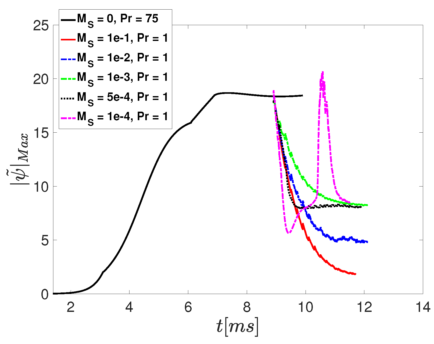
The simulations are performed by setting the initial condition, that is, q-profile, to allow for the $(2,1)$ mode to be linearly unstable. In the absence of the stochastic ZFs that is, $\delta v_S=0$, by adjusting the $Pr$ as high as 75, a non-linearly saturated state can be reached, as seen in Figure 1 where the time evolution of the $|\tilde{\psi }{|}_{max}$ is shown (see red solid line).

However, when the stochastic ZFs are included, the $(2,1)$ mode can be stabilised even at significantly lower Prandtl numbers. For example taking $M_S=5\times {10}^{-3}$ even at $Pr=10$ the mode reaches a saturated state at a lower amplitude, see the black dotted line in Figure 1.

The relationship between system stability through $Pr$ and $M_S$ (always keeping Lundquist number S fixed) shows some interesting features. For $Pr<2$, to stabilise the (2,1) mode the value of $M_S$ has to increase. For example, at very low $Pr=1.25$, the stochastic ZFs Mach number, $M_S$, has to be increased to ${10}^{-2}$ in order to avoid the blow up of the mode, see dashed-dotted blue line in Figure 1. The amplitude of the (2,1) mode in this case, is significantly reduced, and it saturates at a finite value.

In a range of $Pr>4$ and for the same value of $M_S$, the mode saturates at lower amplitudes for lower values of $Pr$, see for example green dashed dotted line vs black dotted line in Figure 1, corresponding to $Pr=4$ and $Pr=10$, respectively. We note that the simulations show that as the $Pr$ is lowered, while keeping the $M_S$ fixed, the saturation amplitude is lower. Whilst it would be reasonable to expect that the saturation level to be higher at the lower values of viscosity (i.e., lower $Pr$), the opposite is observed.

A possible explanation for this behaviour is that at high values of $Pr$, the turbulence driven small scales will be strongly dampened by the dissipative effect of the viscosity since the damping effect of viscosity scales as ${\left|k\right|}^2$. Therefore the impact of small scale driven ZFs are diminished at these high values of $Pr$. At lower values of $2<Pr<4$, this damping effect is reduced and ZFs are more efficient at stabilising the (2,1) mode.

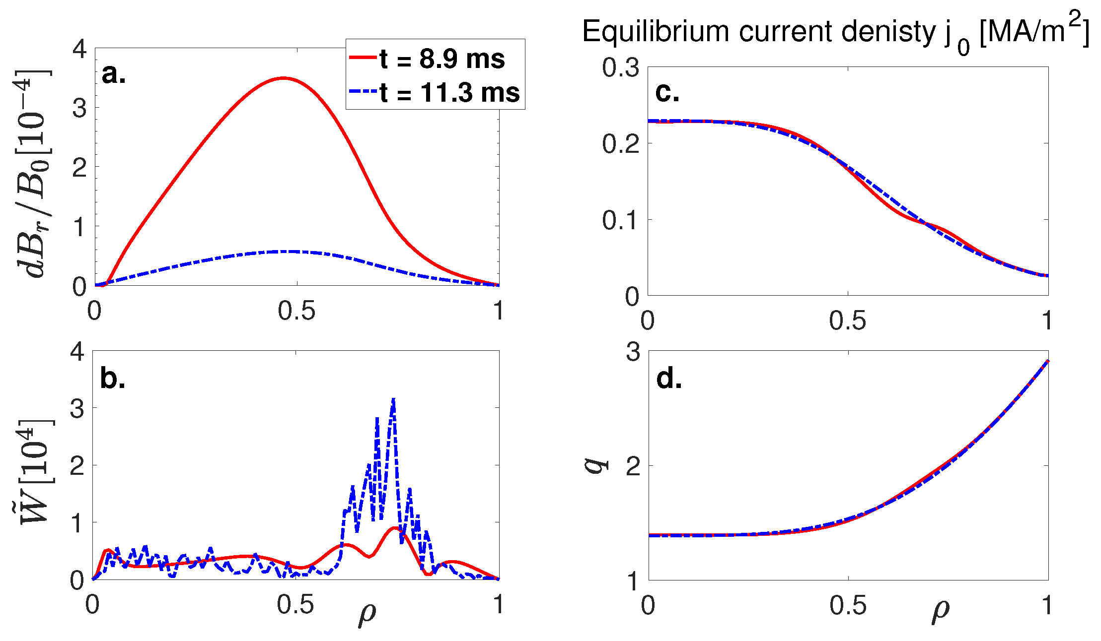
Figure 2a–d show the corresponding profiles of the $d{B}_r/B_0$, $\tilde{W}$, equilibrium current density $j_0$, and safety factor q, for the case with $Pr=1.25$. The values are compared between $t=8.9$ ms and $t=11.3$ ms, without and with the stochastic ZFs effects, respectively. As can be seen here, stochastic ZFs can result in a significant stabilisation of the (2,1) mode, comparing the red solid line to the blue dash-dotted line. In the pre ZFs state, $j_0$ shows local flattening around $q=2$ resonant surface, which is changed by the ZFs almost back to the linearly unstable original state. Thus, in effect, the ZFs are actually stabilising the (2,1) linearly unstable mode. The vorticity profile in this case shows peaks with higher amplitudes than in the absence of the stochastic ZFs model at $\rho \sim$ 0.6–0.8, corresponding to the radial location of the (2,1) mode (see blue dashed line in Figure 2b). This indicates that the ZFs promote a direct cascade in the vorticity distribution of the (2,1) mode. The free energy of the equilibrium $j_0$, is transferred through the ZFs to the high k vorticity of the mode, where viscosity is able to dissipate it, thus resulting in the lowering of the amplitude of the magnetic fluctuations.

Figure 3 illustrates the contour plots (top) and the corresponding spectra (bottom) of the current density fluctuations at the selected times. The poloidal structure of the (2,1) mode remains visible at $t=11.3$ ms. However, the amplitude is reduced significantly. This can also be seen in the spectra plots where a strong reduction of the current density fluctuation amplitude is obtained.

To determine the stability dependence of the (2,1) on the amplitude of the ZFs represented by the Mach number, $M_S$, a sensitivity scan in $(Pr,M_S)$-space was performed, while holding all other parameters fixed. The results are shown in Figure 4. The stability boundary indicates that for $2<Pr$ the minimum ZFs Mach number that is required to stabilise the (2,1) mode is $M_S\sim 5\times {10}^{-3}$, whilst for $1<Pr<2$ this level has to increase, and for example for a $Pr\sim 1$ it has to be as high as $M_S\sim 1.5\times {10}^{-2}$. In the very low viscosity regime ($Pr<2$) mode saturation requires an inverse relationship between $Pr$ and $M_S$.

In summary, by applying a simple passive stochastic ZFs model we were able to stabilise the (2,1) tearing mode at a very low kinematic viscosity represented by the Prandtl number, $Pr$ for which the mode is linearly unstable. To stabilise the (2,1) mode for a wide range of $Pr>2$, we find that the required Mach number is around $M_S=5\times {10}^{-3}$ which is of the same order as the ZFs that is expected to be generated by the small scale turbulence that is, with a ZFs velocity of the order of few $km/s$.

Note that, in principle the Stochastic ZFs should be introduced in $v0·\nabla \tilde{W}$ as well as $\frac{v_{th}{\rho }_s^{*}}{r}\{\tilde{W},\tilde{\varphi }\}$ term, but our analysis shows that for micro-turbulence relevant Alfvén Mach numbers, the impact of the stochastic ZFs from the first term are insignificant as compared to that of the second term. In the first term, the ZFs slightly advect the MHD islands back and forth in the radial direction, while they introduce significant shearing of the islands, leading to their breakup and thus stabilisation of the MHD modes through $\frac{v_{th}{\rho }_s^{*}}{r}\{\tilde{W},\tilde{\varphi }\}$ term. Therefore, we have neglected effects due to the first term.

4. Results for Semi-Stochastic Coupling Model

In order to model the dynamics involved in the interaction of the visco-resistive MHD and the turbulence, in a simplified way, we have introduced a “semi-stochastic” coupling model, where the amplitude of the stochastic ZFs is defined as $\delta v_S=M_S{v}_A\langle {\left(\tilde{j}\right)}^2+{(\tilde{W})}^2\rangle X(\rho ,t)$, with $\langle \dots \rangle$ denoting average over the flux surfaces.

Here, we expect that as the amplitude of the MHD mode increases, the amplitudes of the stochastic ZFs also increase. Note that in our model, the stochasticity properties of the stochastic variable $X(\rho ,t)$ are not changed. In this formulation, we attempt to model the MHD mode influence (via a direct cascade) on the interaction of the high k turbulence with the mode itself.

For this model, we have examined two types of MHD instabilities: (i) $(2,1)$ tearing mode and (ii) $(1,1)$ kink mode. This is done by setting the initial q and $j_0$-profiles such that the modes are linearly unstable. The time evolution of the $|\tilde{\psi }{|}_{max}$ for case (i) is shown in Figure 5. Here, we examine the effect on the MHD stabilisation for different $M_S$ at $Pr=1$.

We start from the saturated phase of the $Pr=75$, $M_S=0$ (at $t=8.9$ ms) simulation, and continue while applying the semi-stochastic coupling model, and reducing the Prandtl number to $Pr=1$ (for $t>8.9$ ms). Figure 5 shows the results of these simulations for a wide range in $M_S={10}^{-4}-{10}^{-1}$.

Our results show that a complex dynamic interaction exists between the MHD and ZFs. Initially, as $M_S$ is decreased (from ${10}^{-1}$ to ${10}^{-3}$), the stabilisation effect of the stochastic ZFs becomes less strong, and therefore, the $(2,1)$ mode saturates at higher amplitudes; compare red solid line at $M_S={10}^{-1}$ to the green dashed line at $M_S={10}^{-3}$. However, further reduction of the $M_S$ stabilises the $(2,1)$ at a faster rate; see black dotted line in Figure 5 corresponding to $M_S=5\times {10}^{-4}$.

Decreasing the $M_S$ to ${10}^{-4}$ increases this initial decay rate even further. However, after reaching a threshold level, it transiently rises to a higher amplitude before eventually saturating to the same amplitude as with $M_S={10}^{-3}$; see pink dashed-dotted line in Figure 5 corresponding to $M_S={10}^{-4}$. A possible reason for this observation is that as the amplitude of the initial seed of ZFs becomes weaker that is, lowering of the $M_S$, the (2,1) mode grows rapidly since at the same time we have significantly reduced the stabilisation effect of $Pr$. As the mode’s growth becomes more rapid, the increase in the amplitude of the seeded ZFs grows (due to the $\langle {\left(\tilde{j}\right)}^2+{(\tilde{W})}^2\rangle$ factor). Therefore, the stabilisation effect of the ZFs becomes stronger and stronger increasing the damping rate of the $|\tilde{\psi }{|}_{max}$, as observed in Figure 5 black dotted line compared to green dashed line.

Consider the difference between the black dotted line ($M_S=5\times {10}^{-4}$) and the pink dashed-dotted line ($M_S={10}^{-4}$), in Figure 5. The rapid transient growth of the mode amplitude due to the significantly lower $M_S$ results in a very large rise of the non-linear factor $\langle {\left(\tilde{j}\right)}^2+{(\tilde{W})}^2\rangle$. As expected, the mode drives the ZFs strongly leading to even faster damping. This results in the pink dashed-dotted line reaching a minimum at about $t\sim 9.2$ ms well bellow the black dotted line, in Figure 5. On the other hand, if the mode decays too rapidly to very low levels, the ZFs amplitude decays with it and so does its stabilisation impact on the (2,1) mode. As soon as the ZFs stability effect disappears, the non-linear growth of the mode rapidly results in an overshoot (see pink dashed-dotted line in Figure 5 at $t=10.4$ ms where the mode has reached reaching its maximum at $t\sim 10.4$ ms well above the saturation level of the black dotted line). At this point, the ZFs become large enough to suppress the non-linear growth and stabilise the system to reach a new saturated state which is essentially similar to the previous cases. For a range of initial ZFs seeds with $M_S={10}^{-4}-{10}^{-3}$, we observe a non-linear self-organziation interplay between ZFs, $(2,1)$ and its related low (m,n) spectrum that saturates to a similar final state.

Figure 6a–d show a comparison of the profiles of the $d{B}_r/B_0$, $\tilde{W}$, equilibrium current density $j_0$, and safety factor q between $t=8.9$ ms and $t=11.7$ ms, without and with the stochastic ZFs, respectively. The equilibrium current profile $j_0$ in the final saturated state, is almost back to its original linearly unstable profile, in the case where $M_S={10}^{-1}$ (see Figure 6c). However, the saturated mode amplitude is low $d{B}_r/B_0\sim {10}^{-4}$, thus, the overall ZFs Mach number is of the order of ${10}^{-3}$.

The vorticity profile in this case shows two distinct peaks with significantly higher amplitudes than in the absence of the stochastic ZFs at $\rho \sim 0.65$ and $\rho \sim 0.75$ (see blue dashed line in Figure 6b). The impact of this strong shear in the vorticity is observed on the sheared poloidal structure of the current density fluctuations with two peaks developed at $m=2$ surface, see the contour plots shown in Figure 7 (left) and the corresponding spectra plots in Figure 7 (right). Furthermore, a low amplitude $m=5,n=4$ mode is found to be active in the plasma core.

In case (ii) for the $(1,1)$ mode we start with the Prandtl number of $Pr=30$ (as was reported in Reference [7]), and after reaching a non-linear saturated state at time $t=2.64$ ms, we apply the stochastic ZFs model as described above whilst reducing the Prandtl number to $Pr=1$. As can be seen in Figure 8, for very small values of the $M_S=5\times {10}^{-5}$ (pink dashed-dotted line), initially the $(1,1)$ mode grows strongly due to the lower Prandtl number, however as its amplitude increases, so does the amplitude of the stochastic ZFs, which eventually leads to stabilisation and saturation of the mode. We note that during this mode evolution, the equilibrium state also changes ($d{j}_0/dr$) due to the non-linear effects of the mode on itself, the so-called profile-mode interaction [7]. After that the mode fluctuates around its original saturated level in the absence of the stochastic ZFs with $Pr=30$. By increasing $M_S$, a new saturated state can be reached but at a significantly lower amplitude (see for example, red solid line in Figure 8 for $M_S={10}^{-1}$). This dynamic behaviour is closely related to the dynamics that we described in the (2,1) case where the equilibrium current profile $j_0$ in the final saturated state, is almost back to its original linearly unstable profile (see Figure 9c). However, the saturated mode amplitude is low $d{B}_r/B_0\sim {10}^{-5}$, thus, the overall ZFs Mach number is agin of the order of ${10}^{-3}$.

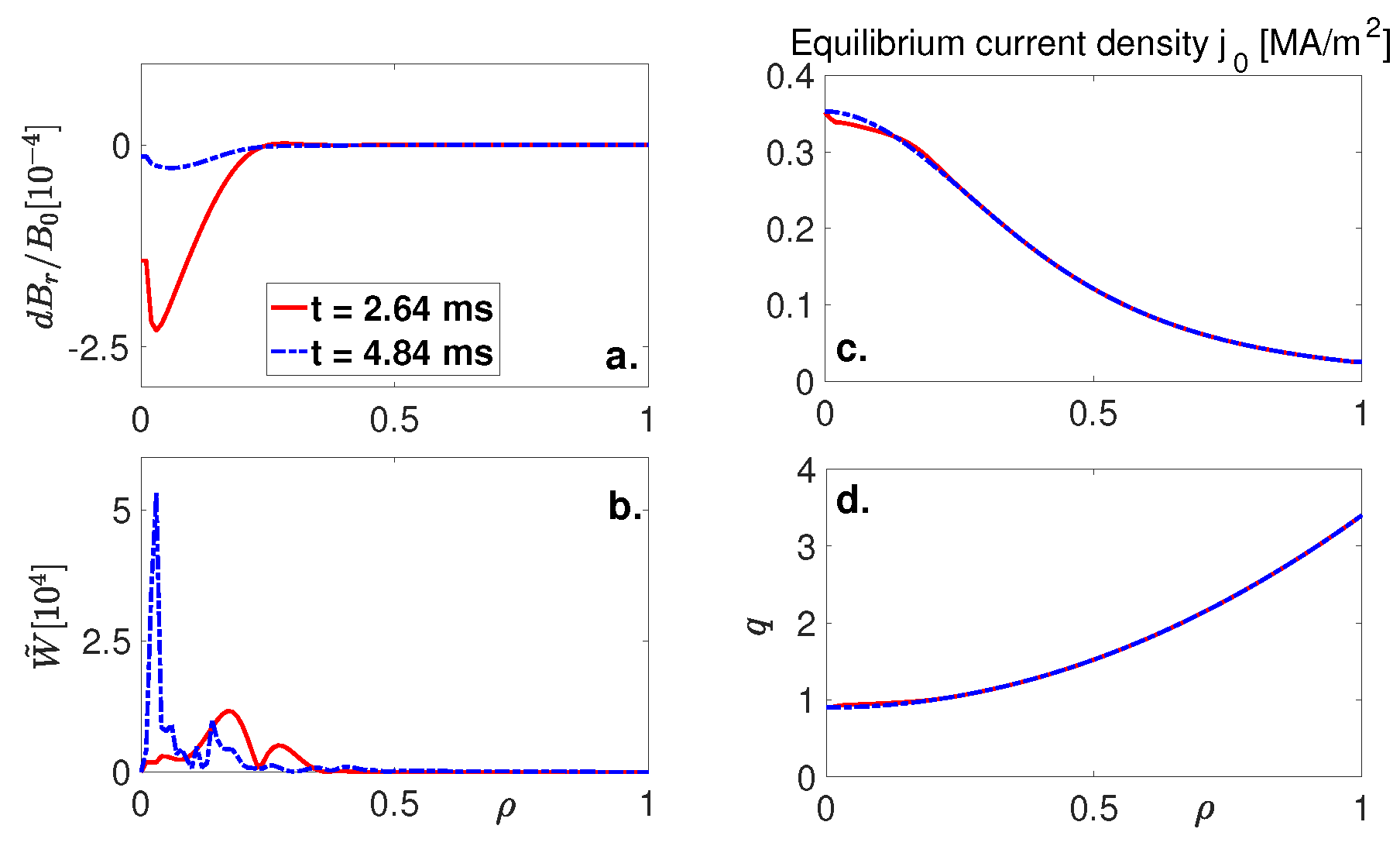
Figure 9a–d show a comparison of the profiles of the $d{B}_r/B_0$, $\tilde{W}$, equilibrium current density $j_0$, and the safety factor q at $t=2.64$ ms and $t=4.64$ ms, without and with the stochastic ZFs effects at $M_S={10}^{-1}$, respectively. As can be seen here, addition of the stochastic ZFs results in a significant stabilisation of the $(1,1)$ mode, comparing the red solid line to the blue dash-dotted line in Figure 9a. The distortion of the equilibrium current density due to the $(1,1)$ mode is strongly reduced as the model is applied. The vorticity profile in this case shows a more localised peak with larger amplitude at $\rho \sim 0.15$ (see blue dashed line in Figure 9b). The impact of this strong shear in the vorticity is observed on the poloidal structure of the current density fluctuations at $m=1$ surface, see the contour plots shown in Figure 10 (Top) and the corresponding spectra plots in Figure 10 (Bottom).

In summary, by applying a semi-stochastic ZFs model we were able to stabilise the $(2,1)$ tearing mode and the $(1,1)$ kink mode at a very low kinematic viscosity represented by the Prandtl number, $Pr$ for which the modes are linearly unstable. The main difference here with that of the simple stochastic model discussed in the previous section is that, the dynamic stabilisation is more effective even at lower $M_S$ and after an initial oscillation the saturation levels for different values of $M_S$ are similar due to the interaction between MHD and turbinate.

5. Conclusions

A model is developed to simulate micro-scale turbulence driven ZFs, and their impact on the MHD tearing and kink modes is examined. The model is based on a stochastic representation of the micro-scale ZFs with a given Mach number, $M_S$. Two approaches were considered (i) passive stochastic model where the ZF’s amplitudes are independent of the MHD mode amplitude, and (ii) the semi-stochastic model where the amplitudes of the ZFs have a dependence on the amplitude of the MHD mode itself. We have purposely kept the resistive diffusivity ($c^2\eta /4\pi$), and the kinematic viscosity ($\nu$) as given functions of $\rho$, and during the time evolution of the system, in order to explore the advective effects of the stochastic ZFs on the vorticity equation. We recognise that in principle, the small-scale turbulence can also modify both of these transport properties for example as it is done in previous two-fluid simulations with CUTIE (Thyagaraja et al. [48]). In neutral fluid dynamics, it has long been recognised (since the time of Prandtl), that turbulence modifies momentum and energy transport properties of the fluid significantly above their Laminar/molecular values.

The results for the approach (i) show that the stochastic ZFs can significantly stabilise the (2,1) mode even at very low kinematic viscosity, $Pr$, where the mode is linearly unstable. For very low levels of $Pr<2$ the stochastic ZFs amplitude, described by its Mach number $M_S$ has to increase, in order for stabilisation to be effective. However, for $Pr>2$, and at similar values of $M_S$, we find that lower values of $Pr$ lead to lower saturation levels of the MHD mode. This is understood to be the result of stronger dissipation of the ZFs at higher $Pr$, which reduces their stabilisation effect on the MHD mode.

In approach (ii) we observe a more complex interaction between the ZFs and the MHD modes (both (2,1) and (1,1) modes), where by decreasing the amplitude of the initial seeded ZFs, that is, $M_S$, the damping rate of the MHD modes actually increases even at linearly unstable $Pr$ levels. This dynamic behaviour is understood to be a result of a predator-prey type of dynamical stabilisation where the initial seeded ZFs are too small to damp the MHD mode. However since the stabilisation effect of the viscosity ($Pr$) has also diminished in these cases, the mode amplitude shoots up. As the amplitude of ZFs are dependent on the energy of the mode, they will grow very fast and back-react on the mode leading to a faster decay rate. For $M_S$ values below a threshold, the fast decay of the MHD also kills the ZFs, and hence, it starts to grow again. As the ZFs grow with the mode, at some point they reach a level that can stabilise the MHD mode once more. In our examples, we have not observed any repetition of this cycle, and after this initial interaction between the ZFs and MHD mode, they saturate to an invariant final state (for ${10}^{-5}<M_S<{10}^{-3}$). The equilibrium current density profile in this final state is close to the initial linearly unstable profile. We note however, that the possibility of a “Hopf bifurcation” with periodic waxing and wining of the mode and turbulence is not ruled out and may occur for different choices of parameters.

Our results, therefore, indicate a possible mechanism for stabilisation of the MHD modes via small-scale perturbations in poloidal flow, simulating the turbulence driven ZFs. Generating small-scale perturbations in the vicinity of the MHD modes, without the need for high spatial accuracy, in principle can be achieved by means of Radio Frequency waves (RF). As it is already demonstrated, in fusion plasmas application of RF heating has a stabilisation impact on the core MHD modes such as Sawteeth [17,18]. Here, we propose that by activation of micro-turbulence as a result of RF heating, and thus increase in temperature gradient, the associated sheared ZFs can be expected to dampen the MHD. This mechanism is shown here in a very simplified form, and further studies on its dynamic is the subject of our future work.

References

- Marshall, P.; Rosenbluth, N.; Dagazian, R.Y. Nonlinear properties of the internal m = 1 kink instability in the cylindrical tokamak. Phys. Fluids 1973, 16, 1894–1902. [Google Scholar]
- Goeler, S.V.; Stodiek, W.; Sauthoff, N. Studies of Internal Disruptions and m = 1 Oscillations in Tokamak Discharges with Soft–X-Ray Techniques. Phys. Rev. Lett. 1974, 33, 1201–1203. [Google Scholar] [CrossRef]
- Kadomtsev, B.B. Disruptive instability in Tokamaks. Fiz. Plazmy 1975, 1, 710–715, reprinted in Sov. J. Plasma Phys. 1975, 1, 389–391. [Google Scholar]
- Thyagaraja, A.; Haas, F.A. Asymptotic theory of the nonlinearly saturated m = 1 mode in tokamaks with q0 < 1. Phys. of Plasmas 1991, 3, 580. [Google Scholar]
- Porcelli, F.; Boucher, D.; Rosenbluth, M.N. Model for the sawtooth period and amplitude. Plasma Phys. Controlled Fusion 1996, 38, 2163–2186. [Google Scholar] [CrossRef]
- Monticello, D.A.; Park, W.; Izzo, R.; McGuire, K. A review of calculations of the resistive internal m = 1 mode in Tokamaks. Comput. Phys. Commun. 1986, 43, 57–67. [Google Scholar] [CrossRef]
- Mendonca, J.; Chandra, D.; Sen, A.; Thyagaraja, A. Visco-resistive MHD study of internal kink (m = 1) modes. Phys. Plasmas 2018, 25, 022504. [Google Scholar] [CrossRef]
- Cao, K.; Wang, X. The theory of early nonlinear stage of m = 1 instability with locally flattened q-profile. Matter and Radiation at Extremes 2018, 3, 243. [Google Scholar] [CrossRef] [Green Version]
- Wilson, H.; Connor, J.; Hastie, R.; Hegna, C. Threshold for neoclassical magnetic islands in a low collision frequency tokamak. Phys. of Plasmas 1996, 3, 248. [Google Scholar] [CrossRef]
- Haye, R.L.; Gunter, S.; Humphreys, D.; Lohr, J.; Luce, T.; Maraschek, M.; Petty, C.; Prater, R.; Scoville, J.; Strait, E. Control of neoclassical tearing modes in DIII-D. Phys. of Plasmas 2002, 9, 2051. [Google Scholar] [CrossRef] [Green Version]
- Smolyakov, A.I. Nonlinear evolution of tearing modes in inhomogeneous plasmas. Plasma Phys. Controlled Fusion 1993, 35, 657. [Google Scholar] [CrossRef]
- Hegna, C. The physics of neoclassical magnetohydrodynamic tearing modes. Phys. Plasmas 1998, 5, 1767. [Google Scholar] [CrossRef]
- Chang, Z.; Callen, J.; Fredrickson, E.; Budny, R.; Hegna, C.; Mcguire, K.; Zarnstorff, M. Observation of nonlinear neoclassical pressure-gradient-driven tearing modes in TFTR. Phys. Rev. Lett. 1995, 74, 4663. [Google Scholar] [CrossRef]
- Carrera, R.; Hazeltime, R.; Kotschenreuther, M. Island bootstrap current modification of the nonlinear dynamics of the tearing mode. Phys. Fluids 1986, 29, 899. [Google Scholar] [CrossRef]
- McDevitt, J.; Diamond, P.H. Multiscale interaction of a tearing mode with drift wave turbulence: A minimal self-consistent model. Phys. Plasmas 2006, 13, 032302. [Google Scholar] [CrossRef] [Green Version]
- Chandra, D.; Thyagaraja, A.; Sen, A.; Ham, C.; Hender, T.; Hastie, R.; Connor, J.; Kaw, P.; Mendonca, J. Modelling and analytic studies of sheared flow effects on tearing modes. Nucl. Fusion 2015, 55, 053016. [Google Scholar] [CrossRef]
- Lerche, E.; Lennholm, M.; Carvalho, I.S.; Dumortier, P.; Durodie, F.; Eester, D.V.; Graves, J.; Jacquet, P.; Murari, A. JET Contributors, Sawtooth pacing with on-axis ICRH modulation in JET-ILW. Nucl. Fusion 2017, 57, 036027. [Google Scholar] [CrossRef] [Green Version]
- Campbell, D.J.; Start, D.F.H.; Wesson, J.A.; Bartlett, C.V.; Bhatnagar, V.P.; Bures, M.; Cordey, J.G.; Cottrell, G.A.; Dupperex, P.A.; Edwards, A.W.; et al. Stabilization of sawteeth with additional heating in the JET tokamak. Phys. Rev. Lett. 1988, 60, 2148. [Google Scholar] [CrossRef]
- McClements, K.G.; Dendy, R.O.; Hastie, R.J.; Martin, T.J. Modeling of sawtooth destabilization during radio?frequency heating experiments in tokamak plasmas. Phys. Plasmas 1996, 3, 2994. [Google Scholar] [CrossRef] [Green Version]
- Yang, X.; Wang, S.; Yang, W. Stabilization of tearing modes by oscillating the resonant surface. Phys. of Plasmas 2012, 19, 072503. [Google Scholar] [CrossRef]
- Mao, J.; Phillips, P.E.; Gentle, K.W.; Zhao, J.; Zhang, X.; Luo, J.; Li, J.; Zhang, S.; Gao, X.; Li, Y.; et al. Modulated toroidal current suppression of MHD activity on the HT-7 superconducting tokamak. Nucl. Fusion 2001, 41, 1645. [Google Scholar] [CrossRef]
- de Vries, P.C.; Johnson, M.F.; Segui, I. JET EFDA Contributors. Statistical analysis of disruptions in JET. Nucl. Fusion 2009, 49, 055011. [Google Scholar] [CrossRef]
- de Vries, P.C.; Baruzzo, M.; Hogeweij, G.M.D.; Jachmich, S.; Joffrin, E.; Lomas, P.J.; Matthews, G.F.; Murari, A.; Nunes, I.; Pütterich, T.; et al. The influence of an ITER-like wall on disruptions at JET. Phys. Plasmas 2014, 21, 056101. [Google Scholar] [CrossRef]
- Lehnen, M.; Arnoux, G.; Brezinsek, S.; Flanagan, J.; Gerasimov, S.N.; Hartmann, N.; Hender, T.C.; Huber, A.; Jachmich, S.; Kiptily, V. Impact and mitigation of disruptions with the ITER-like wall in JET. Nucl. Fusion 2013, 53, 093007. [Google Scholar] [CrossRef]
- Ishizawa, A.; Kishimoto, Y.; Nakamura, Y. Multi-scale interactions between turbulence and magnetic islands and parity mixtur-a review. Plasma Phys. Control. Fusion 2019, 61, 054006. [Google Scholar] [CrossRef]
- Ishizawa, A.; Maeyama, S.; Watanabe, T.; Sugama, H.; Nakajima, N. Electromagnetic gyrokinetic simulation of turbulence in torus plasmas. J. Plasma Phys. 2015, 81, 435810203. [Google Scholar] [CrossRef]
- Coppi, B.; Spight, C. Ion-mixing mode and model for density rise in confined plasmas. Phys. Rev. Lett. 1977, 41, 551. [Google Scholar] [CrossRef]
- Kadomtsev, B.B.; Pogutse, O.P. Trapped particles in toroidal magnetic systems. Nucl. Fusion 1971, 11, 67. [Google Scholar] [CrossRef]
- Dorland, W.; Jenko, F.; Kotschenreuther, M.; Rogers, B.N. Electron temperature gradient turbulence. Phys. Rev. Lett. 2000, 85, 5579. [Google Scholar] [CrossRef]
- Pueschel, M.J.; Kammerer, M.; Jenko, F. Gyrokinetic turbulence simulations at high plasma beta. Phys. Plasmas 2008, 15, 102310. [Google Scholar] [CrossRef] [Green Version]
- Doerk, H.; Jenko, F.; Pueschel, M.J.; Hatch, D.R. Gyrokinetic microtearing turbulence. Phys. Rev. Lett. 2011, 106, 155003. [Google Scholar] [CrossRef] [PubMed] [Green Version]
- Guttenfelder, W.; Candy, J.; Kaye, S.M.; Nevins, W.M.; Wang, E.; Zhang, J.; Bell, R.E.; Crocker, N.A.; Hammett, G.W.; LeBlanc, B.P.; et al. Scaling of linear microtearing stability for a high collisionality National Spherical Torus Experiment discharge. Phys. Plasmas 2012, 19, 022506. [Google Scholar] [CrossRef]
- Moradi, S.; Pusztai, I.; Guttenfelder, W.; Fülöp, T.; Mollén, A. Microtearing modes in spherical and conventional tokamaks. Nucl. Fusion 2013, 53, 063025. [Google Scholar] [CrossRef] [Green Version]
- Li, J.; Kishimoto, Y. Small-scale dynamo action in multi-scale magnetohydrodynamic and micro-turbulence. Phys. Plasmas 2012, 19, 030705. [Google Scholar] [CrossRef] [Green Version]
- Ishizawa, A.; Waelbroeck, F.L. Magnetic island evolution in the presence of ion-temperature gradient-driven turbulence. Phys. of Plasmas 2013, 20, 122301. [Google Scholar] [CrossRef]
- Sun, P.J.; Li, Y.D.; Ren, Y.; Zhang, X.D.; Wu, G.J.; Xu, L.Q.; Chen, R.; Li, Q.; Zhao, H.L.; Zhang, J.Z.; et al. The EAST Team, Experimental identification of nonlinear coupling between (intermediate, small)-scale microturbulence and an MHD mode in the core of a superconducting tokamak. Nucl. Fusion 2018, 58, 016003. [Google Scholar] [CrossRef] [Green Version]
- Ishizawa, A.; Nakajima, N. Excitation of macromagnetohydrodynamic mode due to multiscale interaction in a quasi-steady equilibrium formed by a balance between microturbulence and zonal flow. Phys. Plasmas 2007, 14, 040702. [Google Scholar] [CrossRef] [Green Version]
- Li, J.; Kishimoto, Y.; Kouduki, Y.; Wang, Z.X.; Janvier, M. Finite frequency zonal flows in multi-scale plasma turbulence including resistive MHD and drift wave instabilities. Nucl. Fusion 2009, 49, 095007. [Google Scholar] [CrossRef]
- Poli, E.; Bottino, A.; Peeters, A.G. Behaviour of turbulent transport in the vicinity of a magnetic island. Nucl. Fusion 2009, 49, 075010. [Google Scholar] [CrossRef] [Green Version]
- Hariri, F.; Hill, P.; Ottaviani, M.; Sarazin, Y. Plasma turbulence simulations with X-points using the flux-coordinate independent approach. Plasma Phys. Control. Fusion 2015, 57, 054001. [Google Scholar] [CrossRef] [Green Version]
- Hornsby, W.A.; Migliano, P.; Buchholz, R.; Zarzoso, D.; Casson, F.J.; Poli, E.; Peeters, A.G. On seed island generation and the non-linear self-consistent interaction of the tearing mode with electromagnetic gyro-kinetic turbulence. Plasma Phys. Control. Fusion 2015, 57, 054018. [Google Scholar] [CrossRef] [Green Version]
- Bardoczi, L.; Carter, T.A.; Haye, R.J.L.; Rhodes, T.L.; McKee, G.R. Impact of neoclassical tearing mode-turbulence multi-scale interaction in global confinement degradation and magnetic island stability. Phys. Plasmas 2017, 24, 122503. [Google Scholar] [CrossRef]
- Bardoczi, L.; Rhodes, T.L.; Carter, T.A.; Navarro, A.B.; Peebles, W.A.; Jenko, F.; McKee, G.R. Modulation of core turbulent density fluctuations by large-scale neoclassical tearing mode islands in the DIII-D tokamak. Phys. Rev. Lett. 2016, 116, 215001. [Google Scholar] [CrossRef] [Green Version]
- Thyagaraja, A.; Hazeltine, R.D.; Aydemir, A.Y. Stabilization of the m = 1 tearing mode by resonance detuning. Phys. Fluids B Plasma Phys. 1992, 4, 2733. [Google Scholar] [CrossRef]
- Thyagaraja, A.; Haas, F.A. Two novel applications of bootstrap currents: Snakes and jitter stabilization. Phys. Fluids B Plasma Phys. 1993, 5, 3252. [Google Scholar] [CrossRef] [Green Version]
- Krommes, J.A. The roles of shear and cross-correlations on the fluctuation levels in simple stochastic models. Phys. Plasmas 2000, 7, 1148. [Google Scholar] [CrossRef]
- De Vries, P.C.; Donne, A.J.H.; Heijnen, S.H.; Hugenholtz, C.A.J.; Kramer-Flecken, A.; Schuller, F.C.; Waidmann, G. Density profile peaking inside m/n = 2/1 magnetic islands in TEXTOR-94. Nucl. Fusion 1997, 37, 1641. [Google Scholar] [CrossRef]
- Thyagaraja, A.; Valovič, M.; Knight, P.J. Global two-fluid turbulence simulations of LH transitions and edge localized mode dynamics in the COMPASS-D tokamak. Phys. Plasmas 2010, 17, 042507. [Google Scholar] [CrossRef] [Green Version]
- Yu, Q.; Gunter, S.; Lackner, K. Formation of plasmoids during sawtooth crashes. Nucl. Fusion 2014, 54, 072005. [Google Scholar] [CrossRef] [Green Version]
- Diamond, P.H.; Itoh, S.; Itoh, K.; Hahm, T.S. Zonal flows in plasm-a review. Plasma Phys. Control. Fusion 2005, 47, R35. [Google Scholar] [CrossRef]
Figure 1.
Time evolutions of the for (2,1) mode for various levels of Prandtl number , and the amplitude of the stochastic Zonal Flows (ZFs), .
Figure 2.
The profiles of the (a), (b), equilibrium current density (c), and safety factor q (d) for the (2,1) mode case, at time ms corresponding to (red solid lines), and ms corresponding to (blue dotted lines).
Figure 3.
Top: The contour plots of the current density fluctuations at ms corresponding to the saturated level with (left), and at ms with (right). Bottom: The corresponding spectra of the current density fluctuations as functions of and poloidal mode number m, at ms (left) and ms (right).
Figure 4.
The stability boundary for (2,1) mode as functions of Prandtl number, , and the amplitude of the stochastic ZFs, .
Figure 5.
Time evolutions of the for (2,1) mode for (black solid line) and (all other lines), for various levels of the amplitude of the stochastic ZFs, .
Figure 6.
The profiles of the (a), (b), equilibrium current density (c), and safety factor q (d) for the mode case, at time ms corresponding to (red solid lines), and ms corresponding to (blue dotted lines).
Figure 7.
Left: The contour plots of the current density fluctuations at ms corresponding to the saturated level with . Right: The corresponding spectra of the current density fluctuations as functions of and poloidal mode number m.
Figure 8.
Time evolutions of the for (1,1) mode for (black solid line) and (all other lines) for various levels the Mach number of the stochastic ZFs, .
Figure 9.
Figure 10.
© 2020 by the authors. Licensee MDPI, Basel, Switzerland. This article is an open access article distributed under the terms and conditions of the Creative Commons Attribution (CC BY) license (http://creativecommons.org/licenses/by/4.0/).
Share and Cite
MDPI and ACS Style
Moradi, S.; Thyagaraja, A. Impact of Micro-Scale Stochastic Zonal Flows on the Macro-Scale Visco-Resistive Magnetohydrodynamic Modes. Mathematics 2020, 8, 443. https://doi.org/10.3390/math8030443
AMA Style
Moradi S, Thyagaraja A. Impact of Micro-Scale Stochastic Zonal Flows on the Macro-Scale Visco-Resistive Magnetohydrodynamic Modes. Mathematics. 2020; 8(3):443. https://doi.org/10.3390/math8030443
Chicago/Turabian StyleMoradi, Sara, and Anantanarayanan Thyagaraja. 2020. "Impact of Micro-Scale Stochastic Zonal Flows on the Macro-Scale Visco-Resistive Magnetohydrodynamic Modes" Mathematics 8, no. 3: 443. https://doi.org/10.3390/math8030443
Note that from the first issue of 2016, this journal uses article numbers instead of page numbers. See further details here.