QMwebJS—An Open Source Software Tool to Visualize and Share Time-Evolving Three-Dimensional Wavefunctions

Abstract

Numerical simulation experiments are of great importance for research and education in Physics. They can be greatly aided by proper graphical representations, especially for spatio-temporal dynamics. In this contribution, we describe and provide a novel Javascript-based library and cloud microservice—QMwebJS—for the visualization of the temporal evolution of three-dimensional distributions. It is an easy to use, web-based library for creating, editing, and exporting 3D models based on the particle sampling method. Accessible from any standard browser, it does not require downloads or installations. Users can directly share their work with other students, teachers or researchers by keeping their models in the cloud and allowing for interactive viewing of the spatio-temporal solutions. This software tool was developed to support quantum mechanics teaching at an undergraduate level by plotting the spatial probability density distribution given by the wavefunction, but it can be useful in different contexts including the study of nonlinear waves.

1. Introduction

In the last decades, the rapid development of hardware and software has opened many new avenues and modified the workflows of scientific research. The same is true for technical education in different disciplines, and in particular in Physics. The concept of a “virtual” or “in-silico” “laboratory” has been developed, that is, the utilization of computers to generate interactive environments to perform simulated experiments and analyze their results. It has been argued that combining physical and virtual investigations can strengthen science learning and help to better engage and motivate students in scientific experiences [1]. In particular, adequate visualizations play a critical role in enhancing science and engineering learning [2]. Graphical displays are an important tool because addressing a given concept from the point of view of multiple representations brings unique benefits for students [3].

Information and communication technologies have facilitated the expansion of distance learning and both virtual laboratories and interactive computer experiments have been fruitful in this context [4]. Being affordable and easily accessible to students, such systems can also support inquiry-based learning [5]. Computer-assisted tools can also be more advantageous than experiments in some cases, for instance when they allow faster manipulation than actual physical devices [6]. Such systems can also make scientific inquiry more tangible and attractive for students. For undergraduate level quantum mechanics, new computer graphics tools could compensate for the inherent lack of experiment-assisted visualizations, thereby serving to clarify conceptual difficulties and misconceptions of spatial wavefunctions [7]. Studies have shown how modules that simulate and display the evolution of the Schrödinger equation can be successfully integrated in introductory Quantum Physics courses [8]. In this context, a recent study [9] emphasizes the fundamental importance of understanding the time evolution of quantum systems and discusses the serious difficulties that students often encounter.

Here, we describe an open-source, web-based software tool (implemented as a client-side javascript library, called QMwebJS) for interactive three-dimensional (3D) visualization of the evolution of quantum wavefunctions obtained from numerical simulations. This tool is an example of how modern web technology can be leveraged for making complex visualizations of scientific and engineering simulations, while being both easy to use and more engaging for students. The wavefunction at time t is represented as a collection of points, sampled from the probability amplitude, ${|\mathsf{\Psi }(t,\mathbf{x})|}^2$. Since the wavefunction is represented as a cloud of points, as opposed to more traditional isocontour plots, all the wave-like dynamics can be seen simultaneously throughout the entire wavefunction volume. In this way, a more accurate representation of the wavefunction and computer simulations of the Schrödinger equation can provide students with remarkable insight into a large spectrum of quantum systems. These graphical representations can also be valuable for interpreting new phenomena and provide a means to more easily communicate such results to other scientists.

Computational scientists often use computer languages or packages, designed specifically for numerical simulations, that are equipped with graphics libraries for producing 3D plots (and videos) of their simulation results. Indeed, many commercial mathematical software packages include 3D display functions and have been widely used for educational purposes (see e.g., Reference [10]). As just mentioned, often such displays of the wavefunction are provided as isocontour approximations, which do not fully capture the intricate dynamics throughout the full 3D volume. Also, when sharing results with other scientists, careful selection and special setup is required to portray the most relevant subset of images. Thus, the present practice of communicating the results of numerical simulations is fraught with two fundamental problems: (1) the common representation of isosurfaces is not entirely adequate in all situations; and (2) sharing the results in video/image still does not allow other teachers, researchers, students to interactively explore the full solutions. While we treat specifically the study of the Schrödinger equation, these same issues are also applicable to other similar systems.

The QMwebJS tool, which can be used within a cloud microservice, solves these two problems. First, it provides online editing/rendering of 3D wavefunction with Monte Carlo sampling and particle visualization, reported originally with Blender3D [11]. With the help of WebGL primitives, the sampled wavefunction amplitude is represented as 3D objects (ico-spheres), that we call particles. Next, when provided as a web-based cloud service, 3D models can be created, exported, and shared with other users in order to interactively explore the results directly within a web browser, without requiring additional software installation. In this way, a user would access the web service, open the simulation results (supplied as matrices in a specified format), and use the client-browser to execute the visualization locally. Once uploaded to the browser, the 3D model is immediately instantiated, which can then be edited by changing several visual parameters (lighting, texture, color, etc.). Results of the visualization can be saved as images, videos, or exported as 3D models, which can be subsequently viewed in standard 3D viewer software, or once again in the browser using QMwebJS.

The QMwebJS javascript library fulfills the following design objectives:

• Accessible: the solution is cross-platform, since it uses standard WebGL enabled browser technology (e.g., Mozilla, Chrome, Opera), not requiring any installation.
• Easy to use: the interface is intuitive, with functionality reduced to essentials; this counters other software tools such as Blender or ParaView, that have a wider application domain, but require considerable knowledge to use.
• Efficient: the javascript app, QMwebJS, uses WebGL with the Javascript Framework Threejs; these are optimized libraries that minimize graphic latency by using features of the host GPU.
• Adaptable: QMwebJS can be used to customize 3D models to achieve the desired visualization; this is done in the real-time editor with functions for setting the 3D objects, the scale, color, and lighting effects.
• Transportable: Whether used as a stand-alone library, or used through the online platform, models can be downloaded and shared online with other researchers; models of the temporal dynamics of a simulation can be loaded and explored interactively directly in the web browser (with QMwebJS) or in any standard 3D viewer.

Even while this software was developed with the specific intention of wavefunction visualization in an educational context, it can also be used to represent any three-dimensional distribution function and therefore it might find application in many different frameworks. In particular, we believe it has potential uses for displaying research results of 3D nonlinear waves that are being actively studied in different branches of Physics, including optics, cold atoms, or cosmology.

This paper is structured as follows. Section 2 explains the details of QMwebJS; after briefly reviewing similar software, it presents the architecture, methods and algorithms on which the library is based. It is the core of the contribution but it can be skipped by the reader solely interested in the utilization of the educational tool and not in its underlying implementation details. Section 4 describes the particularities of the visualization environment and discusses its performance in terms of rendering time and memory needs. Section 5 discusses possible educational strategies and provides several examples that could be pertinent for an undergraduate Quantum Mechanics course. Section 6 presents a brief summary of results. Finally, we provide Supplementary Materials that describes the software usage and requirements of input data formats as well as a step-by-step guide for getting started with examples. A fully functional online version of QMwebJS is provided at http://www.parvis3d.org.es/. This site provides live examples provided in this paper, as well as links to download both the source code and simulation code examples. Other researchers could use our online version of QMwebJS or install the software on their own machines to produce visualizations with their own data.

2. Background

2.1. Particle Sampling for 3D Visualization

Achieving an effective visualization display of different scientific sets of data is far from a trivial problem, see Reference [12,13,14] for enlightening discussions. A useful 3D visual representation, particularly for spatiotemporal probability distributions that solve the Schrödinger equation, utilises a particle sampling method recently described [11], similar to some representations of fluid flows [15]. Briefly, ${|\mathsf{\Psi }|}^2$ is represented by a collection of 3D primitive objects (e.g., polygon-spheres, icospheres) that we call particles. They are positioned at randomly sampled points drawn from the probability density. For temporal simulations, sampling of ${|\mathsf{\Psi }|}^2$ is done for all time points. In this way, the density is directly observed for all points in the 3D volume. Interior details of the wavefunction can be observed at all times as it evolves over time, revealing simultaneous details not accessible with other display representations, such as isosurfaces.

Creating a visually satisfying 3D representation consisting of a large set of points in space requires memory efficient libraries. While this 3D editor is a highly flexible platform, it can be overpowering for the present task since its focus is towards full-featured cinemagraphic level animations. As such, we developed QMwebJS, a cross-platform web-based editor environment, as a more practical and easier solution. Another advantage is that software installation is not necessary since it only requires a modern web browser.

A useful feature of our previous approach [11] was the ability to export interactive 3D models in order to share simulation solutions. For a single instance in time, this solution is useful, however extending this to multiple models along the simulation timeline presented significant practical problems. In particular: (1) the exported models can be large (>50–200 MB) making uploads and latency a problem; and (2) evolving the simulation in time is done by switching consecutive 3D models in and out of memory, also suffering from considerable latency.

The QMwebJS solves these problems since all models of the timeline are stored and edited in the web browser (i.e., on the host computer, or the client-side). QMWebJS relies on two web-based graphics libraries: WegGL (functions implementing standard OpenGL graphics, but for web) and Threejs (extending WebGL with higher level functional event handling). However, these libraries are served through the petition of the HTML document, and the end user does not need to install additional libraries or modules other than use a modern web browser.

2.2. Background Literature on Web Based Visualization

Visualizations and 3D models are traditionally made using desktop software available commercially (e.g., 3DS Max, Maya, Catia) or as open source (e.g., Blender, ParaView). Given the end goal of these tools (i.e., cinematography or game development), they are specialized software tools targeted for high-end desktop rendering performance, artistic creativity, and complex cinematographic production pipelines.

For most cases, and in particular for educational purposes, an easy-to-use web/cloud based solution is more advantageous, not requiring software installation/learning. Several scientific visualization projects based on cloud solutions have been reported recently in the literature. These tools allow sharing, editing, and storing of scientific visualizations through the web. Reference [16] presents a microservice based architecture that uses cloud computing on Amazon Web Services (AWS) for server computation that enable interactive visualizations embedded in web. Web based generated visualization of high dimensional data with the tool SPOT was recently described [17]. This tool provides a web repository that allows users to interact with visualizations, compare data and store them in the cloud. It also takes advantage of the power of the GPU since it is based on OpenGL. This allows the visualizations to be very responsive without losing quality. In both cases however, the focus is not on 3D visualizations, but on producing 2D graphics.

For 3D graphic models with similar characteristics to the desktop tools described earlier, several fundamental libraries are now available that are based upon the WebGL standard, thereby guaranteeing operability with different browsers. WebGL is a library developed in Javascript that allows the rendering of 2D and 3D models on the Web. It is fully integrated with HTML and is supported by practically all browsers. WebGL executes OpenGL instructions that use the GPU. This feature enables it to perform rendering tasks with the same efficiency as desktop-based tools. There are multiple 3D modeling tools on the web that use the WebGL library. Some examples are:

• Potree: a point-cloud renderer (www.potree.org)
• PlayCanvas: a 3D Game engine (playcanvas.com)
• BabylonJS: a real-time 3D render engine (www.babylonjs.com)
• PixiJS: an engine for 2D digital content (www.pixijs.com)
• Sketchfab: a 3D model sharing platform (sketchfab.com)
• CesiumJS: a geospatial 3D map platform (cesiumjs.org)

Due to the general character of these software libraries and tools, they must be adapted to address a particular scientific problem. Examples include software to visualize natural phenomena such as ocean eddies [18], interactive models of air pollution [19], and  geospatial visualization [20]. In an example from biology, the HTMoL [21] project provides a platform for interactive streaming and visualization of 3D molecules.

For physics applications, the HexaLab project [22] interactively generates and displays hex-meshes. The authors describe how such hex-mexes contain complex internal structures that can be better explored through this effective visualization. Another online visualization/computational project is based upon the Abubu.js library, which was developed to investigate complexity and nonlinear dynamics such as solitons and fractals [23] by using interactive visualizations.

These web-based software tool examples utilize WebGL for rendering. In addition, many have the possibility of storing data or models online. Our software, QMwebJS, is also based upon WebGL and provides a way of producing interactive visualizations as well as 3D models that can be shared with other scientists. It is different from all other existing tools since it implements our particle sampling method for displaying wavefunctions and their temporal evolution.

3. Methods and Software Details

3.1. Data Workflow for Using QMWebJS

Figure 1 shows the principal steps of the data workflow for using QMwebJS. These steps are described in more detail in the Supplementary Materials, but the essential points are the following:

• Simulator output file: the simulated evolution of ${|\psi |}^2$ produces 3D output matrices, possibly stored as binary files (e.g., a Matlab .mat file or a Numpy .npz), one for each time point t.
• Produce sampled data file: the particle sampling algorithm produces a datafile by using the utility function, particleSample.py; this produces particle positions and associated ${|\psi |}^2$ that are stored in JSON format (see the Supplementary Materials for more details about input data, and the python utility functions).
• Loading Data: the datafile is loaded to the QMwebJS enabled web page ( for example our online site http://www.parvis3d.org.es/). After editing, models and images can be exported directly from the from client-browser.

It should be stressed that all loading, processing, and graphical editing is performed in the client-browser. In fact, the web page does not need to be connected to the Internet. In any case, the JSON data that is uploaded is stored in memory in the client-browser. Thus, the application can take advantage of the host’s graphical processing unit (GPU) through WebGL, which is implemented in all modern web browsers by default.

3.1.1. Details of the Particle Sampling Algorithm

The particle sampling algorithm [11] of the amplitude ${|\mathsf{\Psi }|}^2$ generates a density of randomly sampled points from the input matrix (Algorithm 1). To better perceive the density of particles, an artificial color is assigned to each particle as a function of closest amplitude (defined on the mesh points). The default color scale is defined such that lower densities are colored blue, while highly dense areas are painted red, yellow and white at their maximum value.

Algorithm 1: The particle sampling method.

Require: $\mathsf{\Psi }$ matrix of amplitude data for each time step. Arranged as a 3D grid.

Ensure: Determine the total number of particles N that will be sampled.

Matrix with particle positions in time and 3D space and the ${|\mathsf{\Psi }|}^2$ value for each one.

Particle data: $p_n={(x,y,z,|\mathsf{\Psi }|}^2)$.

Interpolate all the distribution.  1: $kCount=0$  2: while$kCount<N$do  3:    Random 3D point $x_r$ from $\mathcal{U}[0,1]$  4:    $y_t=L\left(x_r\right)$  5:    if $y_r<|y_t|$ then  6:       Store $x_r$ point  7:    else  8:       $kCount\leftarrow kCount+1$  9:    end if 10: end while

3.1.2. Implementation Details in Web Page

Since QMwebJS is javascript, it is called by HTML calls and instantiated within a web-browser (see the Supplementary Materials and accompanying files). Thus, a minimal implementation requires an HTML form that consists of a file selection button (for opening the particle sampled transformation file of the simulation output) and the POST method would call the QMwebJS javascript code that opens the 3D canvas with menus. Data is loaded within the local client-side browser (no data is uploaded to the server) and default graphics parameters instantiate the particles in the 3D coordinate system of the WebGL viewing/editor canvas. Apart from the canvas, QMwebJS instantiates a lateral side-panel menu so that different aspects of the visualization can be changed (e.g., the default size, number of points, color scale, lighting, and other aspects). An important feature is the “scrubber bar”, that allows the user to interactively move along the timeline, as well as typical navigational features of the 3D canvas for enlarging or rotating the image, changing the object that represents the particles. To this end, all modifications to the visualization are interactive and take place in real-time.

3D Models. Once a visualization with the desired characteristics is obtained, image sequences (representing all the time points of the simulations) can be saved, or 3D models can be exported, using standardized formats. Such models can be displayed or modified in other 3D viewers or editors. A popular and efficient 3D models format implemented in QMwebJS is GLTF (Khronos Group, https://www.khronos.org/gltf/), which is an open source specification for loading and transmission of 3D models between applications.

The system has been designed as a web application to foster online use and sharing of simulation results as interactive 3D model (see for example the simulations shown in this paper at http://www.parvis3d.org.es/).

3.2. Software Design and Details

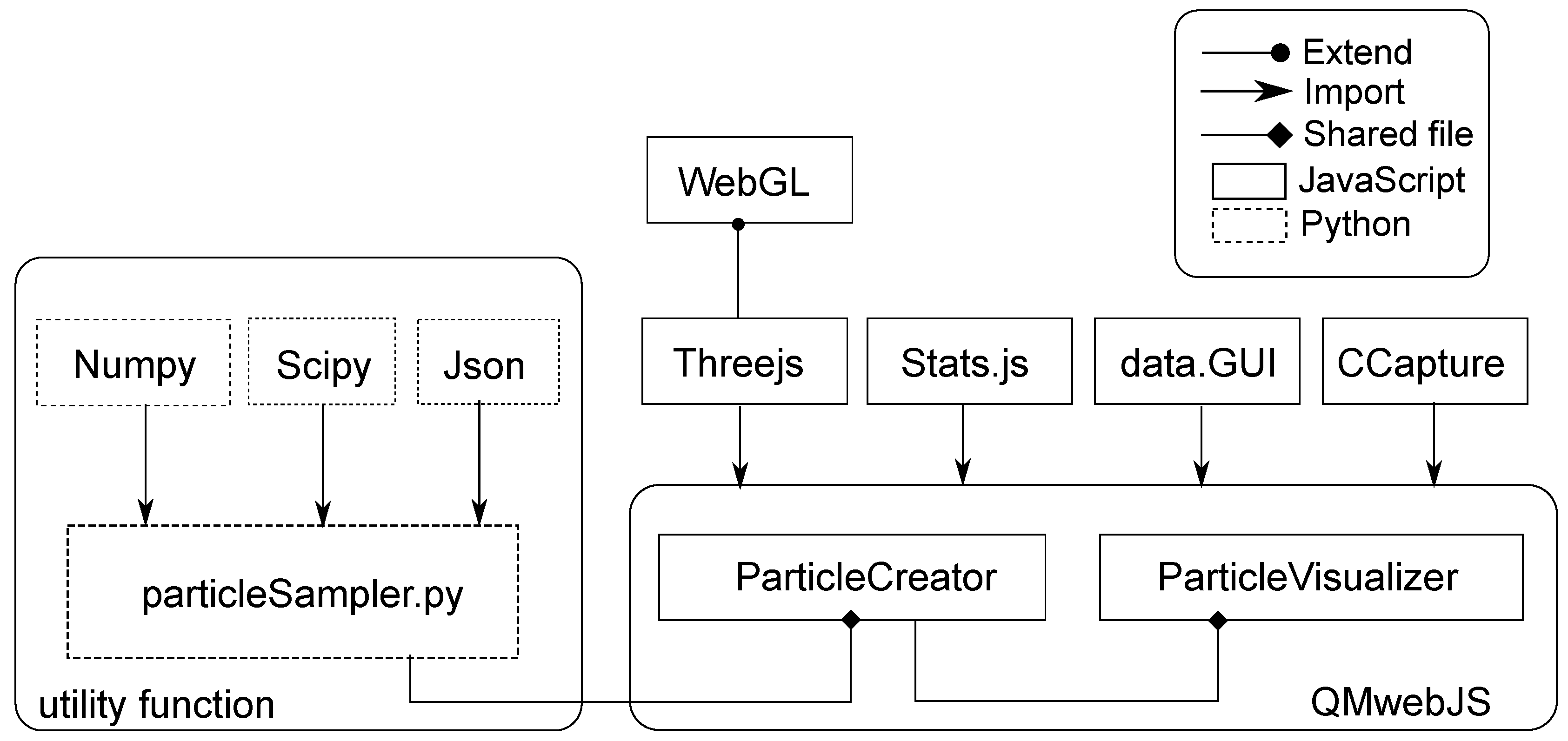
The class architecture of QMwebJS is shown in Figure 2. QMwebJS depends on the Three.js javascript library (https://threejs.org), which in turn builds upon WebGL (https://www.khronos.org/webgl/)—a standard low-level graphics library built into all modern web browsers. The Three.js library provides asynchronous event-driven functions for building menu and graphical control widgets (e.g., buttons, sliders, mouse-event handling, etc.) that bind to the low-level WebGL actions. Thus, QMwebJS consists of a customized Graphical User Interface (GUI) for creating, editing, and manipulating wavefunctions from the particle-sampling method with graphics primitives.

Apart from the dependency on Threejs and WebGL, QMwebJS uses two other javascript libraries for functionality. textitdat.GUI (github.com/dataarts/dat.gui) is a pure Javascript library that provides functionality for building graphical user interfaces (GUI) with a full range of events and callback utilities. Ccapture.js (https://github.com/spite/ccapture.js/): a pure Javascript library for capturing animations at the web without losing quality.

As seen in Figure 2, QMwebJS contains two core modules written in JavaScript that control the WebGL viewport. The first module, ParticleCreator, loads the simulation data to an internal 3D model data structure. The other module, ParticleVisualizator, relies upon WebGL and ThreeJS to display the model in a viewport, manipulate/edit the aspects of the visualization with custom callback functions.

Codeflow through QMwebJS library is shown in Figure 3, where only the most important functions are shown.

Asynchronous interaction is accomplished by the main infinite loop, (the Render Loop), which common to all similar event-driven applications. All interactive WebGL applications are designed similarly, where not only are mouse/keyboard events monitored, but also each iteration represents an independent display frame.  

1 var RenderLoop = function( )
2 {
3     requestAnimationFrame( RenderLoop );
4     stats.update();/*FPS and MS/Frame counter */
5     update( );     /*Updates if are changes   */
6     render( );     /*Renders the visualization*/
7 }
		

Listing 1: JavaScript loop code that allows the visualization to be continuously rendered, keeping the visualization alive and interactive.

Data load

1 let arrayData = [];
2 /*Function that load the 3Ddata file*/
3 let dataLoad = function( ){
4     /*Load from a folder called data3d*/
5     fetch( ’./data3d/’.concat(dataName))
6     .then(function(resp) {
7         return resp.json( );
8     })
9     .then(function(dataFile) {
10         console.log(dataFile);
11        /*Copy the 3d data into the new array*/
12        arrayData = dataFile;
13        /*Call the main function for start render*/
14        createParticles( );
15     });
16 }

Listing 2: Javascript code for .json data upload.

Placing Particles in the Viewport

The two principal functions for generating and placing the data in the 3D canvas are PlaceParticles and PlaceParticlesLowRender. Both functions share an identical main structure, shown in the Algorithm 2. As indicated, the first step is to read the particle locations and then depending upon the number of particles indicated in the QMwebJS GUI panel, these are displayed in the viewport by instantiating basic 3D objects.

Algorithm 2: Place particles.

Require: Matrix loaded with simulation data $arrayData$

Set number of particles via GUI $nParticles=N_i$

Ensure: Display simulation particles at the 3D canvas. 1: $pCount=0$ 2: while$pCount<nParticles$do 3:    $tStep\leftarrow GUI.timeStep$ 4:    $x,y,z,psi\leftarrow arrayData\left[tStep\right]\left[pCount\right](x,y,z,\mathsf{\Psi })$ 5:    $color\leftarrow calculateColor\left(psi\right)$ 6:    $pCount\leftarrow pCount+1$ 7:    ${}^1$Generate high quality particles (Listing 3). ∥${}^2$Store data in arrays (Listing 4). 8: end while 9: ${}^2$Generate high performance particles with stored data (Listing 4). 10: $CLS$ 11: $DisplayVisualization\left(\right)$

${}^{1}placeParticles\left(\right)$, ${}^{2}placeParticlesLowRender\left(\right)$

Despite their similarities, these two functions employ different methods for creating the 3D model, while possessing the same internal structure. A more detailed explanation of each is described below.

Place particles:

The placeParticles function creates icosahedrons in the 3D environment. First, a group of 3D objects is created that are an intrinsic Three.js data type for storing object arrays as groups. Next, within the main loop, the data array set to the spatial grid positions $\mathbf{r}=(x,y,z)$. As mentioned previously, particles are assigned a false color based on the value of ${|\mathsf{\Psi }|}^2$ (from the nearest grid point) in order to represent density for more effective visualizations; low density is towards blue, while high density is towards red and/or white. With this color value and point position $\mathbf{r}$, the object is added to a global array list and instantiated in the 3D viewport (see Listing 3 and accompanying detailed description).

Each particle can be represented as primitive 3D objects, so that both perspective and light effects are of very high quality. To accomplish this, the material properties are modified in order to choose a wireframe or solid object; this is done with particlesWireframed, available in the QMwebJS GUI panel. For solid objects, a primitive icosahedron is prefered over a primitive sphere; the IcosahedronBufferGeometry is a Three.js geometry with less impact on performance due to fewer faces compared to a sphere. To further improve graphics performance, the number of icosahedron faces can be set. Once the loop is finished, the previous visualization with clear_scene is eliminated and the set of objects created in this time step is added to the 3D canvas.

1 /*Create a new material with Psi color data*/
2 var material =  new THREE.MeshLambertMaterial( {
3 color: calculate_color_by_amplitude_hex(psi,psiMin,psiMax),
4  wireframe: particlesWireframed} );
5 /*Create a new Icosahedron object*/
6 var geometry = new THREE.IcosahedronBufferGeometry(objectSize, 0 )
7 /*Generate a particle object*/
8 var particle = new THREE.Mesh( geometry, material );
9 /*Set the 3D data position*/
10 particle.position.set( x, y, z );
        

Listing 3: Javascript code for generating and placing the particles at the 3D canvas using Icosahedron geometries.

Place Particles Low Render

The placeParticlesLowRender function creates particles with the best render performance, since these are actually 2D objects, but  with software methods that correctly treat perspective depending upon camera angles. To create these objects, the following steps in the function are taken. First, the function creates a geometry buffer. All the particles will be assigned to this buffer after they have been created. Next, two vectors are created to store the 3D positions and the colors. The main loop for reading data from the matrix is identical to the code in the previous section. However, in this function the position and color data (rgb- format) are stored into the arrays. This algorithm of memory buffering loads the data into the viewport, as shown in Listing 4. The last function of Listing 4 assigns the position and color from within the loop. Then, a material is created that, together with the geometry buffer, will be used to create the particles. The 2D particles are created using an original data type of Threejs, called Points.

1 /*Add to geometry positions and colors*/
2 geometry.addAttribute( ’position’, new THREE.Float32BufferAttribute( positions, 3 ) );
3 geometry.addAttribute( ’color’, new THREE.Float32BufferAttribute( colors, 3, true) );
4 /*Create a material*/
5 var material = new THREE.PointsMaterial( {
6         size: particleSize, vertexColors: THREE.VertexColors } );
7 /*Generate a group of points with geometry and material*/
8 points = new THREE.Points( geometry, material );
      

Listing 4: Javascript code for generating and placing the particles at the 3D canvas using Points buffer.

In the previous Listing 3, 3D data objects were created with IcosahedronBufferGeometry. Along the timeline, once the model formed by points (see Listing 4) is created, the previous visualization is eliminated and the points are added to the 3D canvas.

4. The QMwebJS Visualization Environment

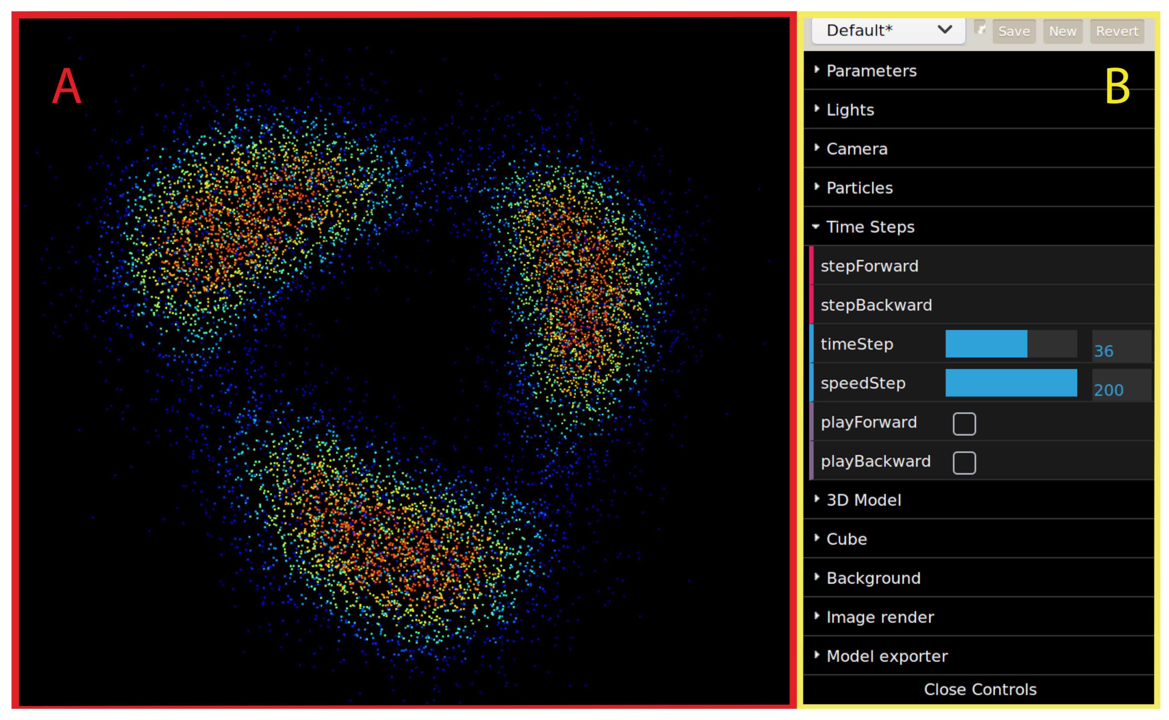
Figure 4 shows the QMwebJS environment. This environment is divided into two parts: the display viewport canvas area (A) and the GUI panel (B). Objects in the viewport can be manipulated in an expected and intuitive manner for 3D viewers by zoom, rotation, and translation. The panel is divided into several expandable tabs for interacting and modifying the model. Other utilities such as loading and exporting models are also available through the GUI panel.

Several “tabs” are available on the lateral side panel to adjust viewport parameters. Figure 4 shows these GUI controls. A brief description follows, while a more complete description can be found in the Supplementary Materials.

Two important parameters in any 3D editor are the position and value of the lighting, and the viewing angle of the camera. These parameters are controlled from the Light and Camera tab. In this way, full control over the light position, direction, and value is adjustable. The viewing camera position is also available from this tab.

The Particles tab (Figure 4) controls the number of particles, the particle size, and also color scaling. In the Time Steps tab, a scrubber bar as well as text input provides fine control over visualization of frames along the timeline. All changes to the model are reflected in real time in the display view with low latency, which is achieved by using a memory efficient data type, called the Point Buffer Geometry. In this way, users can interactively customize visualization parameters (colors, point sizes, etc.) using the other options to adapt the 3D model to their objectives.

The 3D Model tab allows users to change the quality of the 3D model, selecting details of the icosahedron meshes for the basic particle geometry. Thus, to improve performance, faces of polygons can be eliminated or wireframe icosahedrons can be used. For example, disabling the occluded polygon faces can significantly improve memory performance which otherwise would require more processing.

In Cube and Background tabs of Figure 4 allow users to change background color as well as to toggle a wireframe cube useful for perceiving 3D orientation. The Image render tab configures and generates the renders to download images from the simulation. Here also, the 3D models can be exported to be viewed in any standard 3D software editor/viewer.

4.1. Rendering Performance of 3D Objects

This section describes the practical rationale of choosing between two types of 3D objects with respect to overall capability and performance issues. The two main objects used to represent particles are the Points Buffer (PB) and the Mesh Icosahedron (MI-MIW). Tests were performed to determine how much memory and processing is needed for each depending upon the total number of particles to be rendered.

Figure 5 shows comparisons between these two data type methods utilized for each of the particles: the point buffer (PB) geometry and the mesh icosahedron (MI-MIW) geometries. The points buffer geometry method (Figure 5A) is a memory-optimized geometric object that are stored as 2D flat objects; the associated methods guarantee that these objects always are shown as front-facing with respect to the camera position. While memory efficient (e.g., ${10}^6$ points do not cause the slightest latency load on graphic performance), these objects do not reflect light as a 3D sphere would; this is especially noticeable at close distance where points are seen as small flat squares (see the zoom 6x of Figure 5A). For many situations with many particles, this produces quite adequate visual representations.

For full 3D depth, the Mesh Icosahedron Figure 5B and the Mesh Icosahedron wire-framed Figure 5C are of interest. The fact that these objects are three-dimensional meshes means that textures and reflective properties can be applied to them. Also, the number of faces of the polyhedron can be adjusted, starting from the minimum defined by WebGL (a 20 faced Icosahedron) in order to emulate the volume of spheres, yet retain graphic and memory performance.

Figure 6, shows that with the PB it is necessary to double or even triple the number of objects used to achieve a quality visualization similar to those of the MI or the MIW. As described, this is because the PB consists of a set of 2D points distributed across the three-dimensional grid that have minimal impact on memory. However, in the case of the MIs, the 3D quality is better but the impact on memory and rendering is larger. Comparing the MI and MIW some differences can also be seen. The MIW has smoother visualization when the model is seen from a certain distance. That is because the occluded objects could be seen through the wireframed structure of the icosahedrons when wireframe mode in enabled. When the camera is closer, the MI has best results as shown at Figure 5.

In practice, in order to optimize graphic latency, it is often useful to use the PB during editing tasks, where speed is required for parameter adjustment, while for producing production level models, the full 3D polygon and wireframe objects are used.

4.2. Performance

Figure 7 shows a comparison of the memory and render response times as a function of the number of particles used for the different object types. The impact on memory (Figure 7A) of the PB (Points Buffer) is much smaller compared to that used by the MI (Mesh Icosahedron Geometry) or the MIW (Mesh Icosahedron Geometry Wireframed). In the previous section (Figure 6), it was shown that the number of the PB with respect to that of MI should be doubled or tripled in order to achieve similar performance.

The results in terms of the rendering time demonstrate the difficulty of working with the MI or MIW above a certain number of particles. While difficult to quantify, the sense of response latency is noticed considerably in animations when the fps is below 24. From Figure 7B that compares frame rates for the PB and MI, regimes for each can be established for retaining reasonable response. In particular, the PB is the best option when low memory utilization and maximum fluidity are intended. When using this low render method, it is possible to attain 60 frames per second during the editing, thereby producing smooth and fluid movement. On the other hand, the MI and MIW should be used for tasks that require the highest display quality, that for modest hardware would suffer from lower frame rates during editing.

Another factor to consider is the size of the 3D exported models. A comparison with between the OBJ and the GLTF is shown in Figure 8. While the OBJ model format is a more widely used standard, this comparison shows that GLTF provides better memory performance.

5. Use in a Quantum Mechanics Course

We can envisage two main strategies that could profit from the use of QMwebJS in an undergraduate educational context. For this discussion, we provide three illustrative examples from relevant quantum systems. While assessing the student’s overall learning efficiency with this software would have great value, such a cohort study is beyond the scope of the present work. Nonetheless, several studies are available that establish some foundations for how such a case study could be carried out (see References [7,24,25] for cases that make use of questionnaires to investigate the impact of different methodologies in the context of quantum physics education).

The first strategy is that of creating animations that can be used for demonstrations in the classroom or to produce models to be stored in a repository accessible to students. As described, these models could be accessed by the students and viewed interactively within QMwebJS or any other 3D viewer to explore different cases of interest.

In Reference [26], the authors describe the value of animations to help students build mental representations of concepts related to quantum mechanics. In this spirit, the teacher would produce and choose illustrative examples of wavefunction dynamics, that may be difficult to conceive using more standard techniques. These interactive visualizations would complement written notes or books, making these concepts come to life, by  providing clear display of the probabilistic time evolution of 3D distributions.

The second strategy, for which the QMwebJS library would be especially convenient, is that of inquiry-based learning. The value of research-based methods for the students’ understanding of particular quantum concepts was highlighted in Reference [27]. The accessibility, adaptability, and simplicity of the visualization tool can allow students to pursue their own projects and create their own models without investing much effort in getting started with the software details. The possibility of sharing the models would be useful to distribute their results to their teachers or colleagues. Notice, by the way, that apart from the aforementioned plotting of ${|\mathsf{\Psi }(t,\mathbf{x})|}^2$, one can also depict the probability distribution in Fourier space $|\tilde{\mathsf{\Psi }}{(t,\mathbf{p})|}^2$. Comparing the direct space and momentum space models for the same wavefunction, a qualitative visual understanding of the uncertainty principle could be developed.

Both strategies would greatly benefit by combining QMwebJS with a simulation module to integrate the time-dependent 3D Schrödinger equation for a given potential and initial condition, in order to produce the input data to be visualized. In fact, we presented a Python-based tool of this sort in Reference [28] for the 1D and 2D cases, but it can be readily generalized to the 3D case (in fact, 3D was not included in Reference [28] mainly because of the difficulties in automatically producing attractive and informative 3D plots). In the Supplementary Materials (also see http://www.parvis3d.org.es/), we provide the code and simulation results of the examples shown below, that are 3D adaptation of the examples given in Reference [28].

Let us now present three examples that can serve to illustrate quantum concepts that are typically taught in undergraduate courses: the decay of an excited eigenfunction, quantum tunneling and interference of the wavefunction. In the following, we consider the time Schrödinger equation written in adimensional form:

$$i\frac{\partial \mathsf{\Psi }(t,\mathbf{x})}{\partial t}=-\frac{1}{2}{\nabla }^2\mathsf{\Psi }(t,\mathbf{x})+V\left(\mathbf{x}\right)\mathsf{\Psi }(t,\mathbf{x}).$$

(1)

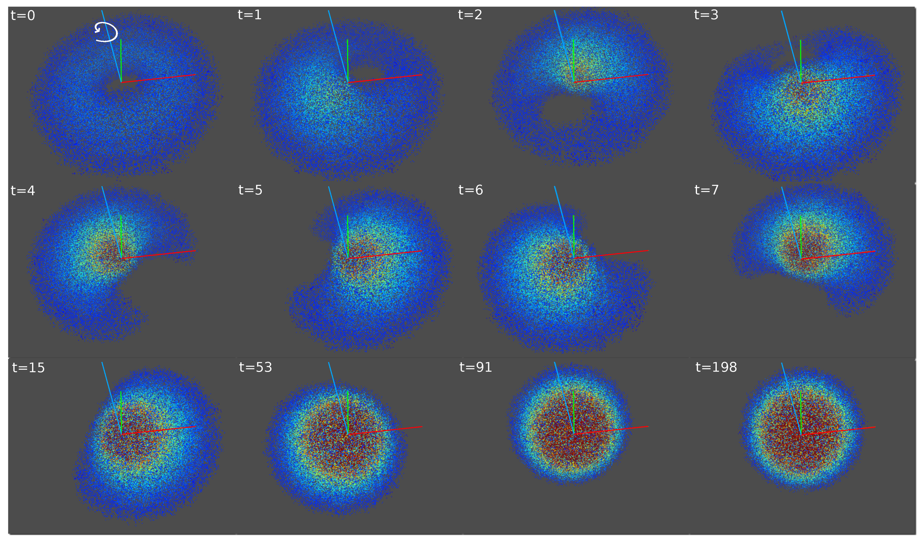
For the first example, let us consider how an excited hydrogen atom decays to a lower energy state, a process usually studied in connection with quantum perturbation theory. Taking $V=-1/r$, the eigenstates, discussed in innumerable texts on quantum mechanics, depend on three quantum numbers $n,l,m$ and form an orthonormal basis that can be written as:

$${\mathsf{\Psi }}_{nlm}=e^{-i{E}_{n}t}{R}_{nl}\left(r\right)Y_{lm}(\theta ,\phi ),$$

(2)

where $r,\theta ,\phi$ are spherical coordinates, $E_n=-\frac{1}{2n^2}$ are the quantized energies, $Y_{lm}(\theta ,\phi )$ are spherical harmonics and the radial part of the wavefunction $R_{nl}\left(r\right)$ is the product of an exponential $e^{-r/n}$ and an associated Laguerre polynomial. Consider the following expression for the temporal evolution of the wavefunction decaying from an initial state parameterized by $n_i,l_i,m_i$ to a final state with $n_f,l_f,m_f$

$$\mathsf{\Psi }(t,\mathbf{x})=e^{-\frac{t}{2\tau }}{\mathsf{\Psi }}_{n_i{l}_i{m}_i}+\sqrt{1-e^{-\frac{t}{\tau }}}{\mathsf{\Psi }}_{n_f{l}_f{m}_f},$$

(3)

where $\tau$ is the decay time of the transition. Notice that directly including the time exponential in the wavefunction is not exact in general but it is a good approximation to the correct behavior. Discussing this subtle issue is not our goal here but we refer the interested reader to References [29,30]. Considering the actual dimensionful parameters, the decay time of the hydrogen atom excited states for transitions mediated by the electric dipole moment is in the order of the nanosecond, whereas the inverse of the frequency appearing in the complex exponential $ħ/E_n$ is of the order of tens or hundreds of attoseconds for the lowest-lying states. Thus, the adimensional $\tau$ is a huge number around ${10}^8$. For visualization convenience, a smaller value of the order of ${10}^3$ was used to build this simple model.

Some images from the simulation are depicted in Figure 9. Notice that watching this animation can help to reconcile the quantum concept of quantized excited states decay and the excess energy is released as a photon with the classical concept accelerated charges emit electromagnetic radiation. Indeed, it can be appreciated that the probability distribution of the electric charge shifts in time in a such a way that it could be semi-classically identified with a microscopic circular antenna with a typical oscillation frequency of $(E_{n_i}-E_{n_f})$.

For the second example, let us consider a potential with two adjacent truncated harmonic potentials centered at positions ${\mathbf{x}}_1$, ${\mathbf{x}}_2$:

$$V=\frac{1}{2}min(|\mathbf{x}-{\mathbf{x}}_1{|}^2,|\mathbf{x}-{\mathbf{x}}_2{|}^2)$$

(4)

and take as initial condition the would-be ground state of one of the harmonic wells, if it were isolated from the other one:

$$\mathsf{\Psi }(t=0,\mathbf{x})={\pi }^{-\frac{3}{4}}exp\left(-\frac{1}{2}{|\mathbf{x}-{\mathbf{x}}_1|}^2\right).$$

(5)

In typical quantum mechanics courses, students learn that this is not an eigenstate of the full system and, that, therefore, the probability distribution will evolve. In particular, it will tunnel from one of the potential minima to the other, with a tunneling rate depending on the height of the barrier between them (in this case, depending on $|{\mathbf{x}}_1-{\mathbf{x}}_2|$).

Some images of the visualization of this process generated with QMwebJS are displayed in Figure 10. The particle representation shows how there is a probability current from one minimum to the other, providing a qualitative illustration of the continuity equation of quantum mechanics (this particular feature is much harder to visualize with iso-surface plots). Notice that the particles in any plot can be heuristically regarded as follows—making a measurement of position would give the position of one of the particles chosen at random amongst the whole set (this corresponds to the actual prediction of the quantum theory in the limit of infinite number of particles). Thus, the particle sampling method is particularly adequate to depict probability fluxes.

The third example depicts quantum interference, shown in Figure 11. The wavefunction is initially divided into four separate gaussian wavepackets. They start expanding due to the diffraction term and they eventually come into contact producing a characteristic interference pattern. The setup is a sort of quantum multiple-slit numerical experiment. Again, the particle representation is useful here for the physical understanding. Take the image after some time when the fringe pattern has been formed. The distribution of N particles resembles the result of repeating the multiple-slit experiment for a single electron N times and measuring the electron position always at that particular time.

6. Conclusions and Outlook

Here, we presented a software tool to facilitate the interactive representation and the sharing of the time evolution of three dimensional probability distributions. The visualization algorithm employs a particle sampling method and can be used on a cloud microservice accessible from any standard web browser, or run locally by just opening an html file in a web browser. The library is written in JavaScript, with some helper utilities in Python and relies on a number of standard libraries and freeware applications. We provide the open source library and a few 3D models to server as illustrative examples.

Throughout, we have argued that, mostly thanks to its accessibility, usage simplicity and adaptability, QMwebJS can be a useful resource to teach quantum mechanics courses, both for graphical demonstrations prepared by the teacher or as a useful application for student projects. In combination with a simulation module to integrate the 3D time-dependent Schrödinger equation (e.g., by adapting our previous contribution [28] to the 3D case), it may open many possibilities for inquiry-based learning of particular aspects of quantum mechanics. Certainly, it would be interesting to directly test, using physics education research methods, the influence of the utilisation of the software in improving the student understanding and motivation. If the present proposal turns out to be successful, it could be interesting to generalize the software to depict similar methods with vector fields (e.g., the linear momentum density distribution), combinations of spatial wavefunctions and internal degrees of freedom (e.g., spin) or other quantities of interest.

Finally, it is worth commenting that the application presented here might be profitable beyond educational contexts. We envisage its possible adequacy for the diffusion of research results, in particular in relation to the simulation of the dynamics of 3D nonlinear waves.

References

- De Jong, T.; Linn, M.C.; Zacharia, Z.C. Physical and virtual laboratories in science and engineering education. Science 2013, 340, 305–308. [Google Scholar] [CrossRef] [Green Version]
- Rau, M.A. Conditions for the Effectiveness of Multiple Visual Representations in Enhancing STEM Learning. Educ. Psychol. Rev. 2017, 29, 717–761. [Google Scholar] [CrossRef]
- Ainsworth, S. The Educational Value of Multiple-representations when Learning Complex Scientific Concepts. In Visualization: Theory and Practice in Science Education. Models and Modeling in Science Education; Gilbert, J.K., Reiner, M., Nakhleh, M., Eds.; Springer: Dordrecht, The Netherlands, 2008; Volume 3. [Google Scholar] [CrossRef]
- Hatherly, P.A.; Jordan, S.E.; Cayless, A. Interactive screen experiments-innovative virtual laboratories for distance learners. Eur. J. Phys. 2009, 30, 751–762. [Google Scholar] [CrossRef]
- Galan, D.; Heradio, R.; de la Torre, L.; Dormido, S.; Esquembre, F. The experiment editor: Supporting inquiry-based learning with virtual labs. Eur. J. Phys. 2017, 38, 035702. [Google Scholar] [CrossRef]
- Zacharia, Z.C.; Olympiou, G.; Papaevripidou, M. Effects of experimenting with physical and virtual manipulatives on students’ conceptual understanding in heat and temperature. J. Res. Sci. Teach. 2008, 45, 1021–1035. [Google Scholar] [CrossRef]
- Chhabra, M.; Das, R. Quantum mechanical wavefunction: Visualization at undergraduate level. Eur. J. Phys. 2016, 38, 015404. [Google Scholar] [CrossRef]
- Orquin, I.; Garcia-March, M.A.; de Cordoba, P.F.; Urcheguía, J.F.; Monsoriu, J.A. Introductory quantum physics courses using a LabVIEW multimedia module. Comput. Appl. Eng. Educ. 2007, 15, 124–133. [Google Scholar] [CrossRef] [Green Version]
- Passante, G.; Kohnle, A. Enhancing student visual understanding of the time evolution of quantum systems. Phys. Rev. Phys. Educ. Res. 2019, 15, 010110. [Google Scholar] [CrossRef] [Green Version]
- Johnson, J.L. Visualization of wavefunctions of the ionized hydrogen molecule. J. Chem. Educ. 2004, 81, 1535. [Google Scholar] [CrossRef] [Green Version]
- Figueiras, E.; Olivieri, D.; Paredes, A.; Michinel, H. QMBlender: Particle-based visualization of 3D quantum wave function dynamics. J. Comput. Sci. 2019, 35, 44–56. [Google Scholar] [CrossRef]
- Hansen, C.D.; Johnson, C.R. (Eds.) The Visualization Handbook; Elsevier Butterworth-Heinemann: Oxford, UK, 2005. [Google Scholar]
- Lipsa, D.R.; Laramee, R.S.; Cox, S.J.; Roberts, J.C.; Walker, R.; Borkin, M.A.; Pfister, H. Visualization for the physical sciences. In Computer Graphics Forum; Blackwell Publishing Ltd.: Oxford, UK, 2012; Volume 31, pp. 2317–2347. [Google Scholar]
- Telea, A.C. Data Visualization: Principles and Practice; AK Peters: Natick, MA, USA; CRC Press: Boca Raton, FL, USA, 2014. [Google Scholar]
- Kruger, J.; Kipfer, P.; Konclratieva, P.; Westermann, R. A particle system for interactive visualization of 3D flows. IEEE Trans. Vis. Comput. Graph. 2005, 11, 744–756. [Google Scholar] [CrossRef] [PubMed]
- Raji, M.; Hota, A.; Hobson, T.; Huang, J. Scientific Visualization as a Microservice. IEEE Trans. Vis. Comput. Graph. 2018. [Google Scholar] [CrossRef]
- Diblen, F.; Attema, J.; Bakhshi, R.; Caron, S.; Hendriks, L.; Stienen, B. spot: Open Source framework for scientific data repository and interactive visualization. SoftwareX 2019, 9, 328–331. [Google Scholar] [CrossRef]
- Liu, L.; Silver, D.; Bemis, K. Visualizing Three-Dimensional Ocean Eddies in Web Browsers. IEEE Access 2019, 7, 44734–44747. [Google Scholar] [CrossRef]
- Liu, D.; Peng, J.; Wang, Y.; Huang, M.; He, Q.; Yan, Y.; Ma, B.; Yue, C.; Xie, Y. Implementation of interactive three-dimensional visualization of air pollutants using WebGL. Environ. Model. Softw. 2019, 114, 188–194. [Google Scholar] [CrossRef]
- Evangelidis, K.; Papadopoulos, T.; Papatheodorou, K.; Mastorokostas, P.; Hilas, C. 3D Geospatial Visualizations. Comput. Geosci. 2018, 111, 200–212. [Google Scholar] [CrossRef]
- Carrillo-Tripp, M.; Alvarez-Rivera, L.; Lara-Ramírez, O.I.; Becerra-Toledo, F.J.; Vega-Ramírez, A.; Quijas-Valades, E.; González-Zavala, E.; González-Vázquez, J.C.; García-Vieyra, J.; Santoyo-Rivera, N.B.; et al. HTMoL: Full-stack solution for remote access, visualization, and analysis of molecular dynamics trajectory data. J. Comput.-Aided Mol. Des. 2018, 32, 869–876. [Google Scholar] [CrossRef] [Green Version]
- Bracci, M.; Tarini, M.; Pietroni, N.; Livesu, M.; Cignoni, P. HexaLab.net: An online viewer for hexahedral meshes. Comput.-Aided Des. 2019, 110, 24–36. [Google Scholar] [CrossRef] [Green Version]
- Kaboudian, A.; Cherry, E.M.; Fenton, F.H. Large-scale interactive numerical experiments of chaos, solitons and fractals in real time via GPU in a web browser. Chaos Solitons Fractals 2019, 121, 6–29. [Google Scholar] [CrossRef]
- Marshman, E.; Singh, C. Investigating and improving student understanding of the probability distributions for measuring physical observables in quantum mechanics. Eur. J. Phys. 2017, 38, 025705. [Google Scholar] [CrossRef] [Green Version]
- Marshman, E.; Singh, C. Investigating and improving student understanding of the expectation values of observables in quantum mechanics. Eur. J. Phys. 2017, 38, 045701. [Google Scholar] [CrossRef] [Green Version]
- Kohnle, A.; Douglass, M.; Edwards, T.J.; Gillies, A.D.; Hooley, C.A.; Sinclair, B.D. Developing and evaluating animations for teaching quantum mechanics concepts. Eur. J. Phys. 2010, 31, 1441. [Google Scholar] [CrossRef]
- Zhu, G.; Singh, C. Improving students’ understanding of quantum measurement. II. Development of research-based learning tools. Phys. Rev. Spec.-Top.-Phys. Educ. Res. 2012, 8, 010118. [Google Scholar] [CrossRef] [Green Version]
- Figueiras, E.; Olivieri, D.; Paredes, A.; Michinel, H. An open source virtual laboratory for the Schrödinger equation. Eur. J. Phys. 2018, 39, 055802. [Google Scholar] [CrossRef]
- Peshkin, M.; Volya, A.; Zelevinsky, V. Non-exponential and oscillatory decays in quantum mechanics. EPL (Europhys. Lett.) 2014, 107, 40001. [Google Scholar] [CrossRef] [Green Version]
- Merzbacher, E. Quantum Mechanics; John Wiley & Sons. Inc.: New York, NY, USA, 1998. [Google Scholar]
Figure 1.
Steps of the data workflow for using QMwebJS.
Figure 2.
The QMwebJS system architecture and libraries.
Figure 3.
Diagram that shows the code workflow from the data load to the 3D model creation.
Figure 4.
Example of the Graphical User Interface (GUI). The visualization canvas of QMwebJS is shown in (A); the side-panel of the GUI with the tab Time Steps expanded shown in (B).
Figure 5.
Object representation comparisons for the same wavefunction example. The subfigures illustrate: (A) the point buffer primitives, (B) the mesh icosahedron geometry primitives, and (C) the wireframe mesh icosahedron primitives. Each representation is shown with 3× and 6× zoom for clarity (bottom row).
Figure 6.
Comparison between the Point Buffer Geometry (PB), the Mesh Icosahedron Geometry (MI) and the Mesh Icosahedron Geometry Wireframed (MIW) representing the same data with different number of particles.
Figure 7.
(A) Comparison of the memory usage using the Points Buffer and the two Mesh Icosahedrons Geometry objects. (B) Comparison of time used to render a frame and frames per second using the Points Buffer and the two Mesh Icosahedron Geometry objects.
Figure 8.
Size comparison of 3D model file using GLTF and OBJ formats.
Figure 9.
Illustration of the evolution of the wavefunction during a dipolar decay of an excited eigenstate of the hydrogen atom.
Figure 10.
Illustration of the evolution of the wavefunction during a quantum tunneling process.
Figure 11.
Illustration of the evolution of a wavefunction leading to quantum interference.
© 2020 by the authors. Licensee MDPI, Basel, Switzerland. This article is an open access article distributed under the terms and conditions of the Creative Commons Attribution (CC BY) license (http://creativecommons.org/licenses/by/4.0/).
Share and Cite
MDPI and ACS Style
Figueiras, E.; N. Olivieri, D.; Paredes, A.; Michinel, H. QMwebJS—An Open Source Software Tool to Visualize and Share Time-Evolving Three-Dimensional Wavefunctions. Mathematics 2020, 8, 430. https://doi.org/10.3390/math8030430
AMA Style
Figueiras E, N. Olivieri D, Paredes A, Michinel H. QMwebJS—An Open Source Software Tool to Visualize and Share Time-Evolving Three-Dimensional Wavefunctions. Mathematics. 2020; 8(3):430. https://doi.org/10.3390/math8030430
Chicago/Turabian StyleFigueiras, Edgar, David N. Olivieri, Angel Paredes, and Humberto Michinel. 2020. "QMwebJS—An Open Source Software Tool to Visualize and Share Time-Evolving Three-Dimensional Wavefunctions" Mathematics 8, no. 3: 430. https://doi.org/10.3390/math8030430
Note that from the first issue of 2016, this journal uses article numbers instead of page numbers. See further details here.