A db-Scan Hybrid Algorithm: An Application to the Multidimensional Knapsack Problem

Abstract

This article proposes a hybrid algorithm that makes use of the db-scan unsupervised learning technique to obtain binary versions of continuous swarm intelligence algorithms. These binary versions are then applied to large instances of the well-known multidimensional knapsack problem. The contribution of the db-scan operator to the binarization process is systematically studied. For this, two random operators are built that serve as a baseline for comparison. Once the contribution is established, the db-scan operator is compared with two other binarization methods that have satisfactorily solved the multidimensional knapsack problem. The first method uses the unsupervised learning technique k-means as a binarization method. The second makes use of transfer functions as a mechanism to generate binary versions. The results show that the hybrid algorithm using db-scan produces more consistent results compared to transfer function (TF) and random operators.

1. Introduction

With the incorporation of technologies such as big data and the Internet of Things, the concept of real-time decisions has become relevant at the industrial level. Each of these decisions can be modeled as an optimization problem or, in many cases, a combinatorial optimization problem (COP). Examples of COPs are found in different areas: machine learning [1], transportation [2], facility layout design [3], logistics [4], scheduling problems [2,5], resource allocation [6,7], routing problems [8], robotics applications [9], image analysis [10], engineering design problems [11], fault diagnosis of machinery [12], and manufacturing problems [13], among others. If the problem is large, metaheuristics have been a good approximation to obtain adequate solutions. However, having a greater amount of data and requiring solutions in close to real time for some cases motivates us to continue strengthening the methods that address these problems.

One way to classify metaheuristics is according to the search space in which they work. In that sense, we have metaheuristics that work in continuous spaces, discrete spaces, and mixed spaces [14]. An important line of inspiration for metaheuristic algorithms is natural phenomena, many of which develop in a continuous space. Examples of metaheuristics inspired by natural phenomena in continuous spaces include particle swarm optimization [15], black hole optimization [16], cuckoo search [17], the bat algorithm [18], the firefly algorithm [19], the fruitfly algorithm [20], the artificial fish swarm [21], and the gravitational search algorithm [22]. The design of binary versions of these algorithms entails important challenges when preserving their intensification and diversification properties [14]. The details of binarization methods are specified in Section 3.

A strategy that has strengthened the results of metaheuristic algorithms has been the hybridization of these with techniques that come from the same or other areas. The main hybridization proposals found in the literature are the following: (i) matheuristics, which combine heuristics or metaheuristics with mathematical programming [23]; (ii) hybrid heuristics, a combination between different heuristic or metaheuristic methods [24]; (iii) simheuristics, where simulation and metaheuristics are combined together to solve a problem [25]; and (iv) Integration between metaheuristic algorithms and machine learning techniques. The last, hybridization between the areas of machine learning and metaheuristic algorithms, is an emerging research line in the areas of computer science and operational research. We find that hybridization occurs mainly with two intentions. The first is with the goal that metaheuristics will help machine learning algorithms improve their results (for example, [26,27]). The second intention is that machine learning techniques will be used to strengthen metaheuristic algorithms (for example, [28,29]). The details of the hybridization forms are specified in Section 4.

This article is inspired by the research lines mentioned above. A hybrid algorithm is designed that explores the application of a machine learning algorithm in a binarization operator to allow continuous metaheuristics to address combinatorial optimization problems. The contributions of this work are detailed below:

• A machine learning technique is used with the objective of obtaining binary versions of metaheuristics defined and used in continuous optimization to tackle COPs in a simple and effective way. To perform the binarization process, this algorithm uses db-scan, which corresponds to an unsupervised learning algorithm. The selected metaheuristics are particle swarm optimization (PSO) and cuckoo search (CS). Their selection is based on the fact that they have been frequently used in solving continuous optimization problems and their parameterization is relatively simple, which allows us to focus on the binarization process.
• The multidimensional knapsack problem (MKP) was used to check the performance of the obtained binary versions. MKP was chosen because it is a problem extensively studied in the literature therefore we have specific instances making it easy to evaluate our hybrid algorithm. The details and applications of MKP are expanded on in Section 2.
• Two random operators are designed in order to define a baseline and quantify the contribution of the hybrid algorithm that uses db-scan in the binarization process. Additionally, to make the comparison more robust, the performance of our hybrid algorithm was evaluated with methods that use k-means and transfer functions (TF) as binarization mechanisms.

This article is organized in the following sections. The definition of MKP is detailed in Section 2. Subsequently, the state-of-the-art of the main binarization and hybridization techniques between machine learning and metaheuristics are developed in Section 3. The detail of the proposed hybrid binarization algorithm is described in Section 4. In Section 5, we study the contribution of the db-scan operator to the binarization process. Additionally, in this same section, the proposed hybrid algorithm is compared with the binarization techniques that use TF and k-means. Finally, the main conclusions and future lines of investigation are detailed in Section 6.

2. Multidimensional Knapsack Problem

Due to having a large number of applications and $\mathcal{NP}$-hard computational complexity, a major research effort has been dedicated to the MKP. This optimization problem has been addressed by different types of techniques. Examples of exact algorithms that have efficiently resolved the MKP are found in [30,31]. There are also hybrid algorithms where exact algorithms are combined with depth-first search [32] or with variable fixation [33]. However, exact algorithms are capable of producing optimal solutions for small and medium-sized instances, usually with a number of variables $n\le 250$ and a number of restrictions $m\le 10$ [32,33]. This makes MKP an interesting problem for metaheuristics to address.

In the case of metaheuristics, there are several algorithms that have addressed the MKP. A modification of the harmony search algorithm that redesigns the memory rule and improves exploration capabilities was proposed in [34]. A binary artificial algae algorithm was designed in [35] that uses transfer functions to perform binarization in addition to incorporating a local search operator. A hybrid algorithm based on the k-means technique was proposed in [29]. Additionally, this algorithm incorporates local perturbation and search operators. In [36], a binary multiverse optimizer was designed to address medium-sized problems. This multiverse algorithm uses a transfer function mechanism to perform binarization. Finally, a two-phase tabu-evolutionary algorithm was developed by Lai et al. [37] to address large instances of the MKP.

Let $N=\{1,2,\dots ,n\}$ be a set of n elements and $M=\{1,2,\dots ,m\}$ be a set of m resources with capacity limit $b_i$ for each resource $i\in M$. Then, each element j has profit $p_j$ and consumes an amount of resources $c_{ij}$. The MKP consists of selecting a subset of elements such that the limit capacity of each resource is not exceeded while the profit of the selected elements is maximized. Formally, the problem is defined as follows:

$$\mathrm{Maximize}P(x_1,\dots ,x_n)=\sum _{j=1}^n{p}_j{x}_j,$$

(1)

subject to:

$$\sum _{j=1}^n{c}_{ij}{x}_j\le b_i,i\in \{1,\dots ,m\}.$$

(2)

$$x_{ij}\in \{0,1\},$$

(3)

where $b_i$ corresponds to the capacity limitation of resource $i\in M$. Each element $j\in N$ has a requirement of $c_{ij}$ regarding resource i as well as a benefit $p_j$. Moreover, $x_j\in \{0,1\}$ indicates whether the element j is in the knapsack, $j\in \{1,\dots ,n\}$, $c_{ij}\ge 0$, $p_j>0$, $b_j>0$, n corresponds to the number of items, and m is the number of knapsack constraints.

As mentioned above, the MKP has numerous applications. MKP modeling has been used in project selection and capital budgeting [38] applications as well as in the delivery of groceries in vehicles with multiple compartments [39] and the daily photographic scheduling problem of an Earth observation satellite [40]. Another interesting problem related to the MKP is the shelf space allocation problem [41]. Additionally, we found applications in the allocation of databases and processors in distributed data processing [42].

3. Related Work

3.1. Related Binarization Work

Because many processes of nature that are modeled in continuous spaces have inspired metaheuristic algorithms, there are a large number of these that are designed to work in continuous spaces. In particular, the metaheuristics cuckoo search (CS) and particle swarm optimization (PSO) have been widely used in solving continuous problems. However, there are a large number of combinatorial optimization problems, where a significant number of these are $\mathcal{NP}$-hard type. This motivates the search for robust methods that allow algorithms that operate in continuous spaces to tackle combinatorial optimization problems.

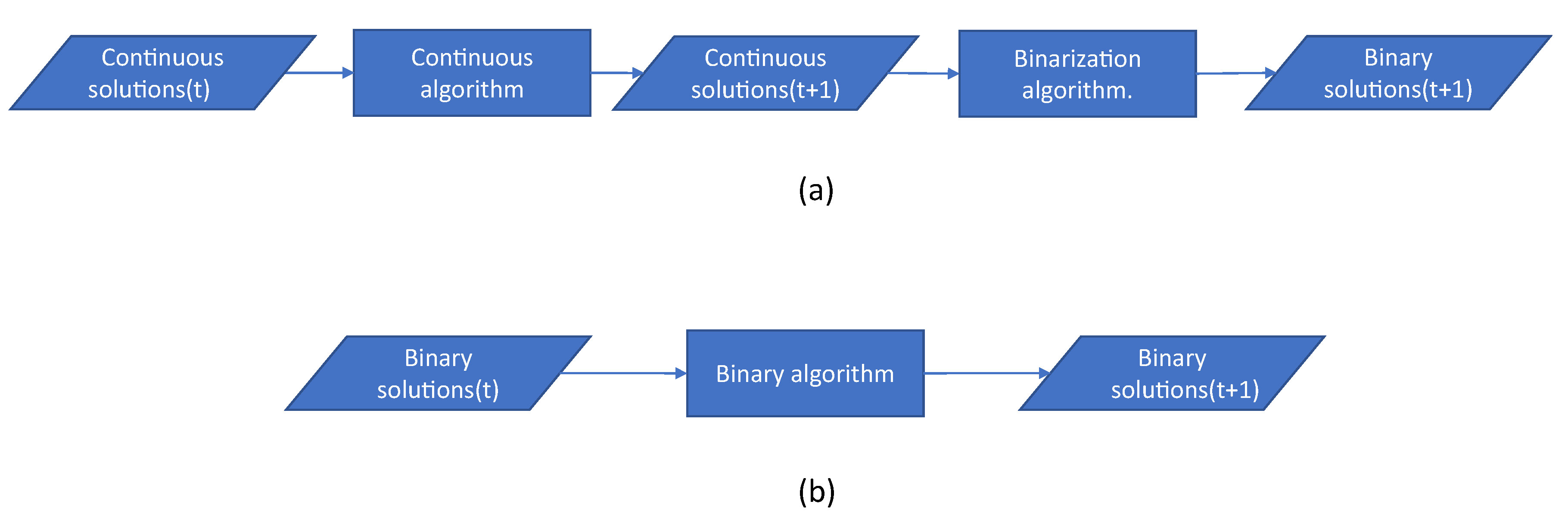
When developing a classification of existing binarization techniques, two large groups [14] are defined. The first group designs an adaptation of a continuous algorithm to work in binary environments. This adaptation usually turns out to be specific to the metaheuristic algorithm and the problem that is being solved. We call this group the specific binarizations. The second group separates the binarization process from the metaheuristic algorithm. Therefore, the latter continues to work in a continuous search space. Once the continuous solutions are obtained, they are binarized. We call this group the generic binarizations. In Figure 1a,b, the generic and specific binarization diagrams are shown.

Examples of specific binarizations are frequently found in quantum binary approaches and in set-based approaches [14]. In the case of a quantum approach, continuous algorithms are adapted based on the uncertainty principle, where position and velocity cannot be determined simultaneously. In [43], a quantum binary gray wolf optimizer is proposed to solve the unit commitment problem. Using a quantum binary lightning search algorithm, in [44], the optimal placement of vehicle-to-grid charging stations in the distribution power system was addressed. The short-term hydropower generation scheduling problem was successfully addressed by [45] using a quantum-binary social spider optimization algorithm. In the case of the set-based approach, in [46], this method succeeded in solving the feature selection problem. Additionally, the vehicle routing problem with time windows was addressed in [47] by a particle swarm optimization set-based approach. Other examples of specific binarizations are found in [48], where a chaotic antlion algorithm was used to find a parameterization of the support vector machine technique. In this case, a chaotic map and random walk operators were used.

In the case of generic transformations, the simplest and most commonly used binarization method corresponds to the transfer functions (TFs). In this method, the particle has a position given by a solution in one iteration and a velocity corresponding to the vector obtained from the difference in the position of the particle between two consecutive iterations. The TF is a very simple operator that relates the velocities of the particles in PSO with a transition probability. The TF takes values of ${\mathbb{R}}^n$ and generates transition probability values in ${[0,1]}^n$. Depending on the form of the function, they are generally classified as S-shaped [49] and V-shaped functions [50]. However, in recent years, the study of transfer functions has been extended by defining new families. In [51], a recurrence generated parametric Fibonacci hyperbolic tangent activation function has been defined and applied to neural networks. A Family of Functions Based on Half–Hyperbolic Tangent Activation Function was introduced in [52]. In this work, the authors demonstrated the existence of upper and lower estimates for the Hausdorff approximation of the sign function.

When the function produces a value between 0 and 1, the next step is to use a rule that allows 0 or 1 to be obtained. For this, well-defined rules have been used that use the concepts of complements, elites, and random functions, among others. In [53], a quadratic binary Harris hawk optimization, which uses transfer functions, successfully addressed the feature selection problem. Additionally, a feature selection problem in [54] was solved by a binary dragonfly optimization algorithm. In this case, a time-varying transfer function was used. Finally, in [55], binary butterfly optimization was used to solve the feature selection problem.

The main challenge a binarization framework has to tackle is associated with spatial disconnection [56]. When two solutions that are close in continuous space are not close in binary space when applying the binarization process, a spatial disconnection occurs. As a consequence of the existence of a spatial disconnection, alterations are observed in the exploration and exploitation properties of the optimization algorithm. These alterations result in a decrease in precision and an increase in the convergence times of the algorithms. In [57], we analyzed how TFs altered the exploration and exploitation process. We also find an analysis of these properties in [56], for the angle modulation technique.

3.2. Hybridizing Metaheuristics with Machine Learning

Metaheuristics form a wide family of algorithms. These algorithms are classified as incomplete optimization techniques and are usually inspired by natural or social phenomena. The main objective of these is to solve problems of high computational complexity, and they have the property of not having to deeply alter their optimization mechanism when the problem to be solved is modified. On the other hand, machine learning techniques correspond to algorithms capable of learning from a dataset [58]. If we classify these algorithms according to the method of learning, there are three main categories: supervised learning, unsupervised learning, and learning by reinforcement. Machine learning algorithms are usually used to solve time series problems, anomaly detection, computational vision, data transformation, dimensionality reduction, regression, and data classification, among others [59].

Among state-of-the-art algorithms that integrate machine learning techniques with metaheuristic algorithms, we have found two main approaches. In the first approach, machine learning techniques are used to improve the quality of the solutions and convergence times obtained by the metaheuristic algorithms. The second approach uses metaheuristic algorithms to improve the performance of machine learning techniques. Usually, the metaheuristic is responsible for solving an optimization problem related to the machine learning technique more efficiently than the machine learning technique alone.

When we analyze the integration mechanisms that take the first approach, we identify two lines of research. In the first line, machine learning techniques are used as metamodels to select different metaheuristics by choosing the most appropriate metaheuristic for each instance. The second line aims to use specific operators that make use of machine learning algorithms, and, subsequently, to integrate specific operators into a metaheuristic.

According to the articles found that use a general integration mechanism between machine learning algorithms and metaheuristics, three main groups are defined: hyper-heuristics, cooperative strategies, and algorithm selection. The approach through the algorithm selection method aims to select from a group of algorithms, the most appropriate algorithm for the instance being solved. This selection is made using a set of characteristics and associating the best algorithm that has solved similar instances. In the case of the hyper-heuristic strategy, the approach is to automate the design of heuristic methods in order to tackle a wide range of problems. Finally, in the case of cooperative strategies, they are aimed at combining algorithms through a parallel or a sequential mechanism, assuming that this combination will produce more robust methods. Examples of these approaches are found in [28], where the algorithm selection strategy is used and applied to the berth scheduling problem. A hyper-heuristic algorithm was used in [60] and was applied to the nurse training problem. A direct cooperation mechanism was used in [61] to solve the permutation Flow stores problem.

A metaheuristic is determined by its evolution mechanism, together with different operators, such as initialization solution operators, solution perturbation, population management, binarization, parameter setting, and local search operators. Specific integrations explore machine learning applications in some of these operators. In the design of binary versions of algorithms that work naturally in continuous spaces, we find binarization operators in [2]. These binary operators use unsupervised learning techniques to perform the binarization process. In [62], the concept of percentiles was explored in the process of generating binary algorithms. In addition, in [5], the Apache spark big data framework was applied to manage the population size of solutions to improve convergence times and the quality of results. Another interesting line of research was found in the adjustment of metaheuristic parameters. In [63], the parameter setting of a chess classification system was implemented. Based on decision trees and using fuzzy logic, a semi-automatic parameter setting algorithm was designed in [64]. The initiation of solutions of a metaheuristic is frequently carried out in a random way. However, using machine learning techniques, it has been possible to improve the performance of metaheuristic algorithms, through the process of initiating solutions. In [65], the initiation of solutions of a genetic algorithm through the case-based reasoning technique was applied to the problem of the design of a weighted circle. Again, in the initiation of a genetic algorithm, in [66], Hopfield neural networks were used. The genetic algorithm, together with the Hopfield networks, were applied to the economic dispatch problem.

In the other direction, where metaheuristics support the development of more robust machine learning algorithms, there are many studies and applications. For example, we find applications in feature selection, parameter settings, feature extraction. In [67], an integrated genetic algorithm with SVM was applied to the recognition of breast cancer. The hybrid algorithm improved the classification compared to the original SVM technique. In particular, the genetic algorithm was applied to the extraction of characteristics from the images involved in the analysis. Again for feature extraction in [68] a multiverse optimizer was used. Additionally, this optimizer was used to perform SVM tuning. In the case of neural networks, depending on the type of network and its topology, obtaining the weights properly can be a difficult and time-consuming task. In particular, in [69], the tuning of a feed-forward neural network was addressed through an improved monarch butterfly algorithm. The integration of a firefly algorithm with the least-squares support vector machine technique was developed in [70] with the goal of solving a geotechnical problem efficiently. The prediction of the compressive strength of high-performance concrete was modeled in [71] through a metaheuristic-optimized least-squares support vector regression algorithm. In [72], a hybrid algorithm that integrates metaheuristics with artificial neural networks was designed with the aim of improving the prediction of stock prices. Another example of price prediction was developed in [26]. In this case, the improvement was achieved using a sliding-window metaheuristic-optimized machine-learning regression and was applied to a construction company in Taiwan. We also find in [73], an application of a firefly algorithm applied for tuning parameters in the least-squares vector regression technique. In this case, the improved algorithm was applied to predictions in engineering design. Applications of metaheuristics to unsupervised machine learning techniques are also found in the literature. In particular, there are a large number of studies applied to cluster techniques. In [74], an algorithm based on the combination of a metaheuristic with a kernel intuitionistic fuzzy c-means method was designed and applied to different datasets. Another interesting problem is the search for centroids because it requires a large computing capacity. An artificial bee colony algorithm was used in [75], to find centroids in an energy efficiency problem of a wireless sensor network. Planning for the transportation of employees from an oil platform through helicopters was addressed in [76] through cluster search using a metaheuristic.

4. Binary db-Scan Algorithm

To efficiently solve the MKP, the binary db-scan algorithm is composed of five operators. The first operator corresponds to the initialization of the solutions. This operator is detailed in Section 4.1. After the population of solutions is initialized, the next step is to verify whether the maximum iteration criterion is met. If the criterion is not satisfied, then the binary db-scan operator is used. In this operator, the metaheuristic is executed in the continuous space to later group the solutions considering the absolute value of the velocity and using the db-scan technique. The details of this operator are described in Section 4.2. Subsequently, with the clusters generated by the db-scan operator, the transition operator is used, which aims to binarize the solutions grouped by db-scan. The transition operator is described in Section 4.3. Then, if the solutions obtained do not satisfy all the constraints, the repair operator described in Section 4.5 is applied. Finally, a random perturbation operator is used that is associated with the criterion of the number of iterations that are performed without the best value being modified; this operator is detailed in Section 4.4. The general flow chart of the binary db-scan algorithm is shown in Figure 2.

4.1. Initialization Operator

Each solution is generated as follows. First, we select an item randomly. Then, we consult the constraints of our problem to see whether there are other elements that can be incorporated. The list of possible elements to be incorporated is obtained, the weight for each of these elements is calculated, and one of the three best elements is selected. The procedure continues until no more elements can be incorporated. The pseudocode is shown in Algorithm 1.

Algorithm 1 Initialization algorithm.

1: Function initAlgo($lElements$)   2: Input The list of elements ($lElements$)   3: Output The solution (p)   4: $p\leftarrow$ []   5: $element\leftarrow$ RandElement($lElements$)   6: p.append($element$)   7: while (There exist elements that satisfy the constraints:) do   8:  $lPosibleElements\leftarrow$ PosibleElements($lElements$)   9:  $element\leftarrow$ BestElement($lPosibleElements$) 10:  p.append($element$) 11: end while 12: return  p

Several techniques have been proposed in the literature to calculate the weight of each element. For example, in [77], the pseudoutility in the surrogate duality approach was introduced. The pseudoutility of each variable is given in Equation (4).

$${\delta }_i=\frac{p_i}{{\sum }_{j=1}^m{w}_j{c}_{ij}}$$

(4)

Another more intuitive measure was proposed in [78]. This measure focuses on the average occupancy of resources. Its equation is shown in Equation (5).

$${\delta }_i=\frac{{\sum }_{j=1}^m\frac{c_{ij}}{m{b}_j}}{p_i}$$

(5)

In this article, we use a variation of this last measure focused on the average occupation shown in Equation (6). In this equation, $c_{kj}$ represents the cost of object k in knapsack j, $b_j$ corresponds to the capacity constraint of knapsack j, and $p_i$ corresponds to the profit of element i. This heuristic was proposed in [29], and its objective is to select the elements that enter the knapsack.

$${\delta }_i=\frac{{\sum }_{j=1}^m\frac{c_{ij}}{m(b_j-{\sum }_{k\in S}{c}_{kj})}}{p_i}$$

(6)

4.2. Binary db-Scan Operator

Continuous metaheuristic solutions are clustered through the binary db-scan operator. If we make the analogy of solutions with particles, the position of the particle represents the location of the particle in the search space. Velocity is interpreted as a transition vector between a state t and a state $t+1$.

The density-based spatial clustering of applications with noise (db-scan) is used as a technique to obtain clusters. Db-scan works with the concept of density to find clusters. The algorithm was proposed in 1996 by Ester et al. [79]. Let us consider a set S within a metric space, then the db-scan algorithm will group the points that meet a minimum density criterion and the others are labeled as outliers. To achieve this task, db-scan requires two parameters: a radius $ϵ$ and a minimum number of neighbors $\delta$. The main steps of the algorithm are shown below:

• Find the points in the $ϵ$ neighborhood of every point and identify the core points with more than $\delta$ neighbors.
• Find the connected components of core points on the neighbor graph, ignoring all noncore points.
• Assign each noncore point to a nearby cluster if the cluster is an $ϵ$ neighbor; otherwise, assign it to noise.

Let us define $lp\left(t\right)$ as the position list given by a $MH$ metaheuristic in the t iteration. Then, the binary operator $db$ - $scan$ will have $MH$ and $lp\left(t\right)$ as input objects. The operator’s goal is to generate the clusters of the solutions delivered by $MH$. As a first step, the operator must iterate $lp\left(t\right)$ using $MH$, which will obtain another list $lp(t+1)$ with the positions of the solutions in the iteration $t+1$. Finally, with $lp(t+1)$ and $lp\left(t\right)$, we obtain a list of velocities $lV(t+1)$.

Let $v^p(t+1)\in lV(t+1)$ be the velocity vector in the transition between t and $t+1$ corresponding to particle p. The dimension of the vector is n and is basically determined by the number of columns that the problem has. Let $v_i^p(t+1)\in v^p(t+1)$ be the value for dimension i of the vector $v^p(t+1)$. Then, $l{V}_i(t+1)$ corresponds to the list of absolute values of $v_i^p(t+1),\forall v^p(t+1)\in lV(t+1)$. Then, we apply db-scan to the list $l{V}_i(t+1)$, thereby obtaining the number of clusters $nClusters(t+1)$ and the cluster to which each $v_i(t+1)$ belongs, $l{V}_{i}Clusters(t+1)$, where $abs\left(v_i(t+1)\right)\in l{V}_i(t+1))$. The mechanism for the binary db-scan operator is shown in Algorithm 2.

Algorithm 2 Binary db-scan operator.

1: Function BinaryDbscan($MH$,$lp\left(t\right)$) 2: Input $MH$, $lp\left(t\right)$ 3: Output $nClusters(t+1)$, $l{V}_{i}Clusters(t+1)$ 4: $lp(t+1),lV(t+1)\leftarrow$ applyMH($MH\left(lp\right(t\left)\right)$) 5: $l{V}_i(t+1)\leftarrow$ ClusterList($lV(t+1)$) 6: $nClusters(t+1),l{V}_{i}Clusters(t+1)\leftarrow$ applyDbscan($l{V}_i(t+1)$) 7: return  $nClusters(t+1),l{V}_{i}Clusters(t+1)$

4.3. Transition operator

The number of clusters and the list with the identifier of the membership of each element in the cluster is returned by the db-scan operator. Using these objects, the transition operator returns binarized solutions. To execute this binarization the identifier $Id\left(J\right)\in \mathbb{Z}$ that identifies the cluster, is assigned in an orderly manner. The value 0 is assigned to the cluster that has the absolute value of the centroid with the smallest value. As an example, let $v_j\in J$ and $v_i\in I$ be elements of Groups J and I, respectively, and $abs\left(v_j\right)>abs\left(v_i\right)$; then, $Id\left(J\right)>Id\left(I\right)$. Additionally, in the case that db-scan labels some element as an outlier, Equation (7) is used to assign the probability of transition. In Equation (7), $\alpha$ represents a minimum transition coefficient and $\beta$ models the separation between the different clusters.

$$P_{tr}\left(J\right)=\alpha +\beta \frac{Id\left(J\right)}{T},\mathrm{where}\mathrm{T}\mathrm{is}\mathrm{the}\mathrm{total}\mathrm{number}\mathrm{clusters},\mathrm{not}\mathrm{considering}\mathrm{outliers}$$

(7)

Finally, to execute the binarization process, consider $p\left(t\right)$ as the position of a particle in iteration t. Let $p_i\left(t\right)$ be the value of dimension i for particle $p\left(t\right)$, and let $v_i^p(t+1)$ be the velocity of particle $p\left(t\right)$ in the ith dimension to transform $p\left(t\right)$ from iteration t to iteration $t+1$. Additionally, let there be $v_i^p(t+1)\in J$, where J is one of the clusters identified by the binary db-scan operator. Then, we use Equation (8) to generate the binary positions of the particles in iteration $t+1$.

$$p_i(t+1):=\left\{\begin{array}{cc}{\widehat{p}}_i\left(t\right),& \mathrm{if}rand<P_{tr}\left(J\right)\mathrm{where}{v}_i^p(t+1)\in J,\\ p_i\left(t\right),& \mathrm{otherwise}\end{array}\right.$$

(8)

When $v_i^p(t+1)\in outliers$, a transition probability is assigned randomly. Finally, after the transition operator is applied, a repair operator is used, as described in Section 4.5, for solutions that do not satisfy some of the restrictions. The details of the transition operator are shown in Algorithm 3.

Algorithm 3 Transition algorithm.

1: Function Transition($lp\left(t\right)$,$l{V}_{i}Clusters(t+1)$,$nClusters(t+1)$)   2: Input $lp\left(t\right)$,$l{V}_{i}Clusters(t+1)$,$nClusters(t+1)$   3: Output  $lBinaryP(t+1)$   4: for $p_i\left(t\right)$,$v_i^p(t+1)$ in ($lp\left(t\right)$,$l{V}_i(t+1))$ do   5:  if $v_i^x(t+1)$ not in $outliers$ then   6:   $P_{tr}\left(p_i\right)\leftarrow$ TransitionProbability($l{V}_{i}Clusters(t+1)$,$nClusters(t+1)$) –Equation (7)   7:  else   8:   $P_{tr}\left(p_i\right)\leftarrow$ randomTransitionProbability($l{V}_{i}Clusters(t+1)$,$nClusters(t+1)$)   9:  end if 10:  $lBinaryP(t+1)$.append($p_i(t+1))\leftarrow$ BinaryPosition($P_{tr}\left(p_i\left(t\right)\right)$,$List{V}_{i}Clusters(t+1)$) –Equation (8) 11: end for 12: for $p(t+1)$ in $lBinaryP(t+1)$ do 13:  $lBinaryP(t+1)\left[p\right(t+1\left)\right]\leftarrow$ Repair($p(t+1)$) 14: end for 15: return  $lBinaryP(t+1)$

4.4. Random Perturbation Operator

Because the MKP is a difficult problem to solve, there is a condition that the algorithm is confined to local optimums. To address this situation, optimization is complemented by a perturbation operator. Once the condition that the solution does not improve is met, the perturbation operator performs a set of random deletions defined by the value ${\eta }_{\nu }$, where $\nu$ is a parameter to estimate, which multiplies the total length of the solution to obtain the value ${\eta }_{\nu }$. The procedure is outlined in Algorithm 4.

Algorithm 4 Perturbation algorithm.

1: Function Perturbation($p_{in}$, ${\eta }_{\nu }$) 2: Input Input solution $p_{in}$, strength of perturbation ${\eta }_{\nu }$ 3: Output The perturbed solution $p_{out}$ 4: $p\leftarrow p_{in}$ 5: for i=1 to ${\eta }_{\nu }$ do 6:  Randomly remove an element of p 7: end for 8: $p_{out}\leftarrow$ RepairOperator(p) 9: return  $p_{out}$

4.5. Repair Operator

Because the transition operator makes modifications to the solution, it may happen that the new solution does not respect any of the constraints of the optimization problem. This article solves this difficulty through a repair operator. The operator considers the solution to be repaired as input and returns a repaired solution as output. The operator first asks if the solution needs repair. If it is true, the repair procedure uses Equation (6) with the goal of ranking the elements that are eliminated. This elimination procedure runs until the solution obtained meets all the constraints. Subsequently, the possibility of incorporating new elements should be verified. To rank the elements to incorporate, Equation (6) is used again. After completing this procedure, the repair operator returns the repaired solution. The pseudocode of this process is given in Algorithm 5.

Algorithm 5 Repair algorithm.

1: Function Repair(p)   2: Input Input solution p   3: Output The Repair solution p   4: $bRepair\leftarrow$ Repair(p)   5: while ($bRepair$ == True) do   6:  $p_{max}\leftarrow$ MaxWeight(p)   7:  $p\leftarrow$ removeElement(p, $p_{max}$)   8:  $bRepair\leftarrow$ Repair(p)   9: end while 10: $state$← False 11: while ($state$ == False) do 12:  $p_{min}\leftarrow$ MinWeight(p) 13:  if ($p_{min}==\varnothing$) then 14:   $state$← True 15:  else 16:   $p\leftarrow$ addElement(p, $p_{min}$) 17:  end if 18: end while 19: return  p

5. Results and Discussion

To determine the importance of the db-scan operator in the binarization, three groups of experiments were defined. The first group of experiments aimed to define a comparison baseline. This baseline is determined through random operators. The results and comparisons of db-scan with the random operators are developed in Section 5.2. The second group of experiments compared db-scan with k-means. K-means is another clustering technique frequently used in data analysis. The comparison and its results are described in Section 5.3. The design of the binarization framework using k-means is found in [50]. Finally, the third group of experiments developed the comparison between db-scan and TF, which is detailed in Section 5.4. In this last case, state-of-the-art algorithms were used to make the comparison. Additionally, the methodology to determine the parameters involved in the algorithms used in the binarization process is detailed in Section 5.1. To carry out the different experiments, the PSO and CS algorithms were used. They were chosen mainly because they are simple to parameterize, both have successfully solved a large number of optimization problems [2,5,80,81,82], and there are simplified convergence models for CS [83] and PSO [56].

The $cb.5,500$, $cb.10,500$, and $cb.30,500$ instances that correspond to the most difficult instances of the Beasley OR-library (http://www.brunel.ac.uk/mastjjb/jeb/orlib/mknapinfo.html) were selected to carry out the experiments. In the execution, a laptop with Windows 10 and Python 2.7 was used as the programming language. The laptop has an Intel Core i7-8550U processor with 16 GB of RAM. As a statistical test to measure significance, the Wilcoxon signed-rank non-parametric test was used.

5.1. Parameter Settings

The methodology used in determining the parameters is based on the evaluation of four measures. These measurements are defined in Equations (9)–(12) and through the use of radar plots determine which is the appropriate parameterization. More detail on the methodology used can be found in [29,50].

Definition 1

([29]). Measure definitions:

• The percentage deviation of the best value obtained in the ten executions compared with the best known value (see Equation (9)):

  $$bSolution=1-\frac{KnownBestValue-BestValue}{KnownBestValue}$$

  (9)
• The percentage deviation of the worst value obtained in the ten executions compared with the best known value (see Equation (10)):

  $$wSolution=1-\frac{KnownBestValue-WorstValue}{KnownBestValue}$$

  (10)
• The percentage deviation of the average value obtained in the ten executions compared with the best known value (see Equation (11)):

  $$aSolution=1-\frac{KnownBestValue-AverageValue}{KnownBestValue}$$

  (11)
• The convergence time for the best value in each experiment normalized (see Equation (12)):

  $$nTime=1-\frac{convergenceTime-minTime}{maxTime-minTime}$$

  (12)

For PSO, the coefficients $c_1$ and $c_2$ were set to 2. The parameter $\omega$ linearly decreased from 0.9 to 0.4. For the parameters used by db-scan, the minimum number of neighbors ($minPts$) was estimated as a percentage of the number of particles (N). Specifically, $N=30$ and $minPts=10$. To select the parameters, problems $cb.5.250$ were chosen. The parameter settings are shown in

Table 1. Parameter setting for the PSO algorithm.

Parameters	Description	Value	Range
$\alpha$	Initial transition coefficient	0.1	[0.08, 0.1, 0.12]
$\beta$	Transition probability coefficient	0.6	[0.5, 0.6, 0.7]
N	Number of particles	30	[30, 40, 50]
$ϵ$	$ϵ$ db-scan parameter	0.3	[0.3,0.4,0.5]
$minPts$	Point db-scan parameter	10%	[10,12,14]
Iteration Number	Maximum iterations	900	[800,900,1000]

and

Table 2. Parameter setting for the CS algorithm.

Parameters	Description	Value	Range
$\alpha$	Transition probability coefficient	0.1	[0.08, 0.1, 0.12]
$\beta$	Transition probability coefficient	0.5	[0.5, 0.6, 0.7]
N	Number of particles	30	[30, 40, 50]
$ϵ$	$ϵ$ db-scan parameter	0.3	[0.3,0.4,0.5]
$minPts$	Point db-scan parameter	12%	[10,12,14]
$\gamma$	Step length	0.01	[0.009,0.01,0.011]
$\kappa$	Levy distribution parameter	1.5	[1.4,1.5,1.6]
Iteration Number	Maximum iterations	900	[800,900,1000]

. In both tables, the column labeled “Value” represents the selected value, and the column labeled “Range” corresponds to the set of scanned values.

5.2. The Contribution of the db-Scan Binary Operator

This section aims to determine the contribution of the db-scan operator to the MKP results. For this purpose, two random operators are designed that serve as a baseline for the comparison. The first random operator uses a fixed transition probability regardless of the velocity of the particle. We denote this operator with B-$rand$, and we use the two transition probability values 0.3 (B-$rand3$) and 0.5 (B-$rand5$). The second operator additionally incorporates the cluster concept. Three clusters are defined, and each is assigned a transition probability value among the values {0.1, 0.3, 0.5}. This operator is denoted as $BC$ - $rand3$. To develop comparisons between the different algorithms, CS is used as the optimization algorithm, and all implementations use the same initiation, perturbation, and repair operators.

To make the comparisons, the set of problems $cb.5.500$ of the OR-library was used and divided into three groups: Group 0, Problems 0–9; Group 1, Problems 10–19; and Group 2, Problems 20–29. The results obtained from the comparison of the $db$-$scan$ algorithm with the B-$rand$ and $CB$-$rand$ operators are shown in

Table 3. Comparison of $db$-$scan$, B-$rand$, and $BC$-$rand$ operators for the cb.5.500 MKP dataset.

Instance	Best	db-scan-CS		B-rand3-CS		B-rand5-CS		B-rand3-CS
	Known	Best	Avg	Best	Avg	Best	Avg	Best	Avg
0	120,148	120,096	120,029.9	120,066	119,012.1	120,066	118,983.5	120,066	119,001.3
1	117,879	117,730	117,617.5	117,702	116,316.1	117,730	116,375.2	117,702	116,421.8
2	121,131	121,039	120,937.9	120,951	118,921.4	120,951	118,902.2	120,951	118,981.7
3	120,804	120,683	120,522.8	120,583	119,162.6	120,572	118,901.6	120,572	118,971.4
4	122,319	122,280	122,165.2	122,231	120,742.6	122,231	120,931.4	122,231	121,065.9
5	122,024	121,982	121,868.7	121,957	120,164.3	121,957	120,189.1	121,957	120,217.5
6	119,127	119,070	118,950.0	119,068	116,839.4	119,068	116,821.3	119,068	116,897.1
7	120,568	120,472	120,336.6	120,463	118,963.9	120,463	118,967.2	120,463	119,054.5
8	121,586	121,377	121,161.9	121,077	120,243.1	121,052	120,241.5	121,052	120,295.2
9	120,717	120,524	120,362.9	120,499	118,841.4	120,499	118,889.1	120,499	118,977.2
10	218,428	218,296	218,163.7	218,185	217,085.2	218,196	217,023.1	218,185	217,115.4
11	221,202	220,951	220,813.9	220,852	219,156.1	220,852	219,198.7	220,852	219,277.2
12	217,542	217,349	217,254.3	217,258	215,732.1	217,258	215,738.4	217,258	215,812.8
13	223,560	223,518	223,455.2	223,510	221,984.7	223,510	221,962.3	223,510	222,054.2
14	218,966	218,848	218,771.5	218,811	216,873.9	218,811	216,822.1	218,811	216,999.7
15	220,530	220,441	220,342.2	220,429	219,012.8	220,441	219,084.3	220,429	219,175.2
16	219,989	219,858	219,717.9	219,785	217,983.1	219,785	217,961.2	219,785	218,096.8
17	218,215	218,032	217,890.1	218,010	216,321.5	218,010	216,338.1	218,010	216,479.2
18	216,976	216,866	216,798.8	216,940	214,547.2	216,940	214,579.6	216,940	214,654.2
19	219,719	219,631	219,520.0	219,602	217,946.2	219,602	217,955.6	219,602	218,086.2
20	295,828	295,717	295,628.4	295,652	294,269.6	295,652	294,281.3	295,652	294,376.1
21	308,086	307,924	307,860.6	307,783	305,754.9	307,783	305,701.2	307,783	305,874.6
22	299,796	299,796	299,717.8	299,727	298,158.9	299,727	298,126.6	299,727	298,279.5
23	306,480	306,480	306,445.2	306,469	304,841.3	306,469	304,891.5	306,469	305,056.2
24	300,342	300,245	300,202.5	300,240	298,814.7	300,240	298,799.1	300,240	298,941.6
25	302,571	302,492	302,442.3	302,481	300,769.8	302,481	300,732.6	302,481	300,926.9
26	301,339	301,284	301,238.3	301,272	300,126.1	301,272	300,121.8	301,272	300,312.2
27	306,454	306,325	306,264.2	306,325	304,467.8	306,290	304,503.2	306,290	304,701.8
28	302,828	302,769	302,721.4	302,749	300,891.8	302,749	300,825.3	302,749	300,912.8
29	299,910	299,774	299,722.7	299,774	298,947.1	299,757	298,964.7	299,757	299,147.3
Average	214,168.8	214,061.63	213,964.15	214,015.03	212,429.72	214,013.8	212,427.09	214,012.1	212,538.78
Wilcoxon p-value				3.40$\times {10}^{-5}$	1.73$\times {10}^{-6}$	3.4031$\times {10}^{-5}$	1.73$\times {10}^{-6}$	1.64$\times {10}^{-5}$	1.73$\times {10}^{-6}$

and in Figure 3.

When comparing the best values in Table 3, we observe that $db$-$scan$ has the same or better performance than random algorithms in all instances. When applying the Wilcoxon test, we see that the difference is significant. However, when we analyze the average, we see that the difference is small. In the case of the avg indicator, again, $db$-$scan$ is higher in all cases. However, when comparing the average, we see that the difference is much larger. The Wilcoxon test again indicates that this difference is statistically significant. We must emphasize that, in this experiment, the only operator that was replaced was $db$-$scan$. Observing the shape of the distributions with the violin plots, we see that the median, the interquartile range, and the dispersion are much more robust in $db$-$scan$ than in the rest of the algorithms.

5.3. K-means Algorithm Comparison

In this section, we develop a comparison between the db-scan and k-means clustering techniques. The k-means technique has been used to obtain binary versions of swarm intelligence algorithms. This technique has been successfully applied to the set-covering problem [50] and to the knapsack problem [29]. Unlike db-scan, k-means needs to set the number of clusters; therefore, this number is a parameter to estimate. In this experiment, the initiation, repair, and perturbation operators were exactly the same, and we only modified the binarization mechanism by replacing db-scan with k-means. In the case of k-means, and guided by the results obtained in [29], the number of clusters k = 5 was used, and we worked with the set of problems $cb.30.500$ to make comparisons. As in the previous experiments, we used three groups: Problems 0–9 as Group 0, 10–19 as Group 1 and 20–29 as Group 2. The results are shown in

Table 4. Comparison between the $db$-$scan$ and k-$means$ operators for the cb.30.500 MKP dataset.

Instance	Best Known	db-scan-CS		db-scan-PSO		k-means-PSO		k-means-CS
		Best	Avg	Best	Avg	Best	Avg	Best	Avg
0	116,056	115,526	115,371.4	115,526	115,362.9	115,526	115,239.2	115,526	115,232.3
1	114,810	114,405	114,325.1	114,684	114,327.2	114,352	114,174.1	114,405	114,165.1
2	116,741	116,256	116,137.6	116,583	116,301.4	116,158	116,061.3	116,256	116,052.9
3	115,354	114,782	114,699.3	114,782	114,687.3	114,739	114,581.3	114,782	114,545.7
4	116,525	116,353	115,921.8	116,353	115,924.6	115,994	115,880.4	115,995	115,876.8
5	115,741	115,594	115,172.4	115,244	115,177.8	115,342	115,146.2	115,342	115,140.1
6	114,181	113,952	113,549.8	113,712	113,535.4	113,712	113,429.6	113,712	113,438.2
7	114,348	113,626	113,527.3	113,626	113,525.1	113,610	113,531.4	113,626	113,519.5
8	115,419	114,822	114,666.2	114,822	114,638.5	114,822	114,697.6	114,822	114,673.1
9	117,116	116,467	116,351.5	116,467	116,344.3	116,382	116,379.8	116,467	116,370.6
Group 0 average	115,629.1	115,178.3	114,972.24	115,179.9	114,982.45	115,093.3	114,912.09	115,063.7	114,901.43
Wilcoxon p-value							0.02		0.01
10	218,104	217,776	217,561.1	217,607	217,541.2	217,776	217,620.3	217,776	217,618.7
11	214,648	214,110	214,082.2	214,110	214,070.4	214,110	213,998.4	214,110	214,001.3
12	215,978	215,580	215,500.1	215,580	215,504.3	215,580	215,498.1	215,638	215,497.6
13	217,910	217,201	217,119.8	217,301	217,109.3	217,301	217,217.3	217,301	217,211.8
14	215,689	215,036	214,951.2	215,036	214,961.2	215,036	214,991.2	215,116	214,997.2
15	215,919	215,326	215,204.5	215,408	215,104.5	215,408	215,221.4	215,408	215,167.2
16	215,907	215,576	215,426.4	215,576	215,407.6	215,576	215,488.8	215,576	215,491.4
17	216,542	215,999	215,942.8	215,999	215,987.4	216,057	216,012.6	216,057	215,977.2
18	217,340	217,013	216,839.3	216,882	216,860.2	217,013	216,878.7	217,013	216,821.5
19	214,739	214,194	214,104.3	214,194	214,133.7	214,332	214,129.1	214,332	214,121.1
20	301,675	301,343	301,201.3	301,343	301,187.4	301,343	301,249.2	301,343	301,240.3
Group 1 average	216,277.6	215,781.1	215,673.17	215,769.3	215,667.98	215,832.7	215,705.59	215,818.9	215,690.5
Wilcoxon p-value							0.11		0.26
21	300,055	299,636	299,564.2	299,636	299,551.2	299,636	299,584.5	299,720	299,577.2
22	305,087	304,850	304,741.9	304,850	304,769.8	304,995	304,752.4	304,995	304,749.1
23	302,032	301,658	301,572.4	301,658	301,531.4	301,658	301,586.1	301,645	301,585.8
24	304,462	304,186	304,081.4	304,186	304,080.9	304,186	304,109.9	304,186	304,100.6
25	297,012	296,450	296,404.9	296,450	296,411.5	296,450	296,422.1	296,521	296,411.4
26	303,364	302,917	302,832.6	302,917	302,839.1	302,917	302,841.3	302,941	302,841.8
27	307,007	306,616	306,448.9	306,616	306,446.5	306,616	306,453.8	306,616	306,449.2
28	303,199	302,636	302,541.2	302,636	302,549.6	302,791	302,567.3	302,791	302,561.9
29	300,596	300,170	300,037.3	300,170	300,042.5	300,170	300,072.4	300,170	300,062.4
Group 2 average	302,446.5	302,044.9	301,942.61	302,046.2	301,940.99	302,092.8	301,963.9	302,076.2	301,957.97
Wilcoxon p-value							0.007		0.04
Total average	211,451.9	211,001.4	210,862.7	210,998.5	210,863.8	211,006.3	210,860.5	210,986.3	210,850.0

and Figure 4. When we analyze the best known and average indicators, we see that there is very little difference between the results obtained by both techniques. However, when we perform a group analysis, we see that db-scan performs better than k-means in Group 0. The Wilcoxon test indicates that the performance is statistically significant. On the other hand, k-means has a better performance than db-scan in Groups 1 and 2. For Group 1, the difference is not significant, and, in the case of Group 2, it is significant in favor of the algorithm that uses k-means. The violin plot distributions do not show a relevant difference between the algorithms. Visually, it is observed that the interquartile range of the algorithm that uses db-scan obtains better values in Group 0. However, in Group 2, k-means obtains better values. The dispersion is similar in the different groups, and, in Group 0, a greater dispersion is observed for the algorithms that use db-scan.

5.4. Transfer Function Comparison

In this section, we compare the algorithm that uses db-scan with another general binarization mechanism, which uses transfer functions. As described in Section 3.1 and in [14], this binarization uses a transfer function $T:\mathbb{R}\to [0,1]$ to transform the particle velocity into a value in [0,1]; this value intuitively represents a probability. Subsequently, through a binarization mechanism, this probability becomes 0 or 1. In this comparison, we use the two best algorithms, to the best of our knowledge, that have resolved the MKP and that use transfer functions as a binarization mechanism.

The first algorithm used in the comparison, the binary artificial algae algorithm (BAAA), was developed in [35]. The BAAA uses the function $tanh=\frac{e^{\tau \left|x\right|}-1}{e^{\tau \left|x\right|}+1}$ as a transfer function, setting the parameter $tau$ to a fixed value of 1.5. Additionally, the BAAA incorporates an elitist local search operator with the aim of improving the quality of solutions. For the execution of the algorithm, an Intel Core (TM) 2 dual-CPU [email protected] GHz, with 4 GB RAM and the 64-bit Windows 7 operating system, was used. The maximum number of BAAA iterations was 35,000.

In

Table 5. Comparison between the $db$-$scan$ and $BAAA$ algorithms for the cb.5.500 MKP dataset (The best result is marked in bold).

Instance	Best	db-scan-CS			db-scan-PSO			BAAA
	Known	Best	Avg	Std	Best	Avg	Std	Best	Avg	Std
0	120,148	120,096	120,029.9	35.50	120,096	120,025.8	33.75	120,066	120,013.7	21.57
1	117,879	117,730	117,617.5	66.99	117,837	117,617.8	83.42	117,702	117,560.5	11.4
2	121,131	121,039	120,937.9	62.11	120,951	120,933.5	65.31	120,951	120,782.9	87.96
3	120,804	120,683	120,522.8	77.17	120,752	120,520.1	78.8	120,572	120,340.6	106.01
4	122,319	122,280	122,165.2	69.27	122,280	122,164.4	68.37	122,231	122,101.8	56.95
5	122,024	121,982	121,868.7	73.17	121,982	121,871.9	71.09	121,957	121,741.8	84.33
6	119,127	119,070	118,950	77.24	119,070	118,950.6	72.32	119,070	118,913.4	63.01
7	120,568	120,472	120,336.6	77.56	120,472	120,336	82.25	120,472	120,331.2	69.09
8	121,586	121,377	121,161.9	107.14	121,185	121,162.5	10.14	121,052	120,683.6	834.88
9	120,717	120,524	120,362.9	88.39	120,499	120,331.9	84.21	120,499	120,296.3	110.06
10	218,428	218,296	218,163.7	77.55	218,296	218,160.4	81.85	218,185	217,984.7	123.94
11	221,202	220,951	220,813.9	70.66	220,951	220,810.8	67.52	220,852	220,527.5	169.16
12	217,542	217,349	217,254.3	51.88	217,349	217,250	51.04	217,258	217,056.7	104.95
13	223,560	223,518	223,455.2	38.96	223,518	223,459.4	42.03	223,510	223,450.9	26.02
14	218,966	218,848	218,771.5	46.90	218,962	218,775	48.66	218,811	218,634.3	97.52
15	220,530	220,441	220,342.2	57.51	220,428	220,346	38.48	220,429	220,375.9	31.86
16	219,989	219,858	219,717.9	72.25	219,858	219,721	71.26	219,785	219,619.3	93.01
17	218,215	218,032	217,890.1	75.96	218,010	217,889	76.21	218,032	217,813.2	115.37
18	216,976	216,866	216,798.8	41.18	216,940	216,803.2	45.86	216,940	216,862	32.51
19	219,719	219,631	219,520	72.39	219,631	219,521.9	75.27	219,602	219,435.1	54.45
20	295,828	295,717	295,628.4	47.69	295,717	295,627.8	51.28	295,652	295,505	76.3
21	308,086	307,924	307,860.6	32.56	307,924	307,861.8	35.38	307,783	307,577.5	135.94
22	299,796	299,796	299,717.8	46.31	299,796	299,720.6	44.25	299,727	299,664.1	28.81
23	306,480	306,480	306,445.2	21.01	306,480	306,448.5	19.94	306,469	306,385	31.64
24	300,342	300,245	300,202.5	25.23	300,240	300,199.4	25.8	300,240	300,136.7	51.84
25	302,571	302,492	302,442.3	26.69	302,481	302,441.2	30.64	302,492	302,376	53.94
26	301,339	301,284	301,238.3	27.53	301,272	301,240.7	19.06	301,272	301,158	44.3
27	306,454	306,325	306,264.2	37.49	306,325	306,259.7	38.91	306,290	306,138.4	84.56
28	302,828	302,769	302,721.4	28.90	302,749	302,720.1	26.28	302,769	302,690.1	34.11
29	299,910	299,774	299,722.7	33.20	299,774	299,718.9	35.82	299,757	299,702.3	31.66
Average	214,168.8	214,061.6	213,964.1	55.5	214,060.8	213,964.0	51.8	214,014.2	213,862.0	95.6
Wilcoxon p-value			9.31 × 10−6			7.69 × 10−6

, the results of the comparison are shown. The best result is marked in bold. When analyzing the best indicator, it is observed that $db$-$scan$-$CS$ obtains 25 best values, 21 for $db$-$scan$-$PSO$ and 6 for the $BAAA$. The sum is greater than 30 because some values are repeated. In the case of the average $db$-$scan$-$CS$ indicator, 16 best values were obtained, 13 for $db$-$scan$-$PSO$ and 1 for the $BAAA$. The Wilcoxon test indicates that the difference is significant.

The second algorithm corresponds to the binary differential search (BDS) algorithm designed in [84]. This algorithm uses $tanh=\frac{e^{\pi \left|x\right|}-1}{e^{\pi \left|x\right|}+1}$ as a transfer function; as a binarization mechanism, it uses a random procedure (TR-BDS) and an elitist procedure (TE-BDS). In the transfer function, the parameter $\tau$ was set to a value of 2.5. As a maximum number of iterations, each BDS variant used 10,000 iterations. The BDS experiments were developed with MATLAB 7.5 using a PC with a Pentium dual core i7-4770 processor, 16 GB RAM and the Windows operating system. $cb.10.500$ was used as a dataset in the comparison. In

Table 6. Comparison between the $db$-$scan$ and $BDS$ algorithms for the cb.10.500 MKP dataset (The best result is marked in bold).

Instance	Best	T R-DBS		TE-DBS		db-scan-PSO		db-scan-CS
	Known	Best	Avg	Best	Avg	Best	Avg	Best	Avg
0	117,821	114,716	114,425.4	117,811	117,801.2	117,558	117,299.9	117,726	117,502.5
1	119,249	119,232	119,223.0	119,249	118,024	119,232	118,987.7	119,139	118,942.7
2	119,215	119,215	117,625.6	119,215	117,801.4	119,039	118,836.8	119,039	118,719.0
3	118,829	118,813	117,625.8	118,813	117,801.2	118,598	118,517.5	118,586	118,428.9
4	116,530	114,687	114,312.4	116,509	114,357.2	116,434	116,093.4	116,312	116,009.9
5	119,504	119,504	112,503.7	119,504	117,612.8	119,257	119,112.8	119,402	119,162.7
6	119,827	116,094	115,629.1	119,827	119,427.4	119,691	119,556.1	119,663	119,507.9
7	118,344	116,642	115,531.9	118,301	117,653.3	118,016	117,909.8	118,058	117,756.6
8	117,815	114,654	114,204	117,815	115,236.4	117,550	117,370.1	117,550	117,238.3
9	119,251	114,016	113,622.8	119,231	118,295.1	118,896	118,733.0	118,896	118,517.1
10	217,377	209,191	208,710.2	217,377	212,570.3	217,010	216,890.5	217,126	216,889.8
11	219,077	219,077	217,277.2	219,077	218,570.2	218,872	218,594.2	218,872	218,588.9
12	217,847	210,282	210,172.3	217,377	212,570.4	217,573	217,553.9	217,447	217,342.0
13	216,868	209,242	206,178.6	216,868	216,468.9	216,570	216,481.5	216,570	216,465.3
14	213,873	207,017	206,656	207,017	206,455	213,474	213,373.2	213,474	213,361.8
15	215,086	204,643	203,989.5	215,086	215,086	215,013	214,945.4	214,829	214,700.2
16	217,940	205,439	204,828.9	217,940	217,440.5	217,583	217,479.3	217,629	217,560.6
17	219,990	208,712	207,881.6	219,984	209,990.2	219,675	219,520.3	219,675	219,548.9
18	214,382	210,503	209,787.6	210,735	211,038.2	214,015	213,865.8	214,045	213,939.4
19	220,899	205,020	204,435.7	220,899	219,986.8	220,582	220,395.8	220,582	220,522.2
20	304,387	304,387	302,658.8	304,387	304,264.5	304,102	303,954.8	304,102	304,016.2
21	302,379	302,379	301,658.6	302,379	302,164.4	302,263	302,081.9	302,263	302,155.5
22	302,417	290,931	290,859.9	302,416	302,014.6	302,103	301,966.5	302,118	302,066.8
23	300,784	290,859	290,021.4	291,295	291,170.6	300,542	300,481.7	300,566	300,493.7
24	304,374	289,365	288,950.1	304,374	304,374.0	304,267	304,168.4	304,267	304,192.6
25	301,836	292,411	292,061.8	301,836	301,836.0	301,730	301,465.9	301,730	301,327.3
26	304,952	291,446	290,516.2	291,446	291,446	304,833	304,780.4	304,905	304,811.2
27	296,478	293,662	293,125.5	295,342	294,125.5	296,263	296,191.5	296,363	296,285.6
28	301,359	285,907	285,293.4	288,907	287,923.4	301,085	301,027.6	301,085	301,032.0
29	307,089	290,300	289,552.4	295,358	290,525.2	306,881	306,781	306,881	306,782.5
Average	212,859.3	206,278.2	205,310.6	210,879.2	209,511.0	212,623.6	212,480.6	212,630.0	212,462.3
Wilcoxon p-value $TR$						2.15 × 10−5	1.9 × 10−6	2.60 × 10−6	1.88 × 10−6
Wilcoxon p-value $TE$						0.48	0.001	0.38	0.001

, the results obtained by the different algorithms are shown. When we analyze the best indicator, we find that $TR$-$BDS$ obtains 5 best values, and $TE$-$BDS$ obtains 22. In the case of $db$-$scan$-$PSO$ and $db$-$scan$-$CS$, the results are three and seven best values, respectively. When we compare the average of the best value indicator, we observe that $db$-$scan$-$CS$ obtains the best result, followed by $db$-$scan$-$PSO$. This indicates that, although $TE$-$BDS$ obtains the greatest number of best values, there are cases where its results have worse performance than $db$-$scan$-$CS$ and $db$-$scan$-$PSO$. The Wilcoxon statistical test indicates that this difference is not significant for the case of $TE$-$BDS$. When analyzing the average indicator, the $TR$-$BDS$ algorithm obtained the best value, $TE$-$BDS$ 5 times, and $db$-$scan$-$PSO$ and $db$-$scan$-$CS$ 12 times each. This result confirms that $db$-$scan$-$PSO$ and $db$-$scan$-$CS$ consistently obtain better values than the $BDS$ variants. The Wilcoxon test indicates that the difference is significant.

6. Conclusions

In this work, an algorithm is proposed that uses the clustering db-scan technique to enable swarm intelligence continuous metaheuristics to solve COPs. Additionally, the algorithm uses a perturbation operator in case the solutions fall into a deep local optimum. For the experiments, the 90 largest instances commonly used in the literature were used. In comparison with random operators, we see that binarization with db-scan allows more robust binary versions to be obtained, enabling consistently better results to be obtained and reducing the dispersion of these versions with respect to random operators. In the experiments that used TFs, according to the best of our knowledge, the best algorithms that have resolved the MKP and that use TFs as a binarization method were chosen. In the case of the $BAAA$, the results of binarizations with db-scan were better for both the best and the average indicators. In the case of $TE$-$BDS$, the difference was significant on average. In the case of k-means, the results were similar, showing that db-scan performed significantly higher in Group 0 and k-means in Group 2.

There are several possible directions for further extensions and improvements of the present work. The first line arises from observing the configuration parameters presented in Table 1 and Table 2. The configuration procedure can be simplified and improved by incorporating adaptive mechanisms that allow the parameters to be modified in accordance with the feedback obtained from the candidate solutions. The second line is related to what was observed in the comparison between the k-means and db-scan techniques developed in Section 5.3. None of these algorithms can perform significantly better than the others on all problems. Then, by incorporating an intelligent agent that uses value-action or policy gradient methods frequently used in reinforcement learning, a more robust algorithm is obtained that allows the identification of the appropriate technique or parameterization for the problem or the stage of the problem that is being solved. Another possible line of research is to explore the population management of solutions dynamically. Through analyzing the history of exploration and exploitation of the search space, one can identify regions where it is necessary to increase the population and others where it is appropriate to decrease it. Finally, an interesting line of research is to use new transfer functions, such as those defined in [52,85], and evaluate their performance on a problem such as MKP. Additionally, and suggested by the research carried out in the previously cited articles, a procedure can be explored to make the optimal estimation of the parameter $\tau$.

References

- Al-Madi, N.; Faris, H.; Mirjalili, S. Binary multi-verse optimization algorithm for global optimization and discrete problems. Int. J. Mach. Learn. Cybern. 2019, 10, 3445–3465. [Google Scholar] [CrossRef]
- García, J.; Moraga, P.; Valenzuela, M.; Crawford, B.; Soto, R.; Pinto, H.; Pe na, A.; Altimiras, F.; Astorga, G. A Db-Scan Binarization Algorithm Applied to Matrix Covering Problems. Comput. Intell. Neurosci. 2019, 2019, 3238574. [Google Scholar] [CrossRef] [PubMed] [Green Version]
- Kim, M.; Chae, J. Monarch Butterfly Optimization for Facility Layout Design Based on a Single Loop Material Handling Path. Mathematics 2019, 7, 154. [Google Scholar] [CrossRef] [Green Version]
- Korkmaz, S.; Babalik, A.; Kiran, M.S. An artificial algae algorithm for solving binary optimization problems. Int. J. Mach. Learn. Cybern. 2018, 9, 1233–1247. [Google Scholar] [CrossRef]
- García, J.; Altimiras, F.; Pe na, A.; Astorga, G.; Peredo, O. A binary cuckoo search big data algorithm applied to large-scale crew scheduling problems. Complexity 2018, 2018, 8395193. [Google Scholar] [CrossRef]
- Abdel-Basset, M.; Zhou, Y. An elite opposition-flower pollination algorithm for a 0-1 knapsack problem. Int. J. Bio-Inspired Comput. 2018, 11, 46–53. [Google Scholar] [CrossRef]
- García, J.; Lalla-Ruiz, E.; Voß, S.; Droguett, E.L. Enhancing a machine learning binarization framework by perturbation operators: Analysis on the multidimensional knapsack problem. Int. J. Mach. Learn. Cybern. 2020, 1–20. [Google Scholar] [CrossRef]
- Saeheaw, T.; Charoenchai, N. A comparative study among different parallel hybrid artificial intelligent approaches to solve the capacitated vehicle routing problem. Int. J. Bio-Inspired Comput. 2018, 11, 171–191. [Google Scholar] [CrossRef]
- Valdez, F.; Castillo, O.; Jain, A.; Jana, D.K. Nature-inspired optimization algorithms for neuro-fuzzy models in real-world control and robotics applications. Comput. Intell. Neurosci. 2019, 2019, 9128451. [Google Scholar] [CrossRef]
- Adeli, A.; Broumandnia, A. Image steganalysis using improved particle swarm optimization based feature selection. Appl. Intell. 2018, 48, 1609–1622. [Google Scholar] [CrossRef]
- Balande, U.; Shrimankar, D. SRIFA: Stochastic Ranking with Improved-Firefly-Algorithm for Constrained Optimization Engineering Design Problems. Mathematics 2019, 7, 250. [Google Scholar] [CrossRef] [Green Version]
- Fu, W.; Tan, J.; Zhang, X.; Chen, T.; Wang, K. Blind parameter identification of MAR model and mutation hybrid GWO-SCA optimized SVM for fault diagnosis of rotating machinery. Complexity 2019, 2019, 3264969. [Google Scholar] [CrossRef]
- Soto, R.; Crawford, B.; Aste Toledo, A.; Castro, C.; Paredes, F.; Olivares, R. Solving the manufacturing cell design problem through binary cat swarm optimization with dynamic mixture ratios. Comput. Intell. Neurosci. 2019, 2019, 4787856. [Google Scholar] [CrossRef] [PubMed] [Green Version]
- Crawford, B.; Soto, R.; Astorga, G.; García, J.; Castro, C.; Paredes, F. Putting continuous metaheuristics to work in binary search spaces. Complexity 2017, 2017, 8404231. [Google Scholar] [CrossRef] [Green Version]
- Shi, Y.; Eberhart, R.C. Particle swarm optimization: Developments, applications and resources. In Proceedings of the 2001 congress on evolutionary computation, Seoul, Korea, 27–30 May 2001; Volume 1, pp. 81–86. [Google Scholar]
- Hatamlou, A. Black hole: A new heuristic optimization approach for data clustering. Inf. Sci. 2013, 222, 175–184. [Google Scholar] [CrossRef]
- Yang, X.S.; Deb, S. Cuckoo search via Lévy flights. In Proceedings of the 2009 World Congress on Nature & Biologically Inspired Computing (NaBIC), Coimbatore, India, 9–11 December 2009; pp. 210–214. [Google Scholar]
- Yang, X.S. A new metaheuristic bat-inspired algorithm. In Nature Inspired Cooperative Strategies for Optimization (NICSO 2010); Springer: Berlin, Germany, 2010; pp. 65–74. [Google Scholar]
- Yang, X.S. Firefly algorithms for multimodal optimization. In International Symposium on Stochastic Algorithms; Springer: Berlin, Germany, 2009; pp. 169–178. [Google Scholar]
- Pan, W.T. A new fruit fly optimization algorithm: Taking the financial distress model as an example. Knowl.-Based Syst. 2012, 26, 69–74. [Google Scholar] [CrossRef]
- Li, X.l.; Shao, Z.j.; Qian, J.x. An optimizing method based on autonomous animats: Fish-swarm algorithm. Syst. Eng. Theory Pract. 2002, 22, 32–38. [Google Scholar]
- Rashedi, E.; Nezamabadi-Pour, H.; Saryazdi, S. GSA: A gravitational search algorithm. Inf. Sci. 2009, 179, 2232–2248. [Google Scholar] [CrossRef]
- Caserta, M.; Voß, S. Matheuristics: Hybridizing Metaheuristics and Mathematical Programming. In Metaheuristics: Intelligent Problem Solving; Springer: Berlin, Germany, 2009; pp. 1–38. [Google Scholar]
- Talbi, E.G. Combining metaheuristics with mathematical programming, constraint programming and machine learning. Ann. Oper. Res. 2016, 240, 171–215. [Google Scholar] [CrossRef]
- Juan, A.A.; Faulin, J.; Grasman, S.E.; Rabe, M.; Figueira, G. A review of simheuristics: Extending metaheuristics to deal with stochastic combinatorial optimization problems. Oper. Res. Perspect. 2015, 2, 62–72. [Google Scholar] [CrossRef] [Green Version]
- Chou, J.S.; Nguyen, T.K. Forward Forecast of Stock Price Using Sliding-Window Metaheuristic-Optimized Machine-Learning Regression. IEEE Trans. Ind. Inf. 2018, 14, 3132–3142. [Google Scholar] [CrossRef]
- Sayed, G.I.; Tharwat, A.; Hassanien, A.E. Chaotic dragonfly algorithm: An improved metaheuristic algorithm for feature selection. Appl. Intell. 2019, 49, 188–205. [Google Scholar] [CrossRef]
- de León, A.D.; Lalla-Ruiz, E.; Melián-Batista, B.; Moreno-Vega, J.M. A Machine Learning-based system for berth scheduling at bulk terminals. Expert Syst. Appl. 2017, 87, 170–182. [Google Scholar] [CrossRef]
- García, J.; Crawford, B.; Soto, R.; Castro, C.; Paredes, F. A k-means binarization framework applied to multidimensional knapsack problem. Appl. Intell. 2018, 48, 357–380. [Google Scholar] [CrossRef]
- Gavish, B.; Pirkul, H. Efficient algorithms for solving multiconstraint zero-one knapsack problems to optimality. Math. Program. 1985, 31, 78–105. [Google Scholar] [CrossRef]
- Vimont, Y.; Boussier, S.; Vasquez, M. Reduced costs propagation in an efficient implicit enumeration for the 01 multidimensional knapsack problem. J. Comb. Optim. 2008, 15, 165–178. [Google Scholar] [CrossRef]
- Boussier, S.; Vasquez, M.; Vimont, Y.; Hanafi, S.; Michelon, P. A multi-level search strategy for the 0–1 multidimensional knapsack problem. Discret. Appl. Math. 2010, 158, 97–109. [Google Scholar] [CrossRef]
- Mansini, R.; Speranza, M.G. Coral: An exact algorithm for the multidimensional knapsack problem. INFORMS J. Comput. 2012, 24, 399–415. [Google Scholar] [CrossRef]
- Zhang, B.; Pan, Q.K.; Zhang, X.L.; Duan, P.Y. An effective hybrid harmony search-based algorithm for solving multidimensional knapsack problems. Appl. Soft Comput. 2015, 29, 288–297. [Google Scholar] [CrossRef]
- Zhang, X.; Wu, C.; Li, J.; Wang, X.; Yang, Z.; Lee, J.M.; Jung, K.H. Binary artificial algae algorithm for multidimensional knapsack problems. Appl. Soft Comput. 2016, 43, 583–595. [Google Scholar] [CrossRef] [Green Version]
- Abdel-Basset, M.; El-Shahat, D.; Faris, H.; Mirjalili, S. A binary multi-verse optimizer for 0-1 multidimensional knapsack problems with application in interactive multimedia systems. Comput. Ind. Eng. 2019, 132, 187–206. [Google Scholar] [CrossRef]
- Lai, X.; Hao, J.K.; Glover, F.; Lü, Z. A two-phase tabu-evolutionary algorithm for the 0–1 multidimensional knapsack problem. Inf. Sci. 2018, 436, 282–301. [Google Scholar] [CrossRef]
- Petersen, C.C. Computational experience with variants of the Balas algorithm applied to the selection of R&D projects. Manag. Sci. 1967, 13, 736–750. [Google Scholar]
- Chajakis, E.; Guignard, M. A model for delivery of groceries in vehicle with multiple compartments and Lagrangean approximation schemes. In Proceedings of the Congreso Latino Ibero-Americano de Investigación de Operaciones e Ingeniería de Sistemas, México city, Mexico, 9 October 1992. [Google Scholar]
- Vasquez, M.; Hao, J.K. A logic-constrained knapsack formulation and a tabu algorithm for the daily photograph scheduling of an earth observation satellite. Comput. Optim. Appl. 2001, 20, 137–157. [Google Scholar] [CrossRef]
- Yang, M.H. An efficient algorithm to allocate shelf space. Eur. J. Oper. Res. 2001, 131, 107–118. [Google Scholar] [CrossRef]
- Gavish, B.; Pirkul, H. Allocation of databases and processors in a distributed data processing. Manag. Distrib. Data Process. 1982, 32, 215–231. [Google Scholar]
- Srikanth, K.; Panwar, L.K.; Panigrahi, B.K.; Herrera-Viedma, E.; Sangaiah, A.K.; Wang, G.G. Meta-heuristic framework: Quantum inspired binary grey wolf optimizer for unit commitment problem. Comput. Electr. Eng. 2018, 70, 243–260. [Google Scholar] [CrossRef]
- Aljanad, A.; Mohamed, A.; Shareef, H.; Khatib, T. A novel method for optimal placement of vehicle-to-grid charging stations in distribution power system using a quantum binary lightning search algorithm. Sustain. Cities Soc. 2018, 38, 174–183. [Google Scholar] [CrossRef]
- Hu, H.; Yang, K.; Liu, L.; Su, L.; Yang, Z. Short-Term Hydropower Generation Scheduling Using an Improved Cloud Adaptive Quantum-Inspired Binary Social Spider Optimization Algorithm. Water Resour. Manag. 2019, 33, 2357–2379. [Google Scholar] [CrossRef]
- Hamedmoghadam, H.; Jalili, M.; Yu, X. An opinion formation based binary optimization approach for feature selection. Phys. A: Stat. Mech. Its Appl. 2018, 491, 142–152. [Google Scholar] [CrossRef]
- Gong, Y.J.; Zhang, J.; Liu, O.; Huang, R.Z.; Chung, H.S.H.; Shi, Y.H. Optimizing the vehicle routing problem with time windows: A discrete particle swarm optimization approach. IEEE Trans. Syst. Man, Cybern. Part C (Appl. Rev.) 2011, 42, 254–267. [Google Scholar] [CrossRef]
- Tharwat, A.; Hassanien, A.E. Chaotic antlion algorithm for parameter optimization of support vector machine. Appl. Intell. 2018, 48, 670–686. [Google Scholar] [CrossRef]
- Yang, Y.; Mao, Y.; Yang, P.; Jiang, Y. The unit commitment problem based on an improved firefly and particle swarm optimization hybrid algorithm. In Proceedings of the IEEE Chinese Automation Congress (CAC), Changsha, China, 7–8 November 2013; pp. 718–722. [Google Scholar]
- García, J.; Crawford, B.; Soto, R.; Astorga, G. A clustering algorithm applied to the binarization of Swarm intelligence continuous metaheuristics. Swarm Evol. Comput. 2019, 44, 646–664. [Google Scholar] [CrossRef]
- Kyurkchiev, N.; Iliev, A. A note on the new Fibonacci hyperbolic tangent activation function. Int. J. Innov. Sci. Eng. Technol. 2017, 4, 364–368. [Google Scholar]
- Kyurkchiev, V.; Kyurkchiev, N. A family of recurrence generated functions based on the “half-hyperbolic tangent activation function”. Biomed. Stat. Inf. 2017, 2, 87–94. [Google Scholar]
- Too, J.; Abdullah, A.R.; Mohd Saad, N. A New Quadratic Binary Harris Hawk Optimization for Feature Selection. Electronics 2019, 8, 1130. [Google Scholar] [CrossRef] [Green Version]
- Mafarja, M.; Aljarah, I.; Heidari, A.A.; Faris, H.; Fournier-Viger, P.; Li, X.; Mirjalili, S. Binary dragonfly optimization for feature selection using time-varying transfer functions. Knowl.-Based Syst. 2018, 161, 185–204. [Google Scholar] [CrossRef]
- Arora, S.; Anand, P. Binary butterfly optimization approaches for feature selection. Expert Syst. Appl. 2019, 116, 147–160. [Google Scholar] [CrossRef]
- Leonard, B.J.; Engelbrecht, A.P.; Cleghorn, C.W. Critical considerations on angle modulated particle swarm optimisers. Swarm Intell. 2015, 9, 291–314. [Google Scholar] [CrossRef]
- Saremi, S.; Mirjalili, S.; Lewis, A. How important is a transfer function in discrete heuristic algorithms. Neural Comput. Appl. 2015, 26, 625–640. [Google Scholar] [CrossRef] [Green Version]
- Bishop, C.M. Pattern Recognition and Machine Learning; Springer: Berlin, Germany, 2006. [Google Scholar]
- García, J.; Pope, C.; Altimiras, F. A Distributed-Means Segmentation Algorithm Applied to Lobesia botrana Recognition. Complexity 2017, 2017. [Google Scholar] [CrossRef] [Green Version]
- Asta, S.; Özcan, E.; Curtois, T. A tensor based hyper-heuristic for nurse rostering. Knowl.-Based Syst. 2016, 98, 185–199. [Google Scholar] [CrossRef] [Green Version]
- Martin, S.; Ouelhadj, D.; Beullens, P.; Ozcan, E.; Juan, A.A.; Burke, E.K. A multi-agent based cooperative approach to scheduling and routing. Eur. J. Oper. Res. 2016, 254, 169–178. [Google Scholar] [CrossRef] [Green Version]
- García, J.; Crawford, B.; Soto, R.; Astorga, G. percentile transition ranking algorithm applied to binarization of continuous swarm intelligence metaheuristics. In International Conference on Soft Computing and Data Mining; Springer: Berlin, Germany, 2018; pp. 3–13. [Google Scholar]
- Vecek, N.; Mernik, M.; Filipic, B.; Xrepinsek, M. Parameter tuning with Chess Rating System (CRS-Tuning) for meta-heuristic algorithms. Inf. Sci. 2016, 372, 446–469. [Google Scholar] [CrossRef]
- Ries, J.; Beullens, P. A semi-automated design of instance-based fuzzy parameter tuning for metaheuristics based on decision tree induction. J. Oper. Res. Soc. 2015, 66, 782–793. [Google Scholar] [CrossRef] [Green Version]
- Li, Z.Q.; Zhang, H.L.; Zheng, J.H.; Dong, M.J.; Xie, Y.F.; Tian, Z.J. Heuristic evolutionary approach for weighted circles layout. In International Symposium on Information and Automation; Springer: Berlin, Germany, 2010; pp. 324–331. [Google Scholar]
- Yalcinoz, T.; Altun, H. Power economic dispatch using a hybrid genetic algorithm. IEEE Power Eng. Rev. 2001, 21, 59–60. [Google Scholar] [CrossRef]
- Kaur, H.; Virmani, J.; Thakur, S. Chapter 10 - A genetic algorithm-based metaheuristic approach to customize a computer-aided classification system for enhanced screen film mammograms. In U-Healthcare Monitoring Systems; Dey, N., Ashour, A.S., Fong, S.J., Borra, S., Eds.; Advances in Ubiquitous Sensing Applications for Healthcare; Academic Press: Cambridge, MA, USA, 2019; pp. 217–259. [Google Scholar]
- Faris, H.; Hassonah, M.A.; Ala M, A.Z.; Mirjalili, S.; Aljarah, I. A multi-verse optimizer approach for feature selection and optimizing SVM parameters based on a robust system architecture. Neural Comput. Appl. 2018, 30, 2355–2369. [Google Scholar] [CrossRef]
- Faris, H.; Aljarah, I.; Mirjalili, S. Improved monarch butterfly optimization for unconstrained global search and neural network training. Appl. Intell. 2018, 48, 445–464. [Google Scholar] [CrossRef]
- Chou, J.S.; Thedja, J.P.P. Metaheuristic optimization within machine learning-based classification system for early warnings related to geotechnical problems. Autom. Constr. 2016, 68, 65–80. [Google Scholar] [CrossRef]
- Pham, A.D.; Hoang, N.D.; Nguyen, Q.T. Predicting compressive strength of high-performance concrete using metaheuristic-optimized least squares support vector regression. J. Comput. Civ. Eng. 2015, 30, 06015002. [Google Scholar] [CrossRef]
- Göçken, M.; Özçalıcı, M.; Boru, A.; Dosdoğru, A.T. Integrating metaheuristics and artificial neural networks for improved stock price prediction. Expert Syst. Appl. 2016, 44, 320–331. [Google Scholar] [CrossRef]
- Chou, J.S.; Pham, A.D. Nature-inspired metaheuristic optimization in least squares support vector regression for obtaining bridge scour information. Inf. Sci. 2017, 399, 64–80. [Google Scholar] [CrossRef]
- Kuo, R.; Lin, T.; Zulvia, F.; Tsai, C. A hybrid metaheuristic and kernel intuitionistic fuzzy c-means algorithm for cluster analysis. Appl. Soft Comput. 2018, 67, 299–308. [Google Scholar] [CrossRef]
- Mann, P.S.; Singh, S. Energy efficient clustering protocol based on improved metaheuristic in wireless sensor networks. J. Netw. Comput. Appl. 2017, 83, 40–52. [Google Scholar] [CrossRef]
- de Alvarenga Rosa, R.; Machado, A.M.; Ribeiro, G.M.; Mauri, G.R. A mathematical model and a Clustering Search metaheuristic for planning the helicopter transportation of employees to the production platforms of oil and gas. Comput. Ind. Eng. 2016, 101, 303–312. [Google Scholar] [CrossRef]
- Pirkul, H. A heuristic solution procedure for the multiconstraint zero? one knapsack problem. Nav. Res. Logist. 1987, 34, 161–172. [Google Scholar] [CrossRef]
- Kong, X.; Gao, L.; Ouyang, H.; Li, S. Solving large-scale multidimensional knapsack problems with a new binary harmony search algorithm. Comput. Oper. Res. 2015, 63, 7–22. [Google Scholar] [CrossRef]
- Ester, M.; Kriegel, H.P.; Sander, J.; Xu, X. A density-based algorithm for discovering clusters in large spatial databases with noise. Kdd 1996, 96, 226–231. [Google Scholar]
- Jiang, M.; Luo, J.; Jiang, D.; Xiong, J.; Song, H.; Shen, J. A cuckoo search-support vector machine model for predicting dynamic measurement errors of sensors. IEEE Access 2016, 4, 5030–5037. [Google Scholar] [CrossRef]
- Zhou, Y.; Wang, N.; Xiang, W. Clustering hierarchy protocol in wireless sensor networks using an improved PSO algorithm. IEEE Access 2017, 5, 2241–2253. [Google Scholar] [CrossRef]
- Mao, C.; Lin, R.; Xu, C.; He, Q. Towards a trust prediction framework for cloud services based on PSO-driven neural network. IEEE Access 2017, 5, 2187–2199. [Google Scholar] [CrossRef]
- He, X.S.; Wang, F.; Wang, Y.; Yang, X.S. Global Convergence Analysis of Cuckoo Search Using Markov Theory. In Nature-Inspired Algorithms and Applied Optimization; Springer: Berlin, Germany, 2018; pp. 53–67. [Google Scholar]
- Liu, J.; Wu, C.; Cao, J.; Wang, X.; Teo, K.L. A binary differential search algorithm for the 0–1 multidimensional knapsack problem. Appl. Math. Model. 2016, 40, 9788–9805. [Google Scholar] [CrossRef] [Green Version]
- Golev, A.; Iliev, A.; Kyurkchiev, N. A Note on the Soboleva’Modified Hyperbolic Tangent Activation Function. Int. J. Innov. Sci. Eng. Technol. 2017, 4, 177–182. [Google Scholar]
Figure 1.
(a) Generic binarization diagram; and (b) specific binarization diagram.
Figure 2.
A general flow chart of the binary db-scan algorithm.
Figure 3.
Gap comparison of -, B-, and - algorithms for the cb.5.500 MKP dataset.
Figure 4.
Gap comparison between the - and k- algorithms for the dataset.