Some Identities Involving Two-Variable Partially Degenerate Hermite Polynomials Induced from Differential Equations and Structure of Their Roots

1
Department of Mathematics, Dong-A University, Busan 604-714, Korea
2
Department of Mathematics, Hannam University, Daejeon 34430, Korea
*
Author to whom correspondence should be addressed.
Mathematics 2020, 8(4), 632; https://doi.org/10.3390/math8040632
Submission received: 23 March 2020
/
Revised: 16 April 2020
/
Accepted: 17 April 2020
/
Published: 20 April 2020
(This article belongs to the Special Issue Nonlinear Equations: Theory, Methods, and Applications)
Abstract
:In this paper, we introduce two-variable partially degenerate Hermite polynomials and get some new symmetric identities for two-variable partially degenerate Hermite polynomials. We study differential equations induced from the generating functions of two-variable partially degenerate Hermite polynomials to give identities for two-variable partially degenerate Hermite polynomials. Finally, we study the symmetric properties of the structure of the roots of the two-variable partially degenerate Hermite equations.
1. Introduction
The Hermite equation is defined as
where is unrestricted. The Hermite equation is encountered in the study of a quantum mechanical harmonic oscillator, where represents the energy of the oscillator. The ordinary Hermite numbers and Hermite polynomials are known by this way
and
Clearly, . These numbers and polynomials have important roles in several areas, especially in physics, numerical analysis, combinatorics, differential equations, and so on. The Hermite polynomials are orthogonal polynomial sequences in mathematics and physics. The Hermite polynomials are the Edgeworth series in the probability area. These polynomials appear as an example of the Appell sequence. These have roles in the Gaussian quadrature in numerical analysis. These appear in the eigenstates of the quantum harmonic oscillator in physics.
It is known that these numbers and polynomials have an important role in various areas of mathematics and physics, as we mention in the above sentences. Many interesting properties about that have been studied (see [1,2,3,4,5]). The ordinary Hermite polynomials have the following Hermite differential equation
Hence, ordinary Hermite polynomials satisfy the second-order ordinary differential equation
We remind that the two-variable Hermite polynomials are (see [2])
are the solution of the heat equation
We can see
Several kinds of some special numbers and polynomials were recently studied because of their importance and potential applications in several areas (see [1,2,3,4,5,6,7]). The area of the degenerate Stirling, degenerate Bernoulli polynomials, degenerate Euler polynomials, degenerate Genocchi polynomials, and degenerate tangent polynomials have been studied (see [6,7,8,9,10]).
Recently, Hwang and Ryoo [11] proposed the two-variable degenerate Hermite polynomials by using the generating function
Since as , it is clear that Equation (3) can be reduced to Equation (1). The in generating Function (3) are the solutions of the below equation
Since as approaches 0, it is apparent that Equation (4) descends to Equation (2).
The differential equations induced from the generating functions of special numbers and polynomials have been studied (see [10,11,12,13,14,15,16]). Now, a new class of two-variable partially degenerate Hermite polynomials is constructed based on the results so far. We can make the differential equations generated from two-variable partially degenerate Hermite polynomials. We get identities for the 2-variable partially degenerate Hermite polynomials by using the coefficients of this differential equation. The remaining parts of the paper are written as follows. In Section 2, we construct the two-variable partially degenerate Hermite polynomials and get the basic properties of these polynomials. In Section 3, we give symmetric identities for two-variable partially degenerate Hermite polynomials. In Section 4, we induce the differential equations induced from two-variable partially degenerate Hermite polynomials. We make identities for the two-variable partially degenerate Hermite polynomials by using the coefficients of differential equations. In Section 5, we induce the roots of the two-variable partially degenerate Hermite equations by using a computer. Furthermore, we try to find the pattern for the roots of the two-variable partially degenerate Hermite equations. Our paper will be finished in Section 6, which presents the conclusions and future directions of this work.
2. Properties for the Two-Variable Partially Degenerate Hermite Polynomials
In this section, a new class of the two-variable partially degenerate Hermite polynomials are considered. Furthermore, some properties of these polynomials are also made.
We define the two-variable partially degenerate Hermite polynomials like this
If , . It is clear that Equation (5) can be reduced to Equation (1). Observe that degenerate Hermite polynomials and two-variable partially degenerate Hermite polynomials are totally different.
Now, we recall the following formula:
As we know, We recall the binomial theorem for a variable y.
As a different application of the differential equation for is this: Note that
satisfies
If we substitute the series in Equation (5) for , we get
Thus the two-variable partially degenerate Hermite polynomials in Equation (5) are the solution of equation
Then, Equation (5) is used for making several properties of the two-variable partially degenerate Hermite polynomials . For example, we have the following formula:
Theorem 1.
For any positive integer n, we have
wheredenotes taking the integer part.
Proof 1.
By Equations (5) and (6), we have
By comparing the coefficients of , we get Theorem 1 like this.
Since we get
The following properties of are induced from Equation (5). Therefore, it is enough to delete the involved detail explanation. □
Theorem 2.
For any positive integer n, we have
3. Symmetric Identities for the Two-Variable Partially Degenerate Hermite Polynomials
In this section, new symmetric identities about the two-variable partially degenerate Hermite polynomials are given. Some formulas and properties about the two-variable partially degenerate Hermite polynomials are made.
Theorem 3.
Let(). The following identity holds true:
Proof 2.
Let (). We start with
Then, the formula for is symmetric in a and b as we see
By the same way, we get the below formula
If we compare the coefficients of in last two equations, then the expected result of Theorem 1 is achieved.
Again, we now use
When and are the degenerate Bernoulli numbers as we know. We refer that
where are the Bernoulli numbers (see [6,7,17]).
Note that From , we get the below formula:
In a similar fashion, we have
If we compare the coefficients of on the right hand sides of the last two equations, we have the below theorem. □
Theorem 4.
Letfor. We have the below identity:
By taking the limit as , we have the following corollary.
Corollary 1.
Let(). We have this:
4. Differential Equations Related to Two-Variable Partially Degenerate Hermite Polynomials
In this section, we construct the differential equations with coefficients induced from the two-variable partially degenerate Hermite polynomials:
We get identities for the two-variable partially degenerate Hermite polynomials when we compare the coefficients of differential equations. Remember that
From Equation (7), we get
When we do this process continuously, as shown in (9), we easily get this
If we differentiate Equation (10) with respect to t, we get
Now we replace instead of N in Equation (10). We find
If we compare the coefficients on both sides of Equations (11) and (12), we get
For , we make
For , we obtain
For , we obtain
For , we obtain
We also have the below identity from Equation (10)
By Equation (19), we easily have
It is easy to see this
From Equations (8) and (21), we also get
From Equation (13), we see this
where
From Equation (16), we get
By Equation (17), we get
Again, by Equation (14), we make
From Equation (18), we have
We do this process continuously. We get the below formula for
We get this, where the matrix is given by
Therefore, by Equations (20)–(28), we get the below theorem.
Theorem 5.
Forthe differential equation
has a solution
where
When we take N-times derivative for Equation (5) with respect to t, we get
By Equation (29) and Theorem 6, we make
So we make the below formula.
Theorem 6.
Forwe get
When we make from Equation (30), then we make the below corollary.
Corollary 2.
We have below formula for
where
The first few formula of them are
5. Roots of the Two-Variable Partially Degenerate Hermite Polynomials
In this section, we would like to show some pattern for the roots of the two-variable partially degenerate Hermite equations for given using numerical experiments. The two-variable partially degenerate Hermite polynomials can be realized explicitly by using a computer. We will look at the roots of the two-variable partially degenerate Hermite equations for given . The roots of the for and are displayed in Figure 2.
For the top left picture in Figure 2, we select and . For the top right picture in Figure 2, we select and . For the bottom left picture in Figure 2, we select and . For the bottom right picture in Figure 2, we select and . We show a distribution of roots of equations for by using a 3-D structure in Figure 3.
For the top left picture in Figure 3, we select . For the top right picture in Figure 3, we select . For the bottom left picture in Figure 3, we select . For the bottom right picture in Figure 3, we select .
We show our numerical experiments for approximate solutions of real roots of the two-variable partially degenerate Hermite equations (Table 1 and Table 2).
We can see a regular pattern of the complex roots of the two-variable partially degenerate Hermite equations and also hope to verify a regular pattern of the complex roots of the two-variable partially degenerate Hermite equations (Table 1).
We show pattern of real roots of the 2-variable partially degenerate Hermite equations in Figure 4 when .
For the top left picture in Figure 4, we select . For the top right picture in Figure 4, we select . For the bottom left picture in Figure 4, we select . For the bottom right picture in Figure 4, we select .
Next, we show the approximate roots satisfying for given in the Table 2.
6. Conclusions and Future Research
In this article, we made the two-variable partially degenerate Hermite polynomials and get new symmetric identities for those polynomials. We made differential equations induced from the two-variable partially degenerate Hermite polynomials . We also studied the symmetry of the roots of the two-variable partially degenerate Hermite equations for variables n,y, and . We show regular patterns of the distribution of roots of equations . Therefore, we make several conjectures with numerical calculation:
We use some notations. denotes the number of real roots of on the real plane, that is, and denotes the number of complex roots of , where n is the degree of the polynomial . Then, we have . We see that the complex roots of equations for given y and have a regular pattern. Therefore, we make the below conjecture.
Conjecture 1.
For odd positive integer n. Ifor, prove or disprove that
whereis the set of complex numbers.
Conjecture 2.
For odd positive integer n and, prove or disprove that
It is still unknown if Conjecture 1 and Conjecture 2 are true or not for all variables y and .
Conjecture 3.
Prove that the roots of, are symmetrical aboutfor all. Prove that the roots ofare not symmetrical aboutfor all.
Finally, we would like to know how many roots has. We would like to know of
Conjecture 4.
Forprove or disprove thathas n distinct solutions.
Our new approach using the numerical method about the roots of equations is one of the directions to know new information.
Author Contributions
We are all equally contributed to write this paper. All authors have read and agreed to the published version of the manuscript.
Funding
This work was supported by the Dong-A University research fund.
Conflicts of Interest
The authors declare no conflict of interest.
References
- Andrews, L.C. Special Functions for Engineers and Mathematicians; Macmillan. Co.: New York, NY, USA, 1985. [Google Scholar]
- Appell, P.; Hermitt Kampé de Fériet, J. Fonctions Hypergéomtriques et Hypersphériques: Polynomes d Hermite; Gauthier-Villars: Paris, France, 1926. [Google Scholar]
- Erdelyi, A.; Magnus, W.; Oberhettinger, F.; Tricomi, F.G. Higher Transcendental Functions; Krieger: New York, NY, USA, 1981; Volume 3. [Google Scholar]
- Andrews, G.E.; Askey, R.; Roy, R. Special Functions; Cambridge University Press: Cambridge, UK, 1999. [Google Scholar]
- Arfken, G. Mathematical Methods for Physicists, 3rd ed.; Academic Press: Orlando, FL, USA, 1985. [Google Scholar]
- Carlitz, L. Degenerate Stiling, Bernoulli and Eulerian numbers. Util. Math. 1979, 15, 51–88. [Google Scholar]
- Young, P.T. Degenerate Bernoulli polynomials, generalized factorial sums, and their applications. J. Number Theorey 2008, 128, 738–758. [Google Scholar] [CrossRef] [Green Version]
- Ryoo, C.S. Notes on degenerate tangent polynomials. Glob. J. Pure Appl. Math. 2015, 11, 3631–3637. [Google Scholar]
- Haroon, H.; Khan, W.A. Degenerate Bernoulli numbers and polynomials associated with degenerate Hermite polynomials. Commun. Korean Math. Soc. 2018, 33, 651–669. [Google Scholar]
- Kim, T.; Kim, D.S. Identities involving degenerate Euler numbers and polynomials arising from non-linear differential equations. J. Nonlinear Sci. Appl. 2016, 9, 2086–2098. [Google Scholar] [CrossRef]
- Hwang, K.W.; Ryoo, C.S. Differential equations associated with two variable degenerate Hermite polynomials. Mathematics 2020, 8, 228. [Google Scholar] [CrossRef] [Green Version]
- Hwang, K.W.; Ryoo, C.S.; Jung, N.S. Differential equations arising from The generating function of The (r,β)-Bell Polynomials and distribution of zeros of equations. Mathematics 2019, 7, 736. [Google Scholar] [CrossRef] [Green Version]
- Ryoo, C.S. A numerical investigation on The structure of The zeros of The degenerate Euler-tangent mixed-type polynomials. J. Nonlinear Sci. Appl. 2017, 10, 4474–4484. [Google Scholar] [CrossRef] [Green Version]
- Ryoo, C.S. Differential equations associated with tangent numbers. J. Appl. Math. Inform. 2016, 34, 487–494. [Google Scholar] [CrossRef]
- Ryoo, C.S. Some identities involving Hermitt Kampé de Fériet polynomials arising from differential equations and location of their zeros. Mathematics 2019, 7, 23. [Google Scholar] [CrossRef] [Green Version]
- Ryoo, C.S.; Agarwal, R.P.; Kang, J.Y. Differential equations associated with Bell-Carlitz polynomials and their zeros. Neural Parallel Sci. Comput. 2016, 24, 453–462. [Google Scholar]
- Yang, S.L.; Qiao, Z.K. Some symmetry identities for The Euler polynomials. J. Math. Res. Expos. 2010, 30, 457–464. [Google Scholar]
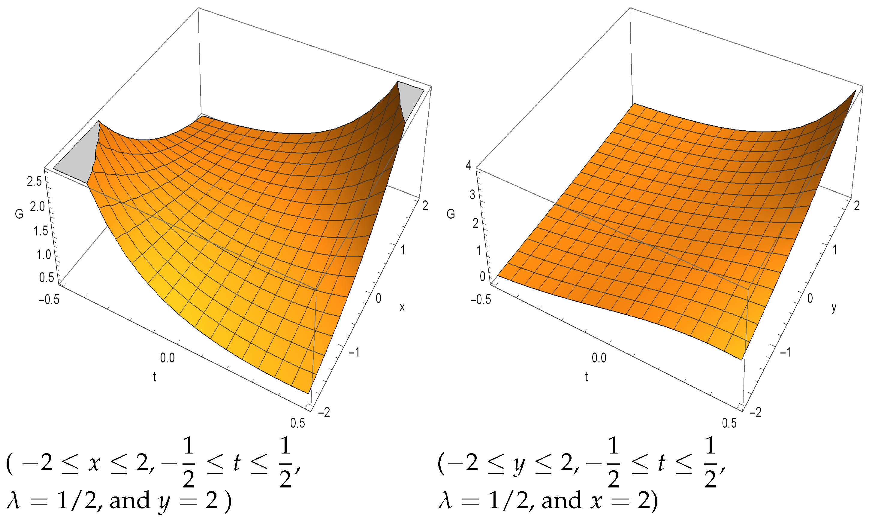
Figure 1.
The surface for the solution = 0.

Figure 2.
Roots of .

Figure 3.
Stacks of roots of .

Figure 4.
Real roots of , .


Table 1.
Numbers of real and complex roots of .
| Degree | Real Roots | Complex Roots | Real Roots | Complex Roots |
|---|---|---|---|---|
| 1 | 1 | 0 | 1 | 0 |
| 2 | 0 | 2 | 2 | 0 |
| 3 | 1 | 2 | 3 | 0 |
| 4 | 0 | 4 | 4 | 0 |
| 5 | 1 | 4 | 5 | 0 |
| 6 | 0 | 6 | 4 | 2 |
| 7 | 1 | 6 | 5 | 2 |
| 8 | 0 | 8 | 6 | 2 |
| 9 | 1 | 8 | 7 | 2 |
| 10 | 0 | 10 | 6 | 4 |
Table 2.
Approximate roots of .
| Degree n | x |
|---|---|
| 1 | 0 |
| 2 | −1.7656, 2.2656 |
| 3 | −2.7231, 0, 4.2231 |
| 4 | −3.2312, −1.4638, 1.6900, 6.0051 |
| 5 | −3.2515, −2.7036, 0, 3.2853, 7.6698 |
| 6 | −1.2884, 1.4301, 4.8062, 9.2488 |
| 7 | −2.3250, 0, 2.8218, 6.2681, 10.762 |
| 8 | −2.9891, −1.1791, 1.2772, 4.1775, 7.6817, 12.221 |
© 2020 by the authors. Licensee MDPI, Basel, Switzerland. This article is an open access article distributed under the terms and conditions of the Creative Commons Attribution (CC BY) license (http://creativecommons.org/licenses/by/4.0/).
Share and Cite
MDPI and ACS Style
Hwang, K.-W.; Ryoo, C.S. Some Identities Involving Two-Variable Partially Degenerate Hermite Polynomials Induced from Differential Equations and Structure of Their Roots. Mathematics 2020, 8, 632. https://doi.org/10.3390/math8040632
AMA Style
Hwang K-W, Ryoo CS. Some Identities Involving Two-Variable Partially Degenerate Hermite Polynomials Induced from Differential Equations and Structure of Their Roots. Mathematics. 2020; 8(4):632. https://doi.org/10.3390/math8040632
Chicago/Turabian StyleHwang, Kyung-Won, and Cheon Seoung Ryoo. 2020. "Some Identities Involving Two-Variable Partially Degenerate Hermite Polynomials Induced from Differential Equations and Structure of Their Roots" Mathematics 8, no. 4: 632. https://doi.org/10.3390/math8040632
Note that from the first issue of 2016, this journal uses article numbers instead of page numbers. See further details here.