On the Advent of Fractional Calculus in Econophysics via Continuous-Time Random Walk

Department of Physics and Astronomy, University of Bologna, & The National Institute of Nuclear Physics (INFN), Via Irnerio 46, I-40126 Bologna, Italy
Mathematics 2020, 8(4), 641; https://doi.org/10.3390/math8040641
Submission received: 30 March 2020
/
Revised: 16 April 2020
/
Accepted: 18 April 2020
/
Published: 21 April 2020
(This article belongs to the Special Issue Mathematical Economics: Application of Fractional Calculus)
Abstract
:In this survey article, at first, the author describes how he was involved in the late 1990s on Econophysics, considered in those times an emerging science. Inside a group of colleagues the methods of the Fractional Calculus were developed to deal with the continuous-time random walks adopted to model the tick-by-tick dynamics of financial markets Then, the analytical results of this approach are presented pointing out the relevance of the Mittag-Leffler function. The consistence of the theoretical analysis is validated with fitting the survival probability for certain futures (BUND and BTP) traded in 1997 at LIFFE, London. Most of the theoretical and numerical results (including figures) reported in this paper were presented by the author at the first Nikkei symposium on Econophysics, held in Tokyo on November 2000 under the title “Empirical Science of Financial Fluctuations” on behalf of his colleagues and published by Springer. The author acknowledges Springer for the license permission of re-using this material.
1. Introduction
As we read from Wikipedia [1], “Econophysics is a heterodox interdisciplinary research field, applying theories and methods originally developed by physicists in order to solve problems in economics, usually those including uncertainty or stochastic processes and nonlinear dynamics. Some of its application to the study of financial markets has also been termed statistical finance referring to its roots in statistical physics”. Here we stress that the problems dealt with in Econophysics are essentially devoted to statistical finance. The first book on Econophysics was by R. N. Mantegna and H. E. Stanley in 2000 [2], followed by a number of books including that by Bouchaud and Potters [3].
The importance of random walks in finance has been known since the seminal work of Bachelier [4] which was completed at the end of the XIXth century, more than a hundred years ago. The ideas of Bachelier were further carried out and improved by many scholars see, for example, Mandelbrot [5], Cootner [6], Samuelson [7], Black and Scholes [8], Merton [9], Mantegna and Stanley [2], Bouchaud and Potters [3].
The term “Econophysics” was coined by H. Eugene Stanley (Boston University) to describe a number of papers written by physicists (including his Ph.D. and Post-Doc students) in the problems of stock and other markets. The inaugural meeting on Econophysics was organized in July 1997 in Budapest by János Kertész and Imre Kondor but the book of proceedings edited by them to be published with the impressive title Econophysics, an Emerging Science was surprisingly cancelled by the publisher Kluwer during the checking of galley proofs.
The author of this paper was alerted on this conference in Budapest from a national newspaper so he was able to get an invitation to present his current research on Lévy stable distributions with his former student Ph.D. Paolo Paradisi and his colleague, the late Professor Rudolf Gorenflo. Indeed, the author was impressed by the derivation of Lévy distributions as fundamental solutions of a space fractional diffusion equation so generalizing the well known Gaussian distribution and the Brownian motion. However, because of the sad end of the book of Budapest proceedings, this paper was not published, but later submitted as an E-print in arXiv, see [10].
Then, after the author’s seminar stable distributions held in Rome, at the University “La Sapienza”, he was approached by Dr. Enrico Scalas of the University of Alessandria (Italy) on the possibility of collaborating with him and his student Marco Raberto and Prof. Rudolf Gorenflo on applications of methods of Fractional Calculus in Econophyscs. As a matter of fact, Enrico Scalas was the director of our group (in Italian called as “Il Regista”, taking inspiration from directing movies) being expert of finance. So a collaboration started inside our group after an introduction paper by Scalas et al. in Physica A, see Reference [11], followed by a series of papers, see Mainardi et al. [12], Gorenflo et al. [13], Raberto et al. [14]. In these papers, the authors have argued that “the continuous-time random walk (CTRW) model, formerly introduced in Statistical Mechanics by Montroll and Weiss [15], can provide a phenomenological description of tick-by-tick dynamics in financial markets” and they have discussed some applications concerning “high frequency exchanges of bond futures”. A particular mention is given to the paper by Mainardi et al. [16], being presented by the author under invitation of the organizer H. Takayasu at an international conference on Econophysics held in Tokyo, November 2000.
Later, other papers were published by our group, see References [17,18] to summarize our approach to CTRW via fractional master equations. Furthermore, Scalas published papers on the relevance of Fractional Calculus in dealing with CTRW in Econophysics, see, for example, Reference [19] and chapters in the book authored by Baleanu et al., see Reference [20,21].
The purpose of this paper is to survey our phenomenological theory of tick-by-tick dynamics in financial markets, based on the continuous-time random walk (CTRW) model, by pointing out the relevance of Fractional Calculus and of the Mittag-Leffler function, a special function almost unknown in those times. Nowadays the Mittag-Leffler function has hundreds citations and a treatise on the functions of the Mittag-Leffler type has been published in 2014 by Gorenflo et al. [22], of which a second enlarged edition will hopefully appear in 2020.
The body of our paper is essentially based on the above references and on the conferences and seminars that anybody of our group could give by invitation in several Institutions spread in the world. In particular, most of the the theoretical and numerical results reported in this paper were presented by the author at the first Nikkei symposium on Econophysics, held in Tokyo on November 2000 under the title “Empirical Science of Financial Fluctuations” on behalf of his colleagues. published in the Springer volume edited by Takayasu [16].
Our survey-article is divided as follows: Section 2 is devoted to revisit the theoretical framework of the CTRW model. We provide the most appropriate form for the general master equation, which is expected to govern the evolution of the probability density for non-local and non-Markovian processes. In Section 3 we propose a master equation containing a time derivative of fractional order to characterize non-Markovian processes with long memory. In this respect, we outline the central role played by the Mittag-Leffler function which exhibits an algebraic tail consistent with such processes. Section 4 is devoted to explain how the CTRW model can be used in describing the financial time series of the log-prices of an asset, for which the time interval between two consecutive transactions varies stochastically. In particular we test the theoretical predictions on the survival-time probability against empirical market data. The empirical analysis concerns high-frequency prices time series of German and Italian bond futures. Finally, in Section 5, we draw the main conclusions. For the sake of convenience, the Appendix A introduces in a simple way the correct notion of time derivative of fractional order.
2. The CTRW Model in Statistical Physics
We recall that the CTRW model leads to the general problem of computing the probability density function (pdf) ( ) of finding, at position x at time t, a particle (the walker) which performs instantaneous random jumps at random instants (), where We denote by the (so-called) waiting times. As usual, it is assumed that the particle is located at for which means We denote by the joint probability density for jumps and waiting times.
The CTRW is generally defined through the requirement that the and are independent identically distributed (i.i.d.) random variables with ’s independent of each other, so that we have the factorization which implies The marginal probability densities w and are called jump pdf and waiting-time pdf, respectively.
We now provide further details on the densities in order to derive their relation with the pdf
The jump pdf represents the for transition of the walker from a point x to a point so it is also called the transition . The waiting-time represents the that a step is taken at the instant after the previous one that happened at the instant so it is also called the pausing-time . Therefore, the probability that is equal to The probability that a given waiting interval is greater or equal to will be denoted by which is defined in terms of by
We note that represents the probability that at least one jump is taken at some instant in the interval , hence is the probability that the walker is sitting in x at least during the time interval of duration after a jump. Recalling that we also note that represents the so called survival probability, namely the probability of finding the walker at the initial position until time instant
Now, only based upon the previous probabilistic arguments, we can derive the evolution equation for the pdf that we shall call the master equation of the CTRW. In fact, we are led to write
where we recognize the role of the survival probability and of the ’s The first term in the RHS of Equation (2) expresses the persistence (whose strength decreases with increasing time) of the initial position . The second term (a spatio-temporal convolution) gives the contribution to from the walker sitting in point at instant jumping to point x just at instant after stopping (or waiting) time Furthermore, as a check for the correctness of Equation (2) we can easily verify that for all and and for all
Originally the master equation was derived by Montroll and Weiss in 1965, see [15], recurring to the tools of the Fourier-Laplace transforms. These authors showed that the Fourier-Laplace transform of satisfies a characteristic equation, now called the Montroll-Weiss equation, which reads
Here, we have adopted the following standard notation for the generic Fourier and Laplace transforms:
where () and () are sufficiently well-behaved functions of their arguments. It is straightforward to verify the equivalence between the Equations (2) and (3) by recalling the well-known properties of the Fourier and Laplace transforms with respect to the space and time convolution.
Hereafter, we present an alternative form to Equation (2), formerly proposed by Mainardi et al. [12], which involves the first time derivative of (along with an additional auxiliary function), so that the resulting equation can be interpreted as an evolution equation of Fokker-Planck-Kolmogorov type. To this purpose, we re-write Equation (3) as
where
Then our master equation reads
where the “auxiliary” function being defined through its Laplace transform in Equation (5), is such that We remind the reader that Equation (6), combined with the initial condition is equivalent to Equation (4), and then its solution represents the Green function or the fundamental solution of the Cauchy problem for Equation (6).
From Equation (6) we recognize the role of as a “memory function”. As a consequence, the CTRW turns out to be in general a non-Markovian process. However, the process is “memoryless”, namely “Markovian” if (and only if) the above memory function degenerates into a delta function (multiplied by a certain positive constant) so that and may only differ by a multiplying positive constant. By appropriate choice of the unit of time we assume so In this case we derive
Then Equation (6) reduces to
This is up to a change of the unit of time (which means multiplication of the RHS by a positive constant), the most general master equation for a Markovian CTRW; it is usually called the Kolmogorov-Feller equation.
3. The Time-Fractional Master Equation with “Long-Memory”
Let us now consider “long-memory” processes, namely non-Markovian processes characterized by a memory function exhibiting a power-law time decay. To this purpose a natural choice is
Thus, is a weakly singular function that, in the limiting case reduces to according to the formal representation of the Dirac generalized function,
As a consequence of the choice (9), we see that (in this peculiar non-Markovian situation) our master equation (6) contains a time fractional derivative. In fact, by inserting into Equation (4) the Laplace transform of we get
so that the resulting Equation (6) can be written as
where is the pseudo-differential operator explicitly defined in the Appendix, that we call the Caputo fractional derivative of order Thus Equation (11) can be considered as the time-fractional generalization of Equation (8) and consequently can be called the time-fractional Kolmogorov-Feller equation.
Our choice for implies peculiar forms for the functions and that generalize the exponential behaviour (7) of the Markovian case. In fact, working in the Laplace domain we get from (5) and (9)
from which by inversion we obtain for
where denotes an entire transcendental function, known as the Mittag-Leffler function of order defined in the complex plane by the power series
For detailed information on the Mittag-Leffler-type functions and their Laplace transforms the reader may consult e.g., the books [22,23] and the articles [24,25].
Hereafter, we find it convenient to summarize the features of the functions and most relevant for our purposes. We begin to quote their series expansions and asymptotic representations:
and
In the limit for we recover the exponential functions of the Markovian case. We note that for both functions , , even if losing their exponential decay by exhibiting power-law tails for large times, keep the “completely monotonic” character. Complete monotonicity of the functions , , , means:
or equivalently, their representability as (real) Laplace transforms of non-negative functions. It may be instructive to note that for sufficiently small times exhibits a behaviour similar to that of a stretched exponential; in fact we have
4. The CTRW Model in Statistical Finance
The price dynamics in financial markets can be mapped onto a random walk whose properties are studied in continuous, rather than discrete, time, see, for example [9]. As a matter of fact, there are various ways in which to embed a random walk in continuous time. Here, we shall base our approach on the CTRW discussed in Section 2, in which time intervals between successive steps are i.i.d. random variables.
Let denote the price of an asset or the value of an index at time t. In finance, returns rather than prices are considered. For this reason, in the following we shall take into account the variable , that is the logarithm of the price. Indeed, for a small price variation , the return and the logarithmic return virtually coincide. The statistical physicist will recognize in x the position of a random walker jumping in one dimension. Thus, in the following, we shall use the language and the notations of Section 2.
In financial markets, prices are fixed when demand and offer meet and a transaction occurs. In this case, we say that a trade takes place. As a consequence, not only prices but also waiting times between two consecutive transactions can be modelled as random variables. In agreement with the assumptions of Section 2, we consider the returns as i.i.d random variables with pdf and the waiting times as i.i.d. random variables with pdf In real processes of financial markets this independence hypothesis may not strictly hold for their duration or not be verified at all. Therefore, it may be considered with caution.
In the following, we limit ourselves to investigate the consistency of the long-memory process analyzed in Section 3 with respect to the empirical data concerning exchanges of certain financial derivatives. We have considered the waiting time distributions of certain futures traded at LIFFE in 1997 and estimated the corresponding empirical survival probabilities. LIFFE stands for London International Financial Futures (and Options) Exchange. It is a London-based derivative market; for further information, see http://www.liffe.com. Futures are derivative contracts in which a party agrees to sell and the other party to buy a fixed amount of an underlying asset at a given price and at a future delivery date.
As underlying assets, we have chosen German and Italian Government bonds, called BUND and BTP respectively, for both of which the delivery dates are June and September 1997. BUND and BTP (Buoni del Tesoro Poliennali) are respectively the German and Italian word for BOND (middle and long term Government bonds with fixed interest rate). Usually, for a future with a certain maturity, transactions begin 4 or 5 months before the delivery date. At the beginning, there are few trades a day, but closer to the delivery there may be more than 1000 transactions a day. For each maturity, the total number of transactions is greater than 160,000. Hence, these types of financial instruments are particularly interesting for the analysis of the waiting times distributions between consecutive transactions.
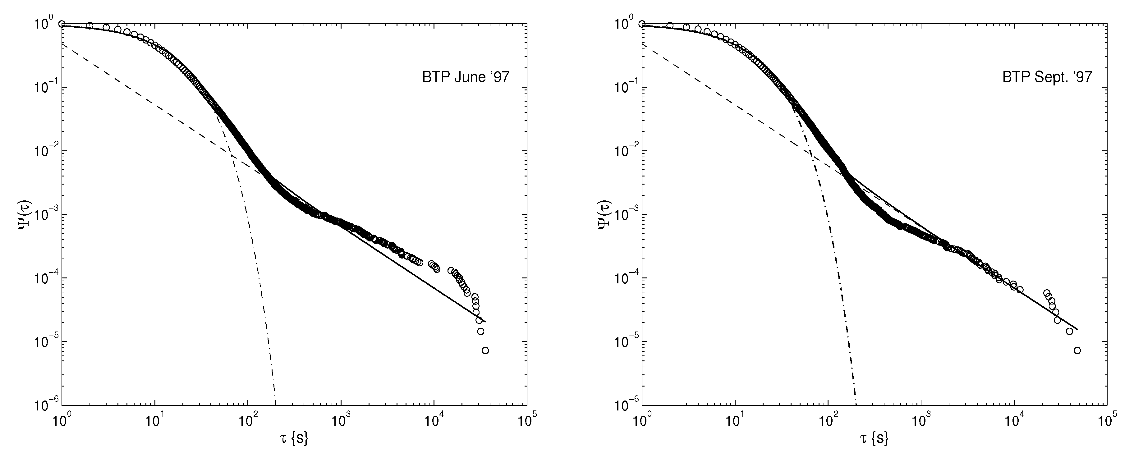
In Figure 1 and Figure 2 we plot for the four cases (June and September delivery dates for BUND and BTP). The circles refer to market data and represent the probability of a waiting time greater than the abscissa . We have determined about 500–600 values of for in the interval between 1 s and 50,000 s, neglecting the intervals of market closure. The solid line is a two-parameter fit obtained by using the Mittag-Leffler type function
where is the index of the Mittag-Leffler function and is a time-scale factor, depending on the time unit. The dash-dotted line is the stretched exponential function see the RHS of Equation (18), whereas the dashed line is the power law function , see the RHS of the second Equation in (15), noting that The Mittag-Leffler function well interpolates between these two limiting behaviours—the stretched exponential for small times, and the power law for large ones.
As regards the BUND futures we can summarize as follows. For the June delivery date we get an index and a scale factor whereas, for the September delivery date, we have and The fits in the plots of Figure 1 have a reduced chi square . As regards the BTP futures we can summarize as follows. For both the June and September delivery dates we get the same index and the same scale factor The fits in the plots of Figure 2 have a reduced chi square .
To the possible objection that, in all four cases here treated, does not differ significantly from 1 and so the process still could be Markovian, we answer that then we would have and the graph of would look completely different for sufficiently long times.
5. Conclusions
In this paper, we have reviewed our phenomenological theory of tick-by-tick dynamics in financial markets, based on the continuous-time random walk (CTRW) model. The theory can take into account the possibility of the non-Markovian character of financial time series by means of a generalized master equation with a time fractional derivative. We have presented predictions of the behaviour of the waiting-time probability density by introducing a special function of Mittag-Leffler type whose decay interpolates from a stretched exponential at small times to a power-law for long times. This function has been successfully applied in the empirical analysis of high-frequency prices time series of German and Italian bond futures. We may note the common behaviour of the survival probabilities found from the trading of the above assets. This might be corroborated or not in other cases.
Funding
This research received no external funding.
Acknowledgments
The author is grateful to V. Tarasov for having invited him to survey the former approach to Econophysics using the methods of Fractional Calculus that the author has shared with the colleagues R. Gorenflo, M. Raberto and E. Scalas. The research activity of the author has been carried out in the framework of the activities of the National Group of Mathematical Physics (GNFM, INdAM).
Conflicts of Interest
The author declares no conflict of interest.
Appendix A. The Caputo Fractional Derivative
For the sake of convenience of the reader here we present an introduction to the Caputo fractional derivative starting from its representation in the Laplace domain and pointing out its difference with respect to the standard Riemann-Liouville fractional derivative. So doing, we avoid the subtleties lying in the inversion of fractional integrals. If is a (sufficiently well-behaved) function with Laplace transform we have
if we define
We can also write
References
- Wikipedia. Econophysics. 2020. Available online: https://en.wikipedia.org/wiki/Econophysics (accessed on 17 April 2020).
- Mantegna, R.N.; Stanley, H.E. An Introduction to Econophysics; Cambridge University Press: Cambridge, UK, 2000. [Google Scholar]
- Bouchaud, J.-P.; Potters, M. Theory of Financial Risk: From Statistical Physics to Risk Management; Cambridge Univ. Press: Cambridge, UK, 2000. [Google Scholar]
- Bachelier, L.J.B. Théorie de la Speculation. Ann. École Norm. Supérieure 1900, 17, 21–86, Reprinted by Editions Jaques: Gabay, Paris, 1995. (English Translation with Editor’s Notes in The Random Character of Stock Market Prices, pp. 17–78). [Google Scholar] [CrossRef]
- Mandelbrot, B.B. The variation of certain speculative prices. J. Bus. 1963, 36, 394–419, (Reprinted in The Random Character of Stock Market Prices, pp. 307–332). [Google Scholar] [CrossRef]
- Cootner, P.H. (Ed.) The Random Character of Stock Market Prices; MIT Press: Cambridge, MA, USA, 1964. [Google Scholar]
- Samuelson, P.A. Rational theory of warrant pricing. Ind. Manag. Rev. 1965, 6, 13–31. [Google Scholar]
- Black, F.; Scholes, M. The pricing of options and corporate liabilities. J. Polit. Econ. 1973, 81, 637–659. [Google Scholar] [CrossRef] [Green Version]
- Merton, R.C. Continuous Time Finance; Blackwell: Cambridge, MA, USA, 1990. [Google Scholar]
- Mainardi, F.; Paradisi, P.; Gorenflo, R. Probability distributions generated by fractional diffusion equations. In Proceedings of the Workshop on Econophysics, Budapest, Hungary, 21–27 July 1997; Invited Lecture; Department of Physics: Bologna, Italy, January 1998; pp. ii+39. [Google Scholar]
- Scalas, E.; Gorenflo, R.; Mainardi, F. Fractional calculus and continuous-time finance. Physica A 2000, 284, 376–384. [Google Scholar] [CrossRef] [Green Version]
- Mainardi, F.; Raberto, M.; Gorenflo, R.; Scalas, E. Fractional calculus and continuous-time finance II: The waiting-time distribution. Physica A 2000, 287, 468–481. [Google Scholar] [CrossRef] [Green Version]
- Gorenflo, R.; Mainardi, F.; Scalas, E.; Raberto, R. Fractional calculus and continuous-time finance III: The diffusion limit. In Mathematical Finance; Kohlmann, M., Tang, S., Eds.; Birkhäuser Verlag: Basel, Switzerland; Boston, MA, USA; Berlin, Germany, 2001; pp. 171–180. [Google Scholar]
- Raberto, M.; Scalas, E.; Mainardi, F. Waiting-times and returns in high-frequency financial data: An empirical study. Physica A 2001, 314, 751–757. [Google Scholar] [CrossRef] [Green Version]
- Montroll, E.W.; Weiss, G.H. Random walks on lattices, II. J. Math. Phys. 1965, 6, 167–181. [Google Scholar] [CrossRef]
- Mainardi, F.; Raberto, M.; Scalas, E.; Gorenflo, R. Survival probability of LIFFE bond futures via the Mittag-Leffler function. In Empirical Science of Financial Fluctuations; Takayasu, H., Ed.; Springer: Tokyo, Japan, 2002; pp. 195–206. [Google Scholar]
- Gorenflo, R.; Mainardi, F. Fractional diffusion processes: Probability distributions and continuous-time random walk. In Processes with Long-Range Correlations; Rangarajan, G., Ding, M., Eds.; Springer: Berlin, Germany, 2003; pp. 148–166. [Google Scholar]
- Scalas, E.; Gorenflo, R.; Mainardi, F. Uncoupled continuous-time random walks: Solution and limiting behavior of the master equation. Phys. Rev. E 2004, 69, 011107. [Google Scholar] [CrossRef] [PubMed] [Green Version]
- Scalas, E. The application of continuous-time random walks in finance and economics. Physica A 2006, 362, 225–239. [Google Scholar] [CrossRef]
- Scalas, E. Continuous-Time Random Walks and Fractional Diffusion Models. In Fractional Calculus: Models and Numerical Methods, 2nd ed.; Baleanu, D., Diethelm, K., Scalas, E., Trujillo, J.J., Eds.; World Scientific: Singapore, 2017; Chapter 6; pp. 291–320, (1st Edition, 2012). [Google Scholar]
- Scalas, E. Applications of Continuous-Time Random Walks. In Fractional Calculus: Models and Numerical Methods, 2nd ed.; Baleanu, D., Diethelm, K., Scalas, E., Trujillo, J.J., Eds.; World Scientific: Singapore, 2017; Chapter 7; pp. 321–344, (1st Edition, 2012). [Google Scholar]
- Gorenflo, R.; Kilbas, A.A.; Mainardi, F.; Rogosin, S.V. Mittag-Leffler Functions. Related Topics and Applications; Springer Monographs in Mathematics; Springer: Berlin, Germany, 2014; p. XIV-443. ISBN 978-3-662-43929-6. [Google Scholar]
- Erdélyi, A.; Magnus, W.; Oberhettinger, F.; Tricomi, F.G. Higher Transcendental Functions; McGraw-Hill: New York, NY, USA, 1955; Volume 3, pp. 206–227. [Google Scholar]
- Gorenflo, R.; Mainardi, F. Fractional calculus, integral and differential equations of fractional order. In Fractals and Fractional Calculus in Continuum Mechanics; CISM Lecture Notes; Carpinteri, A., Mainardi, F., Eds.; Springer: Wien, Austria; New York, NY, USA, 1997; Volume 378, pp. 223–276. [Google Scholar]
- Mainardi, F.; Gorenflo, R. On Mittag-Leffler type functions in fractional evolution processes. J. Comput. Appl. Math. 2000, 118, 283–299. [Google Scholar] [CrossRef] [Green Version]
- Samko, S.G.; Kilbas, A.A.; Marichev, O.I. Fractional Integrals and Derivatives, Theory and Applications; (Translated from the Russian (Nauka i Tekhnika, Minsk, 1987)); Gordon and Breach: Amsterdam, The Netherlands, 1993. [Google Scholar]
- Podlubny, I. Fractional Differential Equations; Academic Press: San Diego, CA, USA, 1999. [Google Scholar]
Figure 1.
Survival probability for BUND futures with delivery date: June 1997 (left) September 1997 (right). The Mittag-Leffler function (solid line) is compared with the stretched exponential (dash-dotted line) and the power (dashed line) functions: {} (left); {)} (right).
Figure 1.
Survival probability for BUND futures with delivery date: June 1997 (left) September 1997 (right). The Mittag-Leffler function (solid line) is compared with the stretched exponential (dash-dotted line) and the power (dashed line) functions: {} (left); {)} (right).

Figure 2.
Survival probability for BTP futures with delivery date: June 1997 (left) September 1997 (right). The Mittag-Leffler function (solid line) is compared with the stretched exponential (dash-dotted line) and the power (dashed line) functions: {} (left); {)} (right).
Figure 2.
Survival probability for BTP futures with delivery date: June 1997 (left) September 1997 (right). The Mittag-Leffler function (solid line) is compared with the stretched exponential (dash-dotted line) and the power (dashed line) functions: {} (left); {)} (right).

© 2020 by the author. Licensee MDPI, Basel, Switzerland. This article is an open access article distributed under the terms and conditions of the Creative Commons Attribution (CC BY) license (http://creativecommons.org/licenses/by/4.0/).
Share and Cite
MDPI and ACS Style
Mainardi, F. On the Advent of Fractional Calculus in Econophysics via Continuous-Time Random Walk. Mathematics 2020, 8, 641. https://doi.org/10.3390/math8040641
AMA Style
Mainardi F. On the Advent of Fractional Calculus in Econophysics via Continuous-Time Random Walk. Mathematics. 2020; 8(4):641. https://doi.org/10.3390/math8040641
Chicago/Turabian StyleMainardi, Francesco. 2020. "On the Advent of Fractional Calculus in Econophysics via Continuous-Time Random Walk" Mathematics 8, no. 4: 641. https://doi.org/10.3390/math8040641
Note that from the first issue of 2016, this journal uses article numbers instead of page numbers. See further details here.