A Novel Algorithm with Multiple Consumer Demand Response Priorities in Residential Unbalanced LV Electricity Distribution Networks

Abstract

Demand Side Management (DSM) is becoming necessary in residential electricity distribution networks where local electricity trading is implemented. Amongst the DSM tools, Demand Response (DR) is used to engage the consumers in the market by voluntary disconnection of high consumption receptors at peak demand hours. As a part of the transition to Smart Grids, there is a high interest in DR applications for residential consumers connected in intelligent grids which allow remote controlling of receptors by electricity distribution system operators and Home Energy Management Systems (HEMS) at consumer homes. This paper proposes a novel algorithm for multi-objective DR optimization in low voltage distribution networks with unbalanced loads, that takes into account individual consumer comfort settings and several technical objectives for the network operator. Phase load balancing, two approaches for minimum comfort disturbance of consumers and two alternatives for network loss reduction are proposed as objectives for DR. An original and faster method of replacing load flow calculations in the evaluation of the feasible solutions is proposed. A case study demonstrates the capabilities of the algorithm.

1. Introduction

The shift from the old structure of the government-controlled electricity generation and tariff system existing in many parts of the world to the deregulated market model has aimed to incentivize innovation in the field, to lower the electricity cost, and to create new services for the consumers. In parallel, the climate change concerns have raised the need to push forward the generation of ‘clean’ electricity from renewable and non-polluting primary sources, which led to the necessity of creating the regulatory environment and tools required to enable wholesale and small-scale trading of electricity generated in large or small green electricity sources [1]. The proliferation of small-scale distributed generation sources in Medium Voltage (MV) and Low Voltage (LV) distribution networks changed the operation conditions and management requirements of these networks, that must now integrate new technologies and management procedures. Distribution System Operators (DSO) need to convert the existing supply infrastructure into smart grids with enhanced monitoring and communication capabilities. Consumers have to turn to HEMS in order to manage IoT devices and to sell the surplus of local generation to the market.

The convergence of these developments leads to the need of developing new categories of market services at the MV and LV electricity distribution level. One of these new advances is the Demand Side Management (DSM). A specific DSM branch is Demand Response (DR), that allows DSO utilities or microgrid operators to manage the consumer load in specific time intervals in order to alleviate high network loading at peak consumer hours or in other special operating conditions. Essentially, DR consists of an agreement between a coordinating entity (network operator or market aggregator) and a set of individual consumers which allows the former to demand or act unilaterally for reducing the consumers’ load, in exchange for other benefits for the consumer. As described in [2], several types of DR exist, broadly classified in two main categories—incentive-based and tariff-based. The existing DR initiatives have focused on the industrial sector, mostly in developed countries. However, the residential sector is becoming lately a major focus for DR.

The literature offers a broad spectrum of research carried out in this field. Regarding the methodologies and hypotheses used for DR, multi-objective optimization is the preferred choice. Papers [3,4] use a multi-objective approach, carried out applying Load Management (LM) strategies and evolutionary methods. Here, the problem combines DR and real-time price estimation. Two objectives are considered -the minimization of the daily cost of active power and the minimization of customer dissatisfaction. Furthermore, it is expected to obtain similar and more flattened consumer demand profiles with sporadic peaks and a more secure and reliable network operation and control. In paper [5], a multi-objective theoretical optimization methodology for the energy payments is proposed, based on the interpretation of the correlation between price flexibility and probabilistic consumption, which considers stochastic load models. The investigation aims to improve the ability to accommodate wind production uncertainty. Moreover, the correlation between the quantity of DR programs and their efficiency is realized by actively engaging end-users in power networks.

Another multi-objective DR approach is used in [6], where three players are considered—the distribution network, the end-users, and the aggregator who intermediates between them. Using the Artificial Immune Algorithm (AIA), a Pareto optimal variable set is reached. Next, an optimal solution is chosen, so that all the aforementioned actors can profit: The network operator can decrease the generation cost; the DR aggregator can obtain an advantage by granting DR assistance; the end-users can save funds. A two-stage stochastic simulation is used in [7] to minimize two objective functions (operation cost and air pollution). The suggested approach records the energy and resources produced by generating systems and active loads. The independent network operator receives the power quantity disconnected via DR and its recommended price from the DR providers. The DR price is then shaped by the price elasticity of the load demand. The multi-objective DR model is based on the Augmented Epsilon Constraint (AEC) method. Other authors propose multi-objective DR programs performed at the same time with the generation and storage units dispatch [8].

In [9], a Multi-Rate Model Predictive Control (MPC) is used to maximize the consumption from local PV panels generation so that the electricity drawn from the network and the need for DR to be minimized. Consequently, [10] considers a multi-objective Genetic Algorithm (GA) optimization method to help both the utilities optimize their DR by minimizing the network operation cost and maximizing consumer earnings.

In other works, the DR process is performed managing gap-filling to create loads during off-peak intervals [11]; peak cutting to decrease loads at peak intervals [12] or load shifting, which mixes gap loading and peak cutting actions [13]. The DR schedules are separated into reliability or market-based DR applications [14]. At the same time, the aforementioned articles describe DR goals compared with day ahead optimization, hour ahead optimization, system peak reduction, local balancing, on-line control, small scale distribution sources optimization, and basic RES integration. The DR programs can be applied, as it is demonstrated in [15], based on the improvement of data-driven Machine Learning (ML) with fixed and flexible load prediction models for a retail structure.

The papers [16,17] extend the residential DR model to more elaborate and realistic in three-phase unbalanced distribution networks using Modified Particle Swarm Optimization (MPSO) or Direct Load Control (DLC) methods. Here, multi-objective optimization problems are considered to solve DR for residential users, developing a Pareto Optimal Demand Response (PODR) algorithm [18], or using the Non-Dominated Sorting Firefly Algorithm (NDSFA) in [19]. The mixed problem of utility selection and DR supervision in a smart grid consisting of many electricity utilities and various clients is investigated in [20] with a reinforcement learning and Game-Theoretic Technique (GTT). In [21,22,23], particular approaches for the optimization of the PV-battery system of houses reducing both energy costs and DR activities based on Mixed-Integer Linear Programming (MILP) are presented. In other initial assumptions, the authors from [24,25] propose an efficient objective function to decrease the cost of microgrid operation considering large-scale plug-in electric vehicles and Renewable Energy Sources (RES). Here, the advantage of end-users is modelled by using incentives for including electric vehicle charging in DR programs.

This paper proposes a novel algorithm for DR optimization usable in radial three-phase, four-wire LV electricity distribution networks that supply one-phase residential consumers. Such algorithms were proposed before, in papers such as [9,16,17]. However, in these existing approaches the operation state of the network is assessed using load flow computations, which are time-costly, especially for networks with larger sizes [26,27,28], and they are limited to proposing two objective functions.

Table 1. Comparison between the literature and the proposed approach.

Number of Reference	Phase Load Balancing	Individual Consumer Disturbance	Overall Consumer Disturbance	Power Losses without Load Flow Computation	Used Algorithm/Method	Network Type—no. of Consumers	Objective Function
[3,4]	No	Yes	Yes	No	NSGA-II	Test—1 cons.	OF1+OF2
[5]	Yes	No	Yes	No	PSO	Real—151 cons.	OF1+OF4
[6]	No	No	Yes	No	AIA	Test—1 cons.	OF1+OF5
[7]	No	Yes	No	No	AEC	IEEE—30	OF1+OF6
[8]	No	Yes	Yes	No	NSGA-II	IEEE24—30 cons.	OF1+OF2
[9]	Yes	No	No	No	MPC	Test—25 cons.	OF4+OF5
[10]	No	Yes	Yes	No	GA	Test—1 cons.	OF1+OF5
[15]	No	No	No	No	ML	Test—1 cons.	OF1+OF3
[16]	No	Yes	No	No	MPSO	Real—77 cons.	OF3+OF7
[17]	Yes	No	No	No	DLC	IEEE10—15 cons.	OF1+OF4
[18]	No	No	Yes	No	PODR	Test—400 cons.	OF1+OF8
[19]	No	No	Yes	No	NDSFA	IEEE—30, Real—101 cons.	OF1+OF5
[20]	No	Yes	Yes	No	GTT	Test—100 cons.	OF1+OF5
[21]	Yes	Yes	Yes	No	MILP	Test—20 cons.	OF1+OF9
[22]	Yes	Yes	Yes	No	MILP	IEEE—RBTS.	OF1+OF9
[23]	Yes	Yes	Yes	No	MILP	Test—1 cons.	OF1+OF9
[24]	No	Yes	Yes	No	GA	Test microgrid.	OF1+OF5
[25]	Yes	No	No	No	MPC	Test—1 cons.	OF4+OF5
[27]	No	No	No	No	GA-ANN	Test—3 cons.	OF5+OF8
The proposed approach	Yes	Yes	Yes	Yes	MOPSO	Real—176 cons.	OF1+OF2+OF3+OF4+OF5+OF8

provides a comparison between the capabilities of the proposed approach with regard to the literature review discussed above. The notations from the last column, for the objective functions considered in the optimization, are: OF1—minimize the operation cost; OF2—minimize the consumer dissatisfaction; OF3—active power loss minimization; OF4—maximize the electricity consumption satisfaction; OF5—maximize the net revenue for consumers; OF6—air pollutants emission minimization; OF7—minimize the compensation costs of voltage management; OF8—maximize the load factor; OF9—minimize the curtailment weights. The type and number of consumers of the networks used in the case studies are given in the seventh column of the table, for comparison with the approach used in the paper. The cases with one consumer denote that the DR is performed at the household level.

The proposed method offers more flexibility and ease of use, combining several features present in the literature review summarized in Table 1 and giving the choice of using more objective functions for optimization. The main characteristics of the proposed algorithm are:

• The use of the Multi-Objective Particle Swarm Optimization (MOPSO) for identifying the optimal solutions
• The solutions are provided as Pareto frontiers for optimizing two conflicting objectives
• In the initial implementation, the users can choose between five possible objective functions, belonging to two distinct categories (technical and user comfort):

  ○

  Phase load balancing at the supply substation level

  ○

  The minimization of individual consumer disturbance caused by DR

  ○

  The minimization of overall consumer disturbance caused by DR

  ○

  An original, faster method for active power loss minimization

  ○

  A load-flow based method for active power loss minimization (for comparison purposes).

Except for the optional load flow method, the other objective functions require the knowledge of minimal data about the electrical network, that can be grouped in a matrix consisting of eight lines and a number of columns equal to the number of consumers existing in the network. The formulation of each DR objective has a simple mathematical model, which contributes to a fast execution time for the algorithm. The specific formulation of the input data allows the possibility of implementing individual consumer DR segmentation on independent levels according to comfort preferences. The optimization is based on the MOPSO algorithm because it allows an easy definition of other objectives for DR and has fast execution times. The results of the case study, performed on a real LV distribution system, show that the algorithm performs as expected for all the pairs of objective functions tested, and that the proposed loss minimization method combines increased computation speed and good accuracy when compared with the classic load flow approach.

The rest of the paper is structured as follows: Section 2, Materials and Methods, provides the detailed description of the proposed DR objectives, with their differences and practical usability, together with the mathematical model for each objective, followed by the general structure of the MOPSO algorithm in which they are used; Section 3 presents the electrical network used for testing the algorithm and the results of the case study; Section 4, Discussion, presents the advantages and limitations of the proposed approach, ending with the future research directions envisioned by the authors.

2. Materials and Methods

The proposed multi-objective DR optimization algorithm is aiming to provide to DSO and other entities a tool for enabling DR initiatives in distribution systems. As a working hypothesis, it is considered the case of low voltage four-wire distribution networks that supply mostly one-phase consumers connected through one-phase branchings to three-phase feeders. As it would be the case in real conditions, it is also considered that only a fraction of the total number of consumers connected in the network will participate in the DR program, due to technical (i.e., too low consumption) or personal (i.e., unwillingness) reasons. Out of the participating consumers, some can be equipped with HEMS systems which allow them to set custom DR levels to be accessed by the algorithm, that are modelling consumer preferences or comfort levels. Such systems are widely studied in the literature, one example being the HEMS proposed in [29].

When the utility initiates a DR request, given as a power amount P_dec to be disconnected from the entire network, specified in kW or percent fraction from the total current network load, the algorithm has the task of distributing the power quantity requested between the consumers in the network such as a pair of two conflicting objectives to be fulfilled. The user (DSO) can choose from five available objective functions:

• F1—Phase load balancing. The aim of this objective is to disconnect individual loads from the network so that phase load balancing is to be achieved on all three phases at the substation which supplies the entire LV network, or, in other words, to minimize the differences between the phase power flows at the supply point.
• F2—The minimization of individual consumer disturbance. This goal aims to distribute the load disconnection between the available consumers such as each individual consumer will have a minimal comfort reduction because of its participation to DR.
• F3—The minimization of overall consumer disturbance, that will ensure that the DR request will affect the minimal number of consumers.
• F4—Active power losses minimization in the network. Here, the aim is to disconnect loads ensuring that the operation of the network with the remaining load will result in minimal active power losses.

For this objective, an original approach is implemented, which prioritizes for disconnection the loads located near the farthest end of the distribution feeders and the loads where the power disconnected during the DR event is maximum. This approach aims to prevent the use of time-consuming load flow algorithms for computing the losses and to minimize the amount of input data used in calculations, as it does not require the knowledge of the network configuration or of the electrical parameters of its branches.

• F5—Active power losses minimization in the network. In this approach, the active power losses are computed using a load flow algorithm. This is the method most used in the literature, and is implemented for comparison with the approach proposed for F4.

All the fitness functions are taking into consideration the deviation between the total power disconnected in the DR event and the DR target set by the utility, P_dec, which needs to be fulfilled as close as possible.

A more detailed description and the mathematical models for F1–F5 will follow in Section 2.3.

The results are provided as Pareto frontiers, which are built using the Multi-Objective Particle Swarm Optimization (MOPSO) [30], described briefly in the following subsection.

2.1. The Multi-Objective Particle Swarm Optimization Algorithm

The MOPSO algorithm, proposed in 2002 by C.A. Coello and M.S. Lechuga for solving Pareto-conditioned problems, is an extension for multi-objective optimization problems of the well-known Particle Swarm Optimization (PSO) algorithm [31]. Its basic flowchart for two objective functions is provided in Figure 1. Compared to the original PSO [32,33], the MOPSO evaluates the solutions, that are encoded as numeric vectors, for two conflicting objective functions, and accommodates the necessary modifications to keep the multiple solutions that make a Pareto frontier, using an external archive. The population members (particles) change their speed and position for the next iteration (p^(it+1)) according to the classic PSO equations:

$$v_{}^{(it)}=w\cdot v_{}^{\begin{array}{l}\\ (it-1)\end{array}}+2\cdot rn{d}_1\cdot (p_{best}^{(it)}-p_{crt}^{(it)})+2\cdot rn{d}_2\cdot (leade{r}_{}^{(it)}-p_{}^{(it)})$$

(1)

$$p_{}{}^{(it+1)}=p_{}{}^{(it)}+v_{}{}^{(it)}$$

(2)

In Equations (1) and (2), v^(it) and v_j^(it-1) are the speed of the particle in the previous (it-1) and current (it) iteration, rnd₁ and rnd₂ are vectors of random numbers, p_best^(it) and p^(it) are the best personal and the current position of the particle, leader^(it) is the position of the leader in iteration it, and w is an inertia coefficient decreasing over the iteration count to progressively narrow the search space around the current optimal solution.

After updating its position, each particle is subjected to a mutation procedure for increasing diversity inside the population. Moreover, since the optimal solution is not unique, the leader is selected for each particle from the external archive. Any mutation and selection procedure applied in the literature for evolutionary algorithms can be used for this purpose.

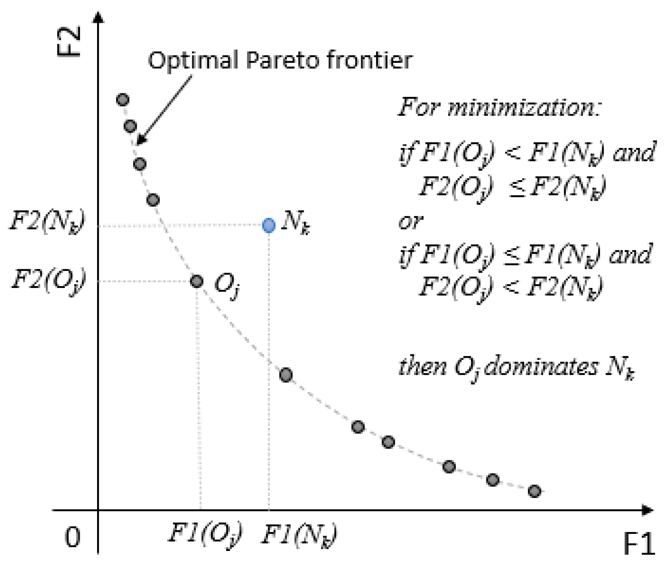
In the Pareto frontier of optimal solutions (external archive) found by the algorithm are allowed only non-dominated solutions. The conditions required for non-dominance when solving minimization problems are depicted in Figure 2. Usually, a fixed maximum number of solutions NS_max is allowed in the Pareto frontier. For enforcing this constraint while encouraging a uniform distribution of solutions across the entire length of the frontier, the solutions from the most crowded sections are pruned with specific procedures, so that the number of solutions that are found at any time in the frontier, NS, is lower than NS_max.

Several algorithms from the literature can be used for multi-criterial optimization, as the survey from Table 1 shows. The choice for the MOPSO considered several advantages. The algorithm was previously used with proven results in various engineering fields such as industrial manufacturing [34], photovoltaic panel design [35], water reservoir operation [36] or optimal dispatch of electricity generation [37]. Compared with other classic or metaheuristic optimization algorithms, MOPSO has a simpler mathematical model, which makes its more accessible and flexible for industry specialists looking to adopt new management tools with minimal training and costs. The simple mathematical model minimizes the computation time, improving the speed of the optimization and of the decision making process. Moreover, the PSO algorithm was previously used by the authors for solving single-objective DR optimization, in [38].

2.2. The Input Data Required and the Encoding of a Solution

If load flow calculations are not used, the proposed algorithm requires minimal input data for performing the DR optimization. For an electrical network with NN buses or nodes, NC consumers and NB branches, one input matrix DataIN is required, with the structure presented in

Table 2. The input data required by the algorithm—the structure of matrix DataIN.

Consumer 1	Consumer 2	Consumer i	Consumer NC
index1	index2	indexi	indexNC
phase1	phase2	phasei	phaseNC
dist1	dist2	disti	distNC
PC1	PC2	PCi	PCNC
PDR,1,1	PDR,2,1	PDR,i,1	PDR,NC,1
PDR,1,2	PDR,2,2	PDR,i,2	PDR,NC,2
PDR,1,3	PDR,2,3	PDR,i,3	PDR,NC,3
PDR,1,4	PDR,2,4	PDR,i,4	PDR,NC,4

, where, for any consumer i, i = 1..NC, the following notations are used: index_i—consumer index, phase_i—the connection phase (1, 2, 3 or 0, denoting phases a, b, c, and three-phase consumer, respectively), dist_i—the distance measured between the consumer and the supply source (MV/LV substation), PC_i—the power demand of the consumer, in kW, in the interval of analysis and in the absence of DR load reduction, P_DR,i,1—P_DR,i,4—the power which the consumer is willing to disconnect in a DR event. The DR availability of any consumer, denoted as maxDR_i, is described by a maximum of four levels of comfort that can be accessed in their decreasing order (indexes 4 to 1) by the utility in order to fulfill its DR objective. The consumers that do not participate to DR will not use any of these levels and will not be considered for optimization. The consumers with at least one active level are candidates for DR. They submit their maximum disconnection levels which they make available for load reduction, and the algorithm selects the actual number of levels that will be used for optimization. The consumers with one active level can also account for clients who do not have HEMS implemented, but wish to participate in the DR program. Thus, the real number of consumers from the network participating in the DR program is NC_DR ≤ NC.

A particle that describes a solution of the MOPSO algorithm is a vector of integer numbers of size NC_DR:

P=p_j∈ℤ ^{1x NCDR}, pj ∈ [0,4]

(3)

and has the structure described in

Table 3. The encoding used by a particle in the MOPSO algorithm.

Consumer 1	Consumer 2	Consumer j	Consumer NCDR
level1	level2	levelj	levelNCDR

, where level_j is the highest available DR level remaining in use after optimization (i.e., the power available at levels level_j +1 to maxDR_j is disconnected during the DR event).

An example of writing the matrix DataIN and interpreting a solution p_j is given in Appendix A, at the end of the paper.

2.3. The Objective Functions Used for Optimization

The MOPSO algorithm can be used to build the Pareto frontiers for two out of five conflicting objective functions, previously defined as F1–F5. It should be noted that the objective function pool can be easily extended, with minimal changes to the algorithm, required only by possible new input data required by the new objective functions. The mathematical models of the objective functions are designed to be simple and intuitive, for minimizing the computation time and increasing the practical usability. The information contained in the input data is minimal and well known by network operators.

2.3.1. The Objective Function F1—Maximum Substation Phase Load Balancing (SPB)

The optimal operation conditions of three-phase electricity distribution systems require that the power flows on the three phases should be as close as possible to equal, on all the feeders that supply consumers. A substantial deviation from this constraint can lead to two undesired effects:

• If the phase demand is unbalanced, power flows on the neutral wire increase, leading to supplementary power losses.
• On the phase(s) with the highest load, supplementary power losses and higher voltage drops will occur, increasing with the length of the feeders and the load.

The normal operation conditions of these networks are usually with unbalanced phase load, because of the continuous variation of the demand and unoptimized phase connection of the consumers. Optimized DR can help alleviate the imbalance by finding the best candidates for DR, from the available pool, such as the demand remaining unaffected to be more balanced on the phases.

The algorithm used in the paper proposes that DR should be requested from the consumers in such a way that power is disconnected predominantly from the phases with the highest load, in order to equalize the power flows on the three phases. The balancing procedure used for DR optimization consists of several steps.

F1.1. For each DR consumer j, read the DR request (the actual DR operation level which will remain active in the DR interval, as requested by the utility), according to the current particle p. This information allows the computation of the power disconnected from each consumer and phase.

actualDR_j = p_j

(4)

where j = 1..NC_DR.

F1.2. Find the total active power which will be disconnected from each consumer, PD_j, and subtract it from the total power consumption of the consumer, in order to determine the power requirement PCj remaining on each phase, after DR is applied.

$$P{D}_j={\displaystyle \sum _{\begin{array}{l}k=actualD{R}_j+1\\ actualD{R}_j\ne 0\end{array}}^{\max D{R}_j}{P}_{DR,j,k}},j=1..N{C}_{DR}$$

(5)

$$P{C}_j=P{C}_j-P{D}_j,j=1..N{C}_{DR}$$

(6)

F1.3. Using the consumer phase allocation phase_i, i = 1..NC, compute the sum of demand P_ph on each phase ph:

$$P_{ph}={\displaystyle \sum _{phas{e}_i=ph}^{}P{C}_i},i=1..NC,ph,phas{e}_i=1,2,3$$

(7)

F1.4. Compute the standard deviation of active power flows on the three phases of the network at the LV busbar. A low standard deviation of the three phase power flows (P_a, P_b, P_c) is a result of close values of these three quantities.

$$a1=stdev(P_a,P_b,P_c)$$

(8)

F1.5. Compute the difference between the total load disconnected in the DR event and the target set by the utility, because the phase balance must be achieved with the constraint that the amount of power disconnected via DR matches the target set by the network operator, P_dec:

$$b=abs(P_{dec}-{\displaystyle \sum _{j=1}^{N{C}_{DR}}P{D}_j})$$

(9)

F1.6. Compute the objective function F1 for particle p as a combination of the considered targets, balancing and amount of disconnected power, where a high deviation of the latter is seen as a penalizing factor for the first:

$$F1=a1+b/P_{dec}\cdot 100$$

(10)

The objective of the optimization is to find the solutions with minimal imbalance which adhere to the target quantity of power disconnected set by the network operator:

$$\underset{s=1..NS}{\min }(F{1}_s)$$

(11)

2.3.2. The Objective Function F2—The Minimization of the Individual Consumer Disturbance (ICD)

One of the deterrents that would make the residential consumers avoid subscribing into DR initiatives proposed by utilities is the expected loss of comfort generated by the need to limit their electricity demand during the DR hours, which often will coincide to evening times, when the home power demand is at its peak. To alleviate this problem, the utility could consider to distribute its total DR requirement between the consumers such as the comfort level of each consumer would be minimally affected. This is similar to disconnecting power from each consumer on fewer DR levels as possible.

The computation of this objective function requires the following steps:

F2.1. For each DR consumer j, read the DR request actualDR_j, with Equation (4), according to the current particle p.

F2.2. Determine the number of affected DR levels, for each consumer j:

$$a{2}_j=maxD{R}_j-actualD{R}_j,j=1..N{C}_{DR}$$

(12)

F2.3. For affected levels greater than 1, simulate a penalizing factor. A high number of affected levels for a consumer means a greater loss of comfort. The higher the number of levels affected for an individual consumer, the higher the penalizing factor should be, increasing the value of a2. A low value of a2 means that, generally, consumers need to disconnect a minimal number of DR levels.

$$a{2}_{}={\displaystyle \sum _{\begin{array}{l}j=1\\ a{2}_j\ne 0\end{array}}^{N{C}_{DR}}a{2}_j^2}$$

(13)

F2.4. Compute the difference between the total load disconnected in the DR event and the target set by the utility, with (9).

F2.5. Compute the objective function F2 for particle p as the average value of a2 for each DR consumer in the network, penalized by the deviation between the actual amount of disconnected power and the target set by the network operator:

$$F2=a2/N{C}_{DR}+b/P_{dec}\cdot 100$$

(14)

The two factors are averaged for the number of DR consumers and DR target for obtaining similar fitness values in networks with a different number of consumers and different DR targets set by the network operators.

The objective of the optimization is to find the solutions with the lowest value of F2:

$$\underset{s=1..NS}{\min }(F{2}_s)$$

(15)

2.3.3. The Objective Function F3—The Minimization of the Overall Consumer Disturbance (OCD)

Another goal of an electricity utility when using DR in the network can be to minimize the number of affected consumers. Such an approach would ensure that the majority of consumers will not have to reduce their demand, and their comfort will not be affected. However, the comfort loss cost would be transferred to the consumers which will need to reduce their load, as they would be forced to minimize their demand. While this objective could be considered unfeasible to pursue on its own in real operation conditions, because of the high stress placed on the affected consumers, it becomes of interest in the context of Pareto optimality, when another objective such as power loss minimization is sought.

This objective is implemented in the MOPSO algorithm by searching for solutions that use the maximum number of DR levels for individual consumers. The following steps are used:

F3.1. For each DR consumer j, compute the DR request actualDR_j, with Equation (4).

F3.2. Determine the number of affected DR levels, for each consumer j, with (12):

$$a{3}_j=maxD{R}_j-actualD{R}_j,j=1..N{C}_{DR}$$

(16)

F3.3. Count the number of zero elements computed in the previous step, that should be maximized, because this is the number of consumers which do not disconnect power in the DR event and will not suffer from loss of comfort:

$$a3=\mathrm{count}(a{3}_j=0),j=1..N{C}_{DR}$$

(17)

F3.4. Compute the difference between the total load disconnected in the DR event and the target set by the utility, with (10).

F3.5. Compute the objective function F3 for particle p, as the inverse of coefficient a3 averaged over the number of DR consumers, taking into account, as for F1 and F2, the compliance with the target of the network operator:

$$F3=1/(a3\ast N{C}_{DR})+b/P_{dec}\cdot 100$$

(18)

The objective of the optimization is to find the solutions with a minimal number of affected DR levels for each individual consumer:

$$\underset{s=1..NS}{\min }(F{3}_s)$$

(19)

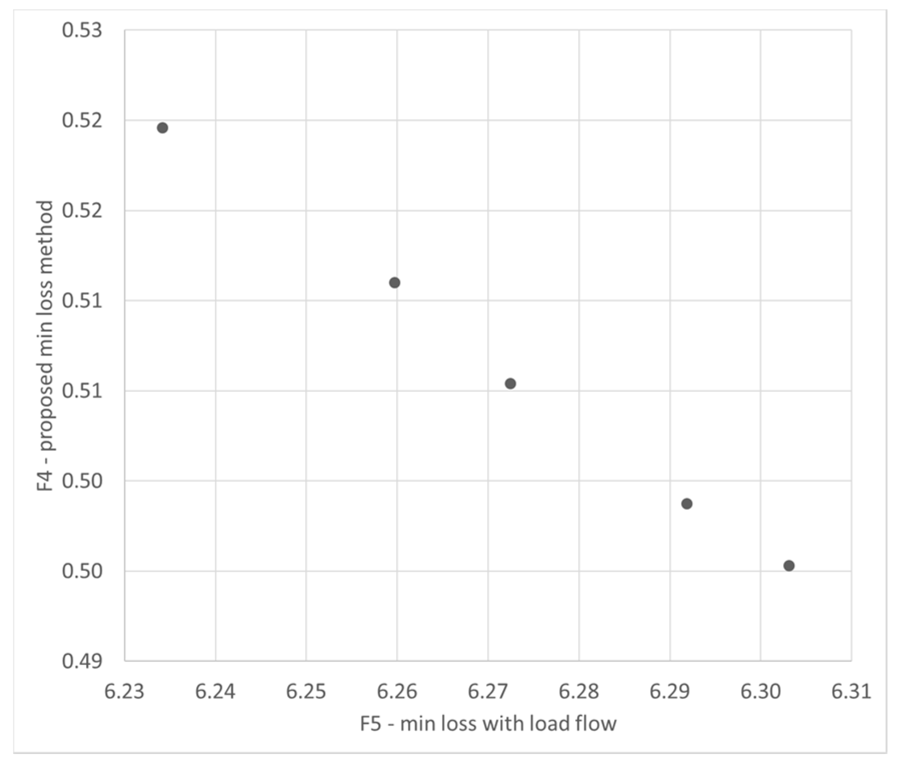
2.3.4. The Objective Function F4—The Active Power Loss Minimization Using the Simplified Method Proposed in the Paper (SMP)

One of the main objectives of the DSO utilities is to operate their networks with minimal active power losses. At medium and high voltage levels, this goal can be achieved by optimally setting the operational configuration of the equipment or by optimal generation dispatch. At LV level, load management is one of the few measures available that do not necessitate supplementary investment costs. As it has been shown in the literature survey, this objective has been approached in the literature mainly using load flow calculations to determine the losses associated with the optimal DR solutions. While offering the best precision, this method is time consuming and requires the knowledge of the operating configuration of the LV network, together with the electrical parameters of all its elements, which are not always known in detail.

This paper proposes a much simpler approach to finding DR solutions which lead to network operation with minimal losses. Its advantages, with a marginally precision loss trade-off, are:

• Significantly reduced computation time when compared to load flow methods, which makes the approach more attractive for implementation in real-time applications.
• The knowledge of network configuration and electrical parameters is not needed.

The proposed method combines two principles widely used for loss minimization in radial electricity distribution networks, by encouraging DR load reduction for two categories of loads:

• Consumers located far from the supply point
• Consumers with a high demand and number of DR levels.

The associated objective function for this approach is using several steps:

F4.1. For each DR consumer j, compute the DR request actualDRj, with Equation (4).

F4.2. Find PD_j and PC_j, for each DR consumer, with Equations (5) and (6).

F4.3. For each DR consumer j, find the network length separating it from the source, dist_j, as given in the input matrix DataIN.

F4.4. Compute the total distance separating the consumers affected by the DR request from the source—the distance factor, the first component of the objective function:

$$a41={\displaystyle \sum _{\begin{array}{c}j=1\\ actualD{R}_j\ne 0\end{array}}^{N{C}_{DR}}dis{t}_j}$$

(20)

F4.5. Compute the total power disconnected from the consumers in the DR event—the maximum load disconnection factor, the second component of the objective function:

$$a42={\displaystyle \sum _{j=1}^{N{C}_{DR}}P{D}_j}$$

(21)

F4.6. Compute the difference between the total load disconnected in the DR event and the target set by the utility, with Equation (9).

F4.7. Compute function F4 for particle p combining the values for the three components (distance, high individual load, DR target):

$$F4=a41/N{C}_{DR}+a42/P_{net}+b/P_{dec}\cdot 100$$

(22)

where P_net is the power demand of the LV network before the DR event:

$$P_{net}={\displaystyle \sum _{i=1}^{NC}DataIN(4,i)}$$

(23)

The objective of the optimization is to find the solutions with the minimal value for F4:

$$\underset{s=1..NS}{\min }(F{4}_s)$$

(24)

2.3.5. Objective Function F5—Active Power Loss Minimization Using a Load Flow Method (LFM)

For the assessment of the performance of the load minimization method proposed in the previous subsection, a graph-theory based load flow method for radial distribution networks was implemented. Its steps follow.

F5.1 Using the data from the input matrix DataIN, compute the bus loads PC_bus in [kW] and find the bus currents [A] using the bus rated voltage U_n,bus [kV]:

$$P{C}_{bus}={\displaystyle \sum _{\begin{array}{l}i=1\\ i=bus\end{array}}^{NC}DataIn(4,i)},bus=\mathrm{1...}NB$$

(25)

$$I_{bus}=P{C}_{bus}/U_{n,bus},bus=\mathrm{1...}NB$$

(26)

F5.2. Using the incidence matrix A written for the distribution network and the bus currents vector I_b = I_bus ∈ ℝ ^{1x NC}, find the branch currents vector I_br, given in [A]:

$$I_{br}=-inv(A)\cdot I_b$$

(27)

F5.3. If I_branch are elements from I_br, compute the branch losses for the entire network in [kW]:

$$\Delta P_{branch}=R_{a,branch}\cdot I_{branch}^2\cdot K_{branch}\cdot {10}^{-3}[\mathrm{kW}]$$

(28)

$$\Delta P={\displaystyle \sum _{branch=1}^{NB}}\Delta P_{branch}$$

(29)

In Equation (28), K_branch is a coefficient that accounts for the loss increase due to the phase load imbalance, computed with:

$$K_{branch}=CU{F}_{branch}\cdot \left(1+1.5\cdot \frac{R_{n,branch}}{R_{a,branch}}\right)-1.5\cdot \frac{R_{n,branch}}{R_{a,branch}}$$

(30)

where CUF_branch is the current imbalance factor computed for each branch with:

$$CU{F}_{branch}=\frac{1}{3}\cdot \left[{\left(\frac{I_{branch,a}}{I_{branch,abc}^{average}}\right)}^2+{\left(\frac{I_{branch,b}}{I_{branch,abc}^{average}}\right)}^2+{\left(\frac{I_{branch,c}}{I_{branch,abc}^{average}}\right)}^2\right]$$

(31)

In (30) and (31), I_branch,a, I_branch,b, I_branch,c are the branch currents on phases a, b, and c; I_br,abc ^average are the average current on phases a, b, and c, and R_a,branch, R_n,branch are the resistance of the active phase and neutral wire of each branch, measured in [Ω]. The compliance with the DR target set by the network operator is also considered, as for F1-F4.

The objective of the optimization is to find the solutions with minimal losses:

$$\underset{s=1..NS}{\min }(F{5}_s)=\underset{s=1..NS}{\min }(\Delta P_s)$$

(32)

Each objective function is called a subroutine as functions F1 and F2, as seen in Figure 1. As an example, in Algorithm 1 the code used for the objective function F4, SMP is provided. Similar algorithms can be written for the other objective functions. In Algorithm 1, indexDR is a vector of size NC_DR containing the indexes of the DR consumers in the network, determined using the first row from DataIN and the list of known DR clients from the network, pop is the population of the MOPSO algorithm, and NP is its size.

Algorithm 1. The subroutine used to encode the calculation steps for the objective function F4—the simplified loss minimization method proposed in the paper.

1. Read the input data: pop, NP, DataIN, NCDR, indexDR, Pnet, Pdec, maxDR.

for each particle p from the population

2. Initialize a41 = 0, a42 = 0, a43 = 0.

3. for each DR client k, k =1..NCDR

3.1. Read the DR availability of client k: ptemp = DataIN(5:8,indexDR(k))

3.2. Compute the power disconnected from client k, according to particle p:

Lim1 = p(k) + 1

Lim2 = maxDR(k)

PD = sum(ptemp(Lim1:Lim2))

3.3. Update the value of the power disconnected in the network: a43 = a43 + PD(k)

3.4. if PD > 0, read the distance separating client k from the supply point:

d = DataIN(2,indexDR(k))

3.5. Update the first two components of the objective function:

a41 = a41 + dist

a42 = a42 + PD

4. Compute the three components of the objective function:

a41 = a41 / NCDR

a42 = a42 / Pnet

a43 = abs (Pdec – a43) / (Pdec) *100

5. Compute the value of the objective function F4 for the current particle:

F4 = a41 + a42 + a43

Return F4, a41, a42, a43 for all the particles

3. Case Study

The algorithm aims to provide a flexible tool for DSOs and local microgrid operators who choose to implement DR programs for optimizing the operation of their network. For demonstrating its performances, a low voltage distribution network with real measured data and corresponding to the residential consumer profile mostly expected to adhere to DR (individual houses from a residential neighborhood) was chosen. The five objective functions were grouped in pairs and the optimization algorithm was run. The results show that the choice of objectives leads to different DR requirements from the consumers. The newly proposed objective function F4, aimed to replace time-consuming load flow computation, shows good adequacy.

3.1. The LV Network Used in the Case Study

The DR algorithm described in Section 2 was tested using a real LV, four-wire electricity distribution network, its one-line diagram being shown in Figure 3. The network supplies only one-phase residential consumers through Overhead Lines (OHL) feeders mounted on poles. In Figure 3, the black bullets represent pole indices, and the arrows point to the number of consumers supplied at each pole.

The feeders are four-wire, while the consumer branchings are two-wire (active phase and neutral conductors). The supplied area consists of mainly one- and two-storied houses located at the outskirts of a small sized town. The main technical characteristics of this network are provided in

Table 4. The main characteristics of the LV network used in the case study.

Characteristic	Value
Number of poles	36
Network length (4-wire feeders)	1512 m
Network length (4-wire feeders and 2-wire branchings)	7600 m
Wire type—4-wire feeders	3 × 50 + 50 mm2, overhead cable
Wire type—2-wire branchings	25 + 16 mm2, overhead cable

.

The consumers supplied by the network can be classified, based on their peak demand, as in

Table 5. Consumer categories based on their peak power demand and maximum number of demand response (DR) levels used for each category.

Consumer Peak Power	Count	DR Levels Used in the Case Study
<0.5 kW	92	0
>0.5 and ≤0.7 kW	28	1
>0.7 and ≤1 kW	41	2
>1 and ≤1.5 kW	8	3
>1.5 kW	7	4

. As described in Section 2, only the consumers with a peak consumption greater than a given limit (0.5 kW in this case) were included in the DR pool. In the time interval used for analysis, this approach resulted in 40.5 kW of power available for DR, from a maximum number of 84 consumers, at a total network power consumption of 116.6 kW. It should be noted that the LV substation transformer which supplies the network has a rated power of 180 kVA.

3.2. Algorithm Setup and Results

The algorithm was run for a maximum of 1000 generations, with 70 individuals in the population. The Pareto frontiers obtained for different pairs of objective functions are presented in Figure 4, Figure 5, Figure 6, Figure 7 and Figure 8 and

Table 6. Fitness functions for the pair F5-F2

Solution No.	F5 LFM	F2 ICD
1	6.379	1.795
2	6.427	1.545
3	6.465	1.425
4	6.564	1.354
5	6.616	1.354
6	6.637	1.342
7 (best ICD)	7.276	1.295

,

Table 7. Fitness functions for the pair F1–F2.

Solution No.	F1 MPB	F2 ICD
1	6.959	1.687
2	6.997	1.628
3	7.132	1.568
4	7.139	1.556
5	7.504	1.485
6	7.657	1.473
7	7.711	1.414
8	7.845	1.390
9	7.978	1.330
10	8.457	1.306

,

Table 8. Fitness functions for the pair F1–F3.

Solution No.	F1 MPB	F3 OCD
1 (best MPB)	5.763	0.443
2	5.992	0.419
3	6.183	0.400
4	6.602	0.395
5 (best OCD)	6.952	0.388

,

Table 9. Fitness functions for the pair F5–F4.

Solution No.	F5 LFM	F4 SMP
1 (worst SMP)	6.234	0.520
2	6.260	0.511
3	6.272	0.505
4	6.292	0.499
5 (best SMP)	6.303	0.495

and

Table 10. Fitness functions for the pair F1–F5.

Solution No.	F1 MPB	F5 LFM
1	5.836	6.103
2 (best LFM)	5.992	6.033

.

In Appendix B,

Table A1. The matrix DataIN written for the LV distribution network depicted in Figure A1.

Consumer, Indexi	1	2	3	4	5	6	7	8	9	10	11	12
connection phase, phasei	1	2	1	2	0	1	1	3	1	3	3	2
distance to source [m], disti	40	40	80	120	120	160	240	240	240	240	280	280
consumption [kW], PCi	0.2	1.3	5.1	0.8	0.8	0.3	1.1	0.7	0.5	0.7	1.7	3.2
DR level 1, [kW], PDR,i,1	0	0.2	0.5	0	0.3	0	0.3	0.2	0	0	0.3	0.5
DR level 2, [kW], PDR,i,1	0	0.5	0.5	0	0	0	0.4	0	0	0	0.5	1.2
DR level 3, [kW], PDR,i,1	0	0	0.7	0	0	0	0	0	0	0	0.3	0
DR level 4, [kW], PDR,i,1	0	0	0.7	0	0	0	0	0	0	0	0	0

, the solutions obtained by the algorithm corresponding to the best values obtained for each objective function are given, compared to the initial solution (no DR applied). For comparison purposes, the synthetic data (functions F1–F5, network losses and unbalance, number of affected consumers) are provided in

Table 11. Detailed results for relevant solutions obtained by the algorithm—objective functions.

	Case	Fitness	F1, MPB	F2, ICD	F3, OCD	F4, SMP	F5, LFM
solution	initial, no DR	N/A	111.253	100.000	1.000	100.000	108.642
	best MPB	F1 = 5.763	5.763	1.854	0.443	0.489	6.396
	best ICD	F2 = 1.295	9.718	1.295	0.752	0.550	7.276
	best OCD	F3 = 0.388	6.952	2.396	0.388	0.973	7.114
	best SMP	F4 = 0.495	6.005	1.806	0.443	0.495	6.303
	worst SMP	F4 = 0.520	7.111	1.652	0.526	0.520	6.234
	best LFM	F4 = 6.033	5.992	1.699	0.586	0.532	6.033

and

Table 12. Detailed results for relevant solutions obtained by the algorithm—network results.

Case	Stdev (Pa, Pb, Pc)	Loss, kW	Loss, %	Loss Error, %	DR Mismatch, kW	No. of Consumers Affected by DR
initial, no DR	11.25	10.08	8.64	32.99%	20.25	0
best MPB	5.52	5.93	6.15	5.85%	0.05	37
best ICD	9.47	6.78	7.03	17.64%	0.05	63
best OCD	6.21	6.15	6.37	9.11%	0.15	32
best SMP	5.76	5.83	6.06	4.46%	0.05	37
worst SMP	6.86	5.77	5.99	3.34%	0.05	44
best LFM	5.74	5.57	5.79	Ref.	0.05	49

.

Several aspects can be observed from the data presented above. First of all, the number of solutions in the Pareto frontier is small for any pair of objective functions chosen for optimization. This can be attributed to the fact that, as an analysis on the matrix DataIN shows, there are multiple solutions that can involve different consumers chosen for DR, resulting in the same value of the fitness function. As an example, disconnecting 0.2 kW alt DR level 2 from consumers 146 or 167 would have the same effect on the value of objective function F1 (MPB, Maximum Phase Balancing at substation level) or F3 (OCD, Overall Consumer Disturbance). Due to its size, the matrix DataIN is provided only as a Supplementary File with the paper.

The objective function F1 (MPB) has the same effect on power losses as F4 (SMP) and F5 (LFM), because phase balancing leads to lower current flows on the neutral wire and lower maximum phase current flows, which both result in lower active power losses. This is why it can be observed that the pair F1–F5 has the lowest number of solutions, because objectives F1 and F5 are not always conflicting (Table 10, Figure 8). The same can be observed for pair F5-F4 (LFM, SMP), where the extremities of the Pareto frontier are very narrow (between 6.23 and 6.3 for F5 and 0.49–0.52 for F4). If the load flow method is used as reference, the error in loss calculation is of 3.34% for the proposed method, while the loss reduction achieved by DR is of 33% (best LFM).

The values from Figure 7 and Table 9 show that the proposed method can be a good tradeoff between speed and accuracy. While the results regarding the active power loss in the network are marginally worse than those obtained using the load flow method (F5) (5.99–6.06%, as opposed to 5.79%, and compared to the reference no DR case of 8.64%), they are better than the active power losses obtained after balancing with the objective function F1—6.15%, as seen in Table 12. The proposed method, SMP (F4), has also the advantage of better speed. In MATLAB, on a Ryzen 5 1600X 6-core machine with 16 GB of RAM, the time cost of running an iteration of the algorithm with the function pair F3–F4 is 0.214 s, while running the function pair F3–F5 takes 0.654 s, which makes the proposed method three times faster than the classic graph theory-based load flow. Running the algorithm with the settings specified in Section 3.2 (1000 iterations, population size 70, Ryzen 5 PC with MATLAB), the average running times for combinations of F1 to F4 varied between 37 s (pair F1–F4) and 33 s (pair F2–F3). If the time-costly load flow objective is used, the time can amount up to 235 s (pair F1–F5). These times can be further improved by using distributed, parallel computation amongst the available computing cores and also depend on the number of DR consumers in the network. In the paper, parallel computation was disabled and the number of DR consumers (thus the length of the MOPSO particles processed) is high, at 84, for simulating the use of hardware and network situations that are common in real operation conditions.

Regarding the robustness characteristics of the proposed method, the computation times obtained above, the literature comparison from Table 1, and the network data from Table 4 show that the proposed methods are suitable for large size networks, with a high number of consumers. Using as reference the data from [39], the network chosen for the case study is representative for the type of residential consumption currently existing in Europe, and comparing it with the information from Table 1, it is the amongst the largest used, at a length of 1.5 km and a number of DR consumers of 84 out of 176 possible.

Using any of the objective functions F1–F5 leads to reducing the active power losses in the network, because in all the cases DR reduces the network load, but the most significant reductions are obtained using the objective functions F1, F4, or F5, which are mostly technical in nature. The other two objective functions, F2 and F3 are comfort based, aiming to reduce the disturbance for the individual consumers affected by DR (F2) or the number of consumers affected (F3). As Table 12 shows, the number of affected consumers is the largest for F2 and the smallest for F3, a behavior consistent with the sought objective (in order to achieve the same disconnected power amount, a larger number of consumers will be affected less and a smaller number of consumers will be affected more). From

Table A3. Solutions found by the MOPSO-DR algorithm.

		Consumer Index				2	6	7	9	10	11	13	15	16
		no DR				3	2	2	1	2	1	1	3	2
		best MPB		F1 = 5.763		1	1	0	1	2	0	1	0	1
		best ICD		F2 = 1.295		3	1	1	0	1	1	1	2	1
Solution		best OCD		F3= 0.388		0	1	0	1	2	0	1	0	1
		best SMP		F4 = 0.495		3	2	1	1	2	0	1	3	2
		worst SMP		F4 = 0.52		3	2	2	1	2	1	1	2	1
		best LFM		F4 = 6.033		2	2	1	1	2	0	0	2	2
19		20	21	22	24	28	30	32	34	35	36	37	38	40
4		1	1	1	1	2	2	3	1	4	2	1	2	3
1		1	1	0	0	2	2	0	1	0	0	1	1	2
1		1	0	0	1	1	1	3	0	3	1	1	1	3
0		1	1	1	0	2	2	3	1	1	2	1	2	2
0		0	1	1	0	2	2	1	1	0	2	0	1	2
2		0	1	1	0	2	2	1	1	0	2	0	2	3
2		0	1	1	0	2	2	1	0	0	1	1	0	3
44	48	49	53	54	57	58	60	63	64	68	70	71	72	74
2	2	1	2	2	2	1	3	2	4	2	2	4	2	2
1	1	1	0	2	0	1	3	2	0	1	1	3	2	2
1	1	1	1	1	1	1	2	1	3	1	1	2	1	1
0	1	1	2	1	0	1	3	2	1	1	0	4	2	1
1	0	1	0	2	0	1	0	2	2	1	2	2	2	2
2	1	1	2	1	0	1	0	1	2	1	2	1	2	2
2	2	1	0	2	1	1	1	0	1	1	2	3	2	2
2	2	1	2	2	2	1	3	2	4	2	2	4	2	2
75	76	78	80	82	83	85	86	90	92	93	95	99	100	101
1	1	3	1	2	1	2	2	2	2	2	2	2	1	1
1	1	1	1	2	1	0	2	2	0	1	1	0	1	1
1	0	2	1	1	1	1	1	1	1	1	1	1	0	1
1	1	2	1	1	1	0	2	2	2	1	1	2	1	1
1	1	3	1	1	1	0	2	2	1	1	0	2	1	1
1	1	3	1	1	1	0	1	2	1	1	1	1	0	0
1	0	1	0	1	1	2	1	2	2	2	1	2	0	1
102	103	105	106	110	111	112	113	115	116	119	120	121	131	132
2	1	4	1	2	2	2	2	2	2	4	1	3	1	3
0	0	3	1	2	2	2	2	2	2	2	1	3	1	2
1	1	2	0	1	1	1	1	1	1	1	1	2	1	1
1	0	0	1	2	2	2	2	2	2	0	1	3	1	2
1	1	0	1	1	2	0	2	1	1	3	0	3	1	0
2	1	1	1	1	0	0	2	2	1	3	0	2	0	1
1	1	2	0	1	2	1	1	1	2	3	1	3	0	0
139	140	145	146	147	148	149	155	156	165	167	169	172	174	176
2	1	2	2	1	2	4	2	1	1	2	1	2	1	2
2	1	2	2	1	0	1	2	1	1	1	1	2	1	1
1	0	1	1	1	1	3	1	1	0	1	1	1	1	1
2	1	1	2	1	2	0	1	1	1	1	1	2	1	2
1	1	0	2	1	2	3	2	1	1	2	1	2	1	0
1	0	1	2	1	2	1	2	1	1	0	0	1	1	1
1	0	1	1	0	1	0	0	1	0	1	0	2	1	1

, it can be seen that when optimizing with function F3, the algorithm chooses for DR preferentially the consumers with the highest number of DR levels available.

The economic aspects of implementing the DR initiatives in LV residential networks can be viewed from two perspectives. First, there is the effect on the network. Reducing power losses leads to savings in primary energy resources. For the best cases found by the algorithm, losses are reduced via DR with 4.31 kW when using the objective function F4 and 4.51 kW when using the objective function F5. If this value is extrapolated for 365 days and 3 h a day (the peak evening hours), the saving amount to 4.72 and 4.94 MWh of electricity. Their cost can vary according to the primary source. At a reference price of 0.2 EUR/kWh for households, as seen in the EUROSTAT statistics, the yearly savings for this network and DR scenario would be up to 988 EUR.

On the other hand, the consumers agree to participate in DR in exchange for other services or tariff reductions offered by the network operator. These advantages are difficult to quantify, because they can imply both economic and comfort components.

Moreover, for all the fitness functions used, the algorithm complies with the DR limit set by the network operator (20.25 kW) with an error of 0.05 kW determined by the one-decimal load representation on the DR levels. The only exception is the optimal solution found for F3, which is a 0.15 kW error.

4. Discussion

The algorithm presented in the paper can serve DSOs and other entities such as microgrid operators as a tool to test and implement DR services which take into consideration multiple optimization goals, combining technical and user comfort criteria. The higher number of fitness functions that are available in its current implementation give it an advantage over other alternatives from the literature. Furthermore, there is the possibility to include with minimum modifications more types of objectives, as each objective is being implemented as a subroutine called independently.

In real world implementation, the algorithm is, however, dependent on the existence of intelligent grids, capable of two-way communication with the network operator, and intelligent Home Energy Management systems are required to enable the multi-level DR approach. This can be currently considered a limitation in its applicability, until Smart Grids will become more common.

The results of the case study have shown that there is a dependence between the chosen optimization and the results. For instance, the DR requests that give lowest power loss values are not detected by combinations of fitness functions that include user comfort-oriented objectives, which, in turn, lead to solutions with higher than average loss values.

The results from Table 6, Table 7, Table 8, Table 9 and Table 10 suggest also that the algorithm is more likely to find compromise solutions, rather than favoring the cases that belong to the extremities of the Pareto frontier, weighted towards one of the objective functions. Some reasons for these results could be found in the significant length of the particles needing to be optimized by the MOPSO (84 in this case) and in the typical behavior of metaheuristics, which have simpler optimization models, with the tradeoff of finding near-optimal solutions.

The simplified approach to load minimization proposed in the paper, while does not reach the global optimal loss value, shows the advantage of speed coupled with near-optimal results, which can constitute an acceptable compromise for real time or short-term optimization. This objective function can have an advantage over the classical load flow approach in scenarios when network operators prioritize speed in their decision-making processes.

Future research directions envisioned for the algorithm are the testing of other optimization methods such as the NSGA-II for generating the Pareto frontiers, further improvement of the mathematical model of the DR objectives, the extension of the optimization model to include several consecutive DR intervals and the DR rebound, and further expansion of the number of concurrent optimization criteria, by using a many-objective approach such as the NSGA-III algorithm [40].