Numerical Approach of the Equilibrium Solutions of a Global Climate Model

Abstract

We consider a coupled model surface-deep ocean effect, where an Energy Balance Model (EBM) is used for modelling the surface temperature and a two-dimensional heat equation represents the evolution of the temperature of the deep ocean. Although the model under study is based on that proposed by Watts & Morantine (1990), here we consider a modified model that incorporates other processes, such as the nonlinear diffusion and the action of coalbedo, depending on the temperature. The stationary states of the model under study, taking the solar constant as the parameter, are numerically attained. The results of the simulation are depicted in a $\left\{\right(Q,u\left)\right\}$ plot where u is the temperature in the surface and Q is the solar constant. The numerical solution is achieved by means of a finite volume scheme with Weighted Essentially Non-Oscillatory (WENO) reconstruction in space and third order Runge-Kutta scheme, which verifies the Total Variation Diminishing (TVD) property, for time integration. The equilibrium states are accomplished by evolving in time the numerical solution until the stationary solutions are reached. The main novel results of this work concern the numerical obtention of the stationary solutions of both the EBM and the coupled model EBM-deep ocean and the agreement of these results with the theoretically obtained in previous works, where an interval of values of the solar constant Q was obtained with the existence of at least three stationary solutions. In this work, we have numerically obtained more than three stationary solutions for such interval of Q.

1. Introduction

Climate system is very complex and it involves many components and complicate mechanisms. The full behaviour of the climate is something still far to be understood. The pioneering climate Energy Balance Models (EBMs) were introduced by Budyko and Sellers separately (1969) in [1,2], respectively. EBMs are diagnostic models that describe the evolution of the climate for relatively long scales. Several aspects of the mathematical treatment of different versions of climate EBMs have been studied by many authors, such as [3,4,5,6,7], just to name a few of them. In this work, we are concerned with a two-dimensional climate model (latitude-depth), which represents the coupling: mean surface temperature with ocean temperature. It is based on a climate model proposed by Watts and Morantine [8], which is composed of a parabolic equation in a global ocean with a dynamic and diffusive boundary condition, but incorporating additional terms, such as nonlinear diffusion and the coalbedo, depending on the temperature (see [9,10]). Regarding the numerical simulation of this type of climate models, several references can be mentioned, such as [11,12] using finite element methods or [13,14] based on finite volume methods (FVMs). Finite volume methods are very efficient techniques for the numerical approach of the solution of problems governed by balance laws, as those considered in this work. In FVMs, the REA (Reconstruction-Evolution-Averaging) algorithm, see [15], is applied. Thus, this numerical technique involves the computation of integral averages of the solution for each grid cell (also denominated as cell averages) at each time step. Certain reconstruction process is required in order to compute values and gradients from the cell averages where needed. This reconstruction function is usually piecewise polynomial of certain degree, and must be conservative in each one of the control volumes that conform the stencil, so as to keep the conservation properties of the finite volume method. We note that, with the purpose of developing numerical schemes of order greater than one, it is necessary to implement a nonlinear numerical approach, which allows to overcome Godunov’s theorem [16], which states that monotone behavior of a numerical solution cannot be assured for linear finite-difference methods with more than first-order accuracy. As a first approach, second-order accurate schemes can be obtained based on nonlinear piecewise linear reconstruction, such as the minmod method, the Nessyahu-Tadmor scheme, WAF (Weighted Average Flux) scheme, or the MUSCL-Hancock approach (which is second order in space and time), just to mention some possibilities. Complete and detailed descriptions on finite volume techniques can be consulted in [15,17,18]. The first successful attempt to obtain high order monotone numerical schemes are the Essentially Non-Oscillatory (ENO) methods, which were put forward in the pioneering work of Harten, Engquist, Osher, and Chakravarthy in 1987 [19], where the stencil of the reconstruction polynomial is chosen in such a way that it avoids non-physical oscillations in the numerical solution. It is a nonlinear scheme in the sense that it uses known values of the solution in order to select the stencil. Another alternative, widely used nowadays, are the so called Weighted Essentially Non-Oscillatory (WENO) schemes introduced in [20] which, instead of choosing the "smoothest" stencil, as in the ENO approach, a convex combination of all candidate stencils is performed, considering the values taken by certain smoothness indicators, in order to achieve the essentially non-oscillatory property. This WENO procedure is the one implemented in this work to accomplish the high-order nonlinear reconstruction (see, e.g., [21,22,23,24,25] for a detailed description on this technique). Once the reconstruction function is obtained, values of the solution and gradients are attained where needed. In a general case, if we wish to achieve an order of accuracy $(2r-1)$, then we must consider r candidate stencils, each one of them with r cells. A variant of classical WENO approach is the so-called Central WENO (CWENO) scheme [26,27,28,29,30], which makes use of polynomials of different degrees. Other relevant references with different ways to implement WENO methodology can be found in [31,32,33]. With regard to the evolution stage, we remark that we are producing a semi-discrete approach, in which the spatial discretization, performed by means of the FVM, converts the original partial differential equation (PDE) into an ordinary differential equation (ODE). The numerical solution of the ODE requires to implement an ODEs solver. In this work, we have resorted to the third order Runge-Kutta Total Variation Diminishing (RK3-TVD) scheme. Pioneering works on Runge-Kutta TVD methods with different orders of accuracy can be found in [34,35]. The RK3-TVD is a one-step method developed in three stages verifying the remarkable TVD property, which allows for avoiding non-physical oscillations in the numerical solution and it was introduced in the context of second order finite difference schemes by Ami Harten [36]. This property means that being $u_i^n$ the averaged numerical solution for cell i and time $t^n$, it is verified that $TV\left(u_i^n\right)\le TV\left(u_i^{n+1}\right)$, where $TV(·)$ represents the so-called Total Variation, which is given by ${\displaystyle TV\left(u\right)=\sum _i(u_{i+1}-u_i)}$. The aim of this work is to obtain numerically, by means of the finite volume method with WENO reconstruction and RK3-TVD scheme for time integration, the equilibrium states and an approximation of a subset of the bifurcation diagram in a global climate model taking the solar constant as the parameter. We are interested in computing the stationary states of the EBM, without influence of the deep ocean, and also of the coupling EBM-deep ocean. The reason behind the consideration of these two situations is that both cases are relevant in climatic modelling. In the case of EBMs, without ocean effect, they are frequently used in many studies of global climate, see, for instance [3,4,7,37,38] and references therein, as they allow to predict the average surface temperature of the Earth due to incoming solar radiation, emission of radiation, energy absorption, and greenhouse effects, among other phenomena. On the other hand, the inclusion of the ocean effect has an important influence on the temperatures distribution due to the well-known thermostatic effect of the ocean, absorbing solar radiation and releasing it. Motivated by the importance of both models, in this work we start by dealing with Energy Balance Models (EBMs), in which the evolution of the temperature is governed by a nonlinear diffusive PDE, with the purpose of accomplishing the stationary solutions by evolving in time the numerical solution of the evolution model. Next, we will obtain an approximation of the stationary solutions and part of the bifurcation diagram of a coupled model surface/deep ocean, where an EBM is used to model the surface, and a 2D heat equation is used for the deep ocean. A comparison of the approximated bifurcation diagrams in both cases is also performed. Previous relevant works in which the number of stationary solutions was studied are [39,40,41,42,43]. In the work [44], it is studied the sensitivity of a climatology model with respect to variations in the solar constant and showed the existence of a continuous and unbounded S-shaped set $\left\{\right(Q,u\left)\right\}$ where Q is the solar constant and u is the temperature. In the present work the effect of the ocean is also considered, which is a novel approach with respect to the aforementioned works. We show numerical results in $\left\{\right(Q,u\left)\right\}$ plots of the bifurcation diagrams obtained and some of the stationary solutions achieved. The theoretical results stated and proved on multiplicity of steady states in the aforementioned references are numerically verified and completed in the present work and we obtain new information about an approximation of a subset of the bifurcation diagram. The rest of the document is organized, as follows. In the next section, we give a detailed description of the Energy Balance Model considered, and we then introduce the coupled model EBM-deep ocean. The following section is devoted to a brief description of the numerical approach applied, based on the finite volume method with third order Runge-Kutta TVD with WENO reconstruction. The next part deals with the numerical results. Finally, some conclusions and discussion are given.

2. The Energy Balance Model (EBM)

From the mathematical point of view, the 2D EBM (latitude-longitude) has a spatial domain given by a Riemannian manifold M without boundary, simulating the Earth surface, see for instance [9]

$$\left\{\begin{array}{c}C\left(x\right)u_t-div\left(k\left(x\right)\right|\nabla u{|}^{p-2}\nabla u)+R_e(x,u)=R_a(x,u)inM\times (0,T),\hfill \\ u(x,0)=u_0\left(x\right)inM,\hfill \end{array}\right.$$

(1)

where $C\left(x\right)$ is the heat capacity, $k\left(x\right)$ is the thermal conductivity, $R_e$ is the emitted energy, $R_a$ represents the absorbed energy, and the exponent p is a real number that is usually taken as $p\ge 2$ (the case $p=2$ is the linear one), $\nabla u$ is the gradient of the temperature u. Usually it is taken $p=3$ ([45]). In this equation the subscript t denotes partial time derivative. We shall use this notation, very often, hereafter throughout the text. In one-dimensional models the temperature is assumed to be constant over each latitude, getting the problem

$$\left\{\begin{array}{c}C\left(x\right)u_t-(k\left(x\right){(1-x^2)}^{p/2}|u_x{{|}^{p-2}{u}_x)}_x+R_e(x,u)=R_a(x,u)in(-1,1)\times (0,T),\hfill \\ {(1-x^2)}^{p/2}{\left|u_x\right|}^{p-2}{u}_x=0,x\in \left\{-1,1\right\},\hfill \\ u(x,0)=u_0\left(x\right),x\in (-1,1),\hfill \end{array}\right.$$

(2)

where x is the sine of the latitude and we have introduced the weight ${(1-x^2)}^{p/2}$ after changing to spherical coordinates in (1). Concerning the absorbed energy, $R_a$, this can be obtained as

$$R_a=QS\left(x\right)\beta \left(u\right),$$

(3)

where $\beta \left(u\right)$ is the planetary coalbedo, representing the fraction of radiation which is absorbed. It is dependent on the temperature. The coalbedo changes around a characteristic temperature, $-10$ °C. It is assumed to be discontinuous in the Budyko’s model and continuous in the Sellers’ model. We note that, in the PDE, the nonlinearity of this type (Budyko’s type) is given by a multivalued graph (Heaviside’s type). Concerning the solar constant (Q), it is a positive number that represents the amount of energy received by the Earth per unit of time and unit of space. Although it is not constant, it is considered to be approximately 1360 W/m². Because the surface of the Earth is four times larger than the cross sectional area, the amount of energy that is distributed throughout the surface is 340 W/m². Finally, $S\left(x\right)$ is an insolation function, which allows for the distribution of solar radiation as a function of latitude. It is usually given by polynomial functions. In this work, we have used the expression $S\left(x\right)=(5-x^2)/4$ to represent less radiation in the Poles and higher radiation in the Equator. As for the emitted energy, we can choose between Sellers’ model, with $R_e\left(u\right)=\sigma u^4$, which utilises the Stephan–Boltzmann’s law, or the Budyko’s model $R_e\left(u\right)=Bu+A$, which makes use of the Newton’s cooling law.

The mathematical analysis of (2) can be found in [46]. The existence of solutions of the problem (1) under the previous hypotheses is proved in [9] by fixed point arguments. One of the model’s main features is its high sensitivity front variation of parameters. The multiplicity of steady states depending on the parameter Q was studied in [40]. There is a bounded interval of Q such that for every Q in that interval, problem (1) has at least three stationary solutions. In [44], the existence of a S-shaped bifurcation branch for the associated stationary problem was proved. The stabilization of the evolution solution of (1) when $t\to +\infty$, to a solution of the associated stationary problem of (1) was proved in [40]. Many works are devoted to the mathematical treatment of global climate energy balance models (one layer), among them, we mention [3] and the references therein, and also [4,5]. In [11], a finite element approach is given to a two-dimensional (2D) climate energy balance model without deep ocean effect.

3. The Coupled Model: Deep Ocean-EBM

The mathematical model that we are dealing with is based on the proposed by Watts and Morantine [8] and completed in [13]. This model represents the evolution of temperature within an ocean of depth H. The spatial variables $(x,z)$ are $x=sin\left(latitude\right)$ and $z=depth$. The spatial domain considered is $\mathsf{\Omega }=\left(-1,1\right)\times \left(0,-H\right)$ with boundary $\mathsf{\Gamma }={\mathsf{\Gamma }}_H\cup {\mathsf{\Gamma }}_0\cup {\mathsf{\Gamma }}_1\cup {\mathsf{\Gamma }}_{-1}$ where

$$\begin{array}{c}{\mathsf{\Gamma }}_H=\left\{(x,z)\in \overline{\mathsf{\Omega }}:z=-H\right\},{\mathsf{\Gamma }}_0=\left\{(x,z)\in \overline{\mathsf{\Omega }}:z=0\right\}\hfill \\ {\mathsf{\Gamma }}_{-1}=\left\{(x,z)\in \overline{\mathsf{\Omega }}:x=-1\right\},{\mathsf{\Gamma }}_1=\left\{(x,z)\in \overline{\mathsf{\Omega }}:x=1\right\}.\hfill \end{array}$$

(4)

One simplifying hypothesis of this model is that a constant temperature on each parallel is assumed. The equation representing the evolution of the temperature in the deep ocean is

$$U_t-{\left(\frac{K_H}{R^2}(1-x^2)U_x\right)}_x-K_V{U}_{zz}+\omega U_z=0in\mathsf{\Omega }\times (0,T),$$

(5)

where $U(x,z,t)$ is the temperature within the ocean, $\omega$ is the vertical velocity, $K_V$ is the vertical diffusivity, $K_H$ is the horizontal diffusivity, and R represents the radius of the Earth. We assume, as boundary conditions, the following expression for the ocean bottom

$$\omega x{U}_x+K_v{U}_z=0,on{\mathsf{\Gamma }}_H\times (0,T)$$

(6)

and for the upper boundary (surface of the ocean), we have

$$\begin{array}{c}D{u}_t-\frac{D{K}_{H_0}}{R^2}{\left({(1-x^2)}^{\frac{p}{2}}{\left|u_x\right|}^{p-2}{u}_x\right)}_x+Bu+A+K_V\frac{\partial U}{\partial n}+\omega x{u}_x=\frac{1}{\rho c}QS\left(x\right)\beta \left(u\right)\hfill \\ on{\mathsf{\Gamma }}_0\times (0,T),\hfill \end{array}$$

(7)

where $u(x,t)$ is the temperature on the upper boundary, $\omega$ is the velocity, $K_V$ is the vertical diffusivity, $K_{H_0}$ is the horizontal diffusivity, R is the radius of the Earth, D is the thickness of the mixed layer (the ocean layer right below the surface, where the relevant heat exchange processes between atmosphere and ocean take place), $\rho$ is the density, c represents the specific heat coefficient, $\beta \left(u\right)$ is the temperature dependent coalbedo, Q is the solar constant, $Bu+A$ is the cooling term according to Newton’s law, and $S\left(x\right)$ is the insolation. The full final system representing the coupled model: energy balance on the surface-deep ocean reads

$$\left\{\begin{array}{c}{U}_t-{\left(\frac{K_H}{R^2}(1-x^2)U_x\right)}_x-K_V{U}_{zz}+\omega U_z=0\mathrm{in}\mathsf{\Omega }\times (0,T),\hfill \\ \omega x{U}_x+K_V{U}_z=0\mathrm{in}{\mathsf{\Gamma }}_H\times (0,T),\hfill \\ D{u}_t-\frac{D{K}_{H_0}}{R^2}{\left({(1-x^2)}^{\frac{3}{2}}\left|u_x\right|u_x\right)}_x+K_V\frac{\partial U}{\partial n}+\omega x{u}_x+Bu+A\in \frac{1}{\rho c}QS\left(x\right)\beta \left(u\right)\hfill \\ on{\mathsf{\Gamma }}_0\times (0,T),\hfill \\ U_x=0,\mathrm{on}{\mathsf{\Gamma }}_{-1}\times \left[0,T\right]\cup {\mathsf{\Gamma }}_1\times \left[0,T\right],\hfill \\ U(x,z,0)=U_0(x,z),in\mathsf{\Omega },\hfill \\ u(x,0)=u_0\left(x\right),in{\mathsf{\Gamma }}_0,\hfill \end{array}\right.$$

(8)

where we have added initial conditions and homogeneous Neumann boundary conditions at the boundaries ${\mathsf{\Gamma }}_{-1}$ and ${\mathsf{\Gamma }}_1$. We note that $U(x,0,t)=u(x,t)$ and ${U|}_{{\mathsf{\Gamma }}_0}=u$. We have also introduced $p=3$ as proposed by Stone [45]. In previous works, [13,14,47], the numerical approximation of the coupled model has been carried out. Furthermore, in [13], latent heat and delay effects are also considered, while, in [47], a land-sea distribution is incorporated to the model. The following hypotheses hold (see [13] for details)

(H₁)

$\beta$ is a bounded maximal monotone graph of ${\mathbb{R}}^2$, such that there exist two constants $0<m<M$ and $ϵ>0$, such that $\beta \left(r\right)=m$ if $r<-10-ϵ$, $\beta \left(r\right)=M$ if $r>-10+ϵ$.

(H₂)

S$\in L^{\infty }$(${\mathsf{\Gamma }}_0$) and $S_1\ge S\left(x\right)\ge S_0>0$ a.e. $x\in {\mathsf{\Gamma }}_0.$

(H₃)

$w\in C^1\left(\mathsf{\Omega }\right)$.

(H₄)

The constants B, A, R, Q, $K_V$, $K_H$, and $K_{H_0}$ are positive.

We note here that the graph

$$\beta \left(r\right)=\left\{\begin{array}{cc}m\hfill & r<-10,\hfill \\ \left[m,M\right]\hfill & r=-10,\hfill \\ M\hfill & r>-10,\hfill \end{array}\right.$$

(9)

verifies the hypothesis (H₁).

Stationary Model

We consider the stationary problem that is associated to (8), which reads

$$\left\{\begin{array}{c}-{\left(\frac{K_H}{R^2}(1-x^2)U_x\right)}_x-K_V{U}_{zz}+\omega U_z=0in\mathsf{\Omega },\hfill \\ \omega x{U}_x+K_V{U}_z=0in{\mathsf{\Gamma }}_H,\hfill \\ -\frac{D{K}_{H_0}}{R^2}{\left({(1-x^2)}^{\frac{3}{2}}\left|u_x\right|u_x\right)}_x+K_V\frac{\partial U}{\partial n}+\omega x{u}_x+Bu+A\in \frac{1}{\rho c}QS\left(x\right)\beta \left(u\right)\hfill \\ on{\mathsf{\Gamma }}_0,\hfill \\ U_x=0,\mathrm{on}{\mathsf{\Gamma }}_{-1}\cup {\mathsf{\Gamma }}_1.\hfill \end{array}\right.$$

(10)

Concerning the multiplicity of stationary solutions of (10) (depending on Q), see Díaz, Tello [39], where under the hypotheses $\left(H_1\right)-\left(H_4\right)$, for $\beta$ defined in (9) and the technical assumption:

$$\begin{array}{c}-10B+A>0withA>0,B>0,\hfill \\ \frac{M}{m}\ge \frac{S_1}{S_0},\hfill \end{array}$$

(11)

this result was proved:

(i)

$if0<Q<\frac{-10B+A}{M{S}_1}\rho c,$ the problem (10) has a unique solution,

(ii)

$if\frac{-10B+A}{M{S}_0}\rho c<Q<\frac{-10B+A}{m{S}_1}\rho c,$ the problem (10) has at least three solutions,

(iii)

$if\frac{-10B+A}{m{S}_0}\rho c<Q,$ the problem (10) has a unique solution.

The fact that the EBM is coupled with the deep ocean model as a diffusive boundary condition and, since the existence of a S-shaped bifurcation branch for the EBM was proved in [44], we expect that ‘a kind of’ S-shaped bifurcation could be obtained for the coupled stationary problem (10). To our knowledge, the bifurcation diagram for the coupled model has not been studied so far. In this paper we obtain some information about the $\left\{\right(Q,u\left)\right\}$ for the different values of Q being ${u=U|}_{{\mathsf{\Gamma }}_0}$ with U an approximated solution of the coupled stationary problem (10). Concerning the number of steady states, we have obtained more than three numerically approximated steady states for a range of values of Q, where the topological methods proved the existence of at least three (see [39]). We proceed solving the evolution problems until the stationary solution is attained in order to numerically obtain the steady state solutions for the different values of Q. The numerical approach followed in this work is based on a finite volume scheme with third order Runge-Kutta TVD scheme for time integration and using a WENO technique for spatial reconstruction.

4. Numerical Resolution

It is useful to write the problem as a balance law in order to apply the finite volume method. Thus, we rewrite the EBM Equation (7), as

$$u_t-{\left(f\left(x,u(x,t),u_x(x,t)\right)\right)}_x=\sigma (x,u(x,t),\frac{\partial U}{\partial n}(x,0,t)),$$

(12)

with the flux

$$f\left(x,u(x,t),u_x(x,t)\right):=\frac{K_{H_0}}{R^2}{(1-x^2)}^{3/2}\left|u_x(x,t)\right|u_x(x,t)-\frac{w}{D}xu(x,t)+K_V\frac{\partial U}{\partial z},$$

(13)

and the source term given by

$$\sigma (x,u,\frac{\partial U}{\partial n}):=\frac{1}{D}(-A+\frac{Q}{\rho c}S\left(x\right)\beta \left(u\right)+(\omega +x{\omega }_x-B)u(x,t)-K_V\frac{\partial U}{\partial n}).$$

(14)

Concerning the deep ocean, Equation (5), we can introduce the formulation

$$U{(x,z,t)}_t-{\left(F(x,U_x(x,z,t))\right)}_x-{\left(G(U(x,z,t),U_z(x,z,t))\right)}_z=\mathsf{\Xi }(x,U(x,z,t)),$$

(15)

where

$$F\left(x,U_x(x,z,t)\right):=\frac{K_H}{R^2}\left(1-x^2\right)U_x(x,z,t),$$

(16)

and

$$G(U(x,z,t),U_z(x,z,t)):=K_V{U}_z(x,z,t)-wU(x,z,t),$$

(17)

are the fluxes in horizontal and vertical directions respectively. Additionally, we have the source term

$$\mathsf{\Xi }(x,U(x,z,t)):={\omega }_{z}U(x,z,t).$$

(18)

We solve the problem by means of a numerical scheme that was built under the finite volume framework, with a seventh-order dimension-by-dimension WENO approach and a third order Runge-Kutta TVD scheme for time integration. As aforementioned, the WENO reconstruction applied here makes use of entire polynomials, as introduced, for instance, in [24,25], instead of the more classical pointwise WENO reconstruction ([20,48]). This is especially relevant when solving reaction-diffusion problems where gradients of the solution are involved. The general procedure at each time step consists of solving the Equation (7) getting the cell averages $u_i^{n+1}$ and use these values as Dirichlet boundary condition to be used in (5) in order to obtain the cell averages $U_i^{n+1}$.

We integrate the Equation (7) over the space-time control volumes $I_i=[x_{i-\frac{1}{2}},x_{i+\frac{1}{2}}]$, dividing by the length to get

$$\frac{d{u}_i\left(t\right)}{dt}=\frac{1}{\Delta x_i}\left(f_{i+\frac{1}{2}}-f_{i-\frac{1}{2}}\right)+{\sigma }_i\left(t\right)\equiv l_i\left(u\left(t\right)\right),$$

(19)

where

$$u_i\left(t\right)=\frac{1}{\Delta x_i}{\int }_{x_{i-\frac{1}{2}}}^{x_{i+\frac{1}{2}}}u\left(x,t\right)dx,$$

(20)

is the cell average of $u(x,t)$ over the control volume $I_i$ and

$$f_{i+\frac{1}{2}}=f\left(u\left(x_{i-\frac{1}{2}},t\right),u_x\left(x_{i+\frac{1}{2}},t\right)\right),$$

(21)

is the right intercell numerical flux, while

$${\sigma }_i\left(t\right)=\frac{1}{\Delta x_i}{\int }_{x_{i-\frac{1}{2}}}^{x_{i+\frac{1}{2}}}\sigma (x,u,\frac{\partial U}{\partial n})dx,$$

(22)

is the integral average of the source term.

We focus now on the Deep Ocean Model (DOM), which is integrated over the control volume $I_{ij}=[x_{i-\frac{1}{2}},x_{i+\frac{1}{2}}]\times [z_{j-\frac{1}{2}},z_{j+\frac{1}{2}}]$ to yield

$$\frac{d{U}_{i,j}}{dt}=\frac{1}{\Delta x_i}\left(F_{i+\frac{1}{2},j}-F_{i-\frac{1}{2},j}\right)+\frac{1}{\Delta z_j}\left(G_{i,j+\frac{1}{2}}-G_{i,j-\frac{1}{2}}\right)+{\mathsf{\Gamma }}_{i,j}\equiv L_{i,j},$$

(23)

where

$$U_{i,j}=\frac{1}{\Delta x_i\Delta z_j}{\int }_{z_{j-\frac{1}{2}}}^{z_{j+\frac{1}{2}}}{\int }_{x_{i-\frac{1}{2}}}^{x_{i+\frac{1}{2}}}U(x,z,t)dxdz,$$

(24)

is the cell average of the temperature of the DOM, whereas

$$\begin{array}{c}{\displaystyle F_{i+\frac{1}{2},j}=\frac{1}{\Delta z_j}{\int }_{z_{j-\frac{1}{2}}}^{z_{j+\frac{1}{2}}}F\left(x_{i+\frac{1}{2}},U_x\left(x_{i+\frac{1}{2}},z,t\right)\right)dz,}\hfill \\ {\displaystyle G_{i,j+\frac{1}{2}}=\frac{1}{\Delta x_i}{\int }_{x_{i-\frac{1}{2}}}^{x_{i+\frac{1}{2}}}G\left(U\left(x,z_{j+\frac{1}{2}},t\right),U_z\left(x,z_{j+\frac{1}{2}},t\right)\right)dx,}\hfill \end{array}$$

(25)

are the spatial integral average of intercell fluxes and

$${\mathsf{\Gamma }}_{i,j}\left(t\right)=\frac{1}{\Delta x_i\Delta z_j}{\int }_{z_{j-\frac{1}{2}}}^{z_{j+\frac{1}{2}}}{\int }_{x_{i-\frac{1}{2}}}^{x_{i+\frac{1}{2}}}\mathsf{\Xi }(x,U(x,z,t\left)\right)dxdz,$$

(26)

is integral average of the source term.

4.1. Spatial WENO Reconstruction

We make use of Weighted Essentially Non Oscillatory (WENO) reconstruction from cell averages in order to obtain values of the solution and derivatives where they are needed. In the 2D case, we apply a dimension-by-dimension reconstruction process, as reported for instance in [23,24,25], just to name a few of them. This way to proceed is computationally less costly than the fully 2D WENO reconstruction. There are several variants of WENO approach, among them we can mention the Central WENO scheme, see e.g., [29,49], which considers polynomials of different degree, or the recently introduced WENO scheme with Unconditionally Optimal Accuracy, see [32]. Below, we briefly describe the process followed in this work, using reconstruction polynomials of a general degree $\mathtt{M}$. The description refers to the dimension-by-dimension 2D case.

For each particular cell $I_{i,j}$, a set of 1D stencils is considered, which, for each Cartesian direction, are given by

$${\mathcal{S}}_{i,j}^{s,x}=\bigcup _{e=i-L}^{i+R}{I}_{e,j},{\mathcal{S}}_{i,j}^{s,y}=\bigcup _{e=j-L}^{j+R}{I}_{i,e},$$

(27)

where L and R represent the spatial extension of the stencil to the left and to right, respectively. According to the methodology described in [24,25], in the case of odd order schemes, three candidate stencils are taken into account while, for even order, four candidate stencils are considered. Thus, in the case of odd order schemes (that is, even polynomial degrees M), we have

• One central stencil: $s=1$, $L=R=\mathtt{M}/2$
• One fully biased to the left stencil: $s=2$, $L=\mathtt{M}$, $R=0$,
• One fully biased to the right stencil: $s=3$, $L=0$, $R=\mathtt{M}$,

whereas, for even order schemes (that is, odd polynomial degrees M)

• Two central stencils: $s=0$, $L=floor(\mathtt{M}/2)+1$, $R=floor(\mathtt{M}/2)$ and $s=1$, $L=floor(\mathtt{M}/2)$, $R=floor(\mathtt{M}/2)+1$
• One left-sided stencil: $s=2$, $L=\mathtt{M}$, $R=0$,
• One right-sided stencil: $s=3$, $L=0$, $R=\mathtt{M}$.

The following coordinates transformation is introduced $[x_i,x_{i+1}]\times [y_j,y_{j+1}]\to [0,1]\times [0,1]$ with the mapping $x=x_{i-\frac{1}{2}}+\xi \Delta x_i$, $y=y_{j-\frac{1}{2}}+\eta \Delta y_j$, with $(\xi ,\eta )\in [0,1]$. The way to perform, described in detail in several references, see, for instance [24], is briefly explained here.

First stage: reconstruction along x-direction. For each control volume $I_{ij}$, the expressions of the reconstruction polynomials corresponding to each candidate stencil are

$$w_h^{s,x}(x,t^n)=\sum _{p=0}^{\mathtt{M}}{\psi }_p\left(\xi \right){\widehat{w}}_{ij,p}^{n,s},\forall S_{ij}^{s,x},$$

(28)

where ${\psi }_p$ are the basis interpolation functions, usually Lagrange or Legendre ones, while ${\widehat{w}}_{ij,p}^{n,s}$ are the coefficients of each polynomial. Integral conservation on all of the control volumes conforming each stencil yields

$${\displaystyle \frac{1}{\Delta x_e}{\int }_{x_{e-1/2}}^{x_{e+1/2}}\sum _{p=0}^{\mathtt{M}}{\psi }_p\left(\xi \left(x\right)\right){\widehat{w}}_{ij,p}^{n,s}dx={\overline{u}}_{ej}^n,\forall I_{ej}\in {\mathcal{S}}_{ij}^{s,x}.}$$

(29)

Now, we can build a data-dependent nonlinear combination of the coefficients of the polynomials for each particular stencil to yield

$$w_h^x(x,t^n)=\sum _{p=0}^{\mathtt{M}}{\psi }_p\left(\xi \right){\widehat{w}}_{ij,p}^n,with{\widehat{w}}_{ij,p}^n=\sum _{s=1}^{N_s}{\omega }_s{\widehat{w}}_{ij,p}^{n,s},$$

(30)

where we use the nonlinear weights ${\omega }_s=\frac{\widetilde{{\omega }_s}}{{\sum }_k{\tilde{\omega }}_k}$, with $\widetilde{{\omega }_s}=\frac{{\lambda }_s}{{({\sigma }_s+ϵ)}^r}$, where $ϵ$ is introduced in order to avoid division by zero. We take here $ϵ={10}^{-20}$ and $r=3$, for instance, although other values can be used. The oscillation indicators are given by

$${\sigma }_s=\sum _{p=1}^{\mathtt{M}}\sum _{m=1}^{\mathtt{M}}{\mathsf{\Omega }}_{pm}{\widehat{w}}_{ij,p}^{n,s}{\widehat{w}}_{ij,m}^{n,s},$$

(31)

which require the computation of the oscillation matrix

$${\mathsf{\Omega }}_{pm}=\sum _{\alpha =1}^{\mathtt{M}}\underset{0}{\overset{1}{\int }}\frac{{\partial }^{\alpha }{\psi }_p\left(\xi \right)}{\partial {\xi }^{\alpha }}·\frac{{\partial }^{\alpha }{\psi }_m\left(\xi \right)}{\partial {\xi }^{\alpha }}d\xi .$$

(32)

Second stage: reconstruction along y-direction. In order to obtain the reconstruction polynomial in y-direction we repeat the process followed in x-direction for each particular degree of freedom ${\widehat{w}}_{ij,p}^n$. Subsequently, we have the expression

$$w_h^{s,y}(x,t^n)=\sum _{q=0}^{\mathtt{M}}\sum _{p=0}^{\mathtt{M}}{\psi }_p\left(\xi \right){\psi }_q\left(\eta \right){\widehat{w}}_{ij,pq}^{n,s}.$$

(33)

We now apply integral conservation in y-direction for each particular degree of freedom in x-direction, for all the control volumes of the stencil in y-direction, which is ${\mathcal{S}}_{ij}^{s,y}$, to yield

$$\frac{1}{\Delta y_e}{\int }_{y_{e-1/2}}^{y_{e+1/2}}\sum _{q=0}^{\mathtt{M}}{\psi }_q\left(\eta \left(y\right)\right){\widehat{w}}_{ij,pq}^{n,s}dy={\widehat{w}}_{ie,p}^n,\forall I_{ie}\in {\mathcal{S}}_{ij}^{s,y},$$

(34)

and perform the nonlinear combination

$$w_h^y(x,y,t^n)=\sum _{q=0}^{\mathtt{M}}\sum _{p=0}^{\mathtt{M}}{\psi }_p\left(\xi \right){\psi }_q\left(\eta \right){\widehat{w}}_{ij,pq}^{n}with{\widehat{w}}_{ij,pq}^n=\sum _{s=1}^{N_s}{\omega }_s{\widehat{w}}_{ij,pq}^{n,s}.$$

(35)

The final expression of the reconstruction polynomial will read

$$w_{ij}(\xi ,\eta ,t^n)=\sum _{k=1}^{\mathtt{M}+1}\sum _{l=1}^{\mathtt{M}+1}{\widehat{w}}_{ij}^{k,l}\left(t^n\right){\psi }_k\left(\xi \right){\psi }_l\left(\eta \right).$$

(36)

Concerning the source term, we approximate the integrals appearing in (23) while using appropriate Gaussian quadrature formulas.

In the case of the WENO5 approach, three cells are used for each stencil ($r=3$, $\mathtt{M}=2$) and the developed scheme is fifth order accurate in space; whilst in the case of WENO7 we use four cells for each stencil, third degree polynomials ($r=4$, $\mathtt{M}=3$) and the scheme developed is seventh order accurate in space.

4.2. Time Integration

As previously stated, time integration is achieved in this work by means of a third order Runge-Kutta TVD (Total Variation Diminishing) scheme. Relevant references on this topic are [34,35,48]. We have chosen this method, since it has good accuracy properties (third order accurate), verifies the TVD property, and is easy to implement. There are many different choices of high-order accurate methods that could be used, prominent methods are the ADER (Arbitrary high order DErivative Riemann problem) schemes that were introduced in the context of hyperbolic problems in [50,51] and subsequently applied to reaction-diffusion problems in [52,53,54], which allows obtaining arbitrary order accurate schemes in a single time step, but in the current work we have resorted to the RK3-TVD approach, since the aim of this work is to evolve the numerical solution until the stationary state is attained; hence, a fast, and still high order accurate, method is desirable. A general Runge-Kutta method to solve the ODE

$$\frac{d{u}_i}{dt}=L\left(u_i\right),$$

(37)

where the $L(·)$ is the discretized operator, is written as

$$\begin{array}{c}{\displaystyle u_i^{\left(j\right)}=\sum _{k=0}^{j-1}\left({\alpha }_{j,k}{u}_i^{\left(k\right)}+\Delta t{\beta }_{j,k}L\left(u_i^{\left(k\right)}\right)\right),j=1,\cdots m}\hfill \\ u_i^{\left(0\right)}=u_i^n,u_i^{n+1}=u_i^{\left(m\right)},\hfill \end{array}$$

(38)

being m the number of stages in the Runge-Kutta method. The coefficients in (38) are clearly non-negative ${\alpha }_{j,k}\ge 0$, ${\beta }_{j,k}\ge 0$. As stated in [34,35], the Runge-Kutta method (38) is TVD under the CFL (Courant–Friedrichs–Lewy) condition

$${\displaystyle c_{CFL}=\underset{j,k}{min}\frac{{\alpha }_{j,k}}{{\beta }_{j,k}},}$$

(39)

where $c_{CFL}$ is the $CFL$ number, provided that

$${\alpha }_{j,k}\ge 0,{\beta }_{j,k}\ge 0,\sum _{k=0}^{j-1}{\alpha }_{j,k}=1.$$

(40)

In the optimal case $c_{CFL}=1$. Thus, the optimal third order Runge-Kutta TVD scheme ($m=3$) is given by the following expressions (see [34,35]):

• For the solution in the surface (EBM)

  $$\begin{array}{c}{u}_i^{k,1}=u_i^n+\Delta tl(t^n,u_i^n),\hfill \\ u_i^{k,2}=\frac{3}{4}{u}_i^n+\frac{1}{4}{u}_i^{k,1}+\frac{1}{4}\Delta tl(t^n+\Delta t,u_i^{k,1}),\hfill \\ u_i^{n+1}=\frac{1}{3}{u}_i^n+\frac{2}{3}{u}_i^{k,2}+\frac{2}{3}\Delta tl(t^n+\frac{\Delta t}{2},u_i^{k,2}),\hfill \end{array}$$

  (41)

  where $l(·)$ is the discrete operator, whose expression is given in (19) and $u_i^n$ refers to the cell average of the solution for the 1D control volume i at time $t^n$.
• For the deep ocean, we have

  $$\begin{array}{c}{U}_{i,j}^{k,1}=U_{i,j}^n+\Delta tL(t^n,U_{i,j}^n),\hfill \\ U_{i,j}^{k,2}=\frac{3}{4}{U}_{i,j}^n+\frac{1}{4}{U}_{i,j}^{k,1}+\frac{1}{4}\Delta tL\left(t^n+\Delta t,U_{i,j}^{k,1}\right),\hfill \\ U_{i,j}^{n+1}=\frac{1}{3}{U}_{i,j}^n+\frac{2}{3}{U}_{i,j}^{k,2}+\frac{2}{3}\Delta tL\left(t^n+\frac{\Delta t}{2},U_{i,j}^{k,2}\right),\hfill \end{array}$$

  (42)

  where $L(·)$ is the discrete operator, whose expression is given in (23) and $U_{i,j}^n$ refers to the cell average of the solution for the control 2D volume $(i,j)$ at time $t^n$.

5. Results

The aim of this section is to numerically obtain the steady state solutions of the coupled model (8) by evolving in time the numerical scheme, according to the following Algorithm 1

Algorithm 1 Marching in time up to stationary solution

1: while $Q\le 500$ do

2:  Prescribed $u_{i0}$, $tol$

3:  for $i\leftarrow 1$ to N do

4:   while $dif>tol$ do

5:    Compute $u_i^{k+1}$

6:    $diff\leftarrow norm(u_i^{k+1}-u_i^k)$

7:    $u_i^k\leftarrow u_i^{k+1}$

8:    $k\leftarrow k+1$

9:   end while

10:  end for

11:  Increment the value of Q

12: end while

As a consequence, the $\left\{\right(Q,u\left)\right\}$ diagram associated will be accomplished. With regard to the value of the tolerance, $tol$, taken in the numerical simulation we have used $tol={10}^{-8}$ and computing the $L^2$ norm: $\left|\right|u_i^{k+1}-u_i^k{\left|\right|}_2$ at each iteration. The values of the physical parameters considered in this work are given in

Table 1. Values of the parameters used in the numerical simulation. Based on those that are given in [8], but scaled to the rectangle $[-1,1]\times [0,-1]$.

Parameter	Value
$K_H$	$0.049$
$K_{H_0}$	$0.555\times {10}^{-3}$
$A,B$	$190,2$
c, $\rho$	$1,1$
Q	340

.

Concerning the advection velocity, $\omega$, the following function has been used

$$\omega (x,z)=W\left(x\right)=\frac{10(x+0.75)(x-0.75)}{(0.1+10\left|x+0.75\right|)(0.1+10\left|x-0.75\right|)},$$

(43)

which represents water sinking in the vicinity of the Poles of the Earth due to a higher density when compared to the surrounding water. Because this method is explicit stability restrictions must be taken into account. The size of the time step taken is obtained according to the expression

$$\Delta t=min\left({\alpha }_D\Delta z^2{\left(K_V\right)}^{-1},{\alpha }_D\Delta x^2{\left({\left(1-x^2\right)}^{3/2}{K}_{H_0}\left|\frac{du}{dx}\right|\right)}^{-1}\right),({\alpha }_D=0.3).$$

(44)

We now focus on getting the stationary solutions both for the EBM model in the absence of ocean and for the coupled model (EBM+ocean). Before accomplishing this task it is determined the number of stationary solutions that can be obtained depending on the value taken by the solar constant Q. Therefore, we must consider the conditions previously stated. We choose the values: $S_0=1$; $S_1=\frac{5}{4}$; $m=2$ and $M=0.69$, $A=190.0$, and $B=2.0$, which verify the hypotheses (11) of the theorem, as can be straightforward verified

$$\begin{array}{c}\frac{M}{m}\ge \frac{S_1}{S_0}\Rightarrow 1.725\ge 1.25\hfill \\ 1\le \frac{5-x^2}{4}\le \frac{5}{4},\forall x\in \mathrm{M}\hfill \\ 0.4\le \beta \left(u\right)\le 0.69\hfill \\ -10B+A=170>0withA>0,B>0.\hfill \end{array}$$

(45)

Therefore, we obtain the following results

$$\begin{array}{c}{\displaystyle Q_1=\frac{-10B+A}{M{S}_1}\rho c=197.10;Q_2=\frac{-10B+A}{M{S}_0}\rho c=246.37,}\hfill \\ {\displaystyle Q_3=\frac{-10B+A}{m{S}_1}\rho c=340.00;Q_4=\frac{-10B+A}{m{S}_0}\rho c=425.00.}\hfill \end{array}$$

(46)

Hence, if $Q\in (0,Q_1)$, there is a unique stationary solution; if $Q\in (Q_2,Q_3)$ there are at least three stationary solutions and if $Q\in (Q_4,+\infty )$ there is a unique stationary solution. In the following subsections, these intervals are numerically verified and the stationary solutions for different values of the solar constant Q are achieved for different initial conditions. As explained before, the numerical scheme applied is based on FVM with RK3-TVD for time integration and WENO7 spatial reconstruction.

5.1. Non-Coupled Model

We are dealing with the equation of the EBM (7) neglecting the coupling term $K_V\frac{\partial U}{\partial n}$. The model is solved for 1000 different values of the solar constant Q in the interval $[0,500]$ while using eight different initial conditions.

Figure 1 depicts the $\{Q,u\}$ plot attained using the following initial conditions:

• Case 1: $u(x,0)=-10.0004$
• Case 2: $u(x,0)=-9.9996$
• Cases 3–6: $u(x,0)=-10+cos\left(2^j\pi x\right),(j=0,\cdots ,3)$
• Case 7: $u(x,0)=-10-20cos\left(8\pi x\right)$
• Case 8: $u(x,0)=-10-sin\left(8\pi x\right)$

The figure shows, for different values of the solar constant Q, the $L^2$ norm of the difference between the vectors $\mathbf{u}$ and ${\mathbf{u}}_{*}$ which represents, respectively, the stationary solution (that is, temperature) and the constant stationary solution for the value $Q=0$.

The evolution problem is solved while taking 1000 different values of the solar constant Q and the initial conditions given in Cases 1–8 until the stationary solutions are accomplished. The results are displayed in Figure 1, where those intervals of Q for which there is a unique stationary solution or a multiplicity of them are clearly identified. These regions are coherent with those theoretically predicted.

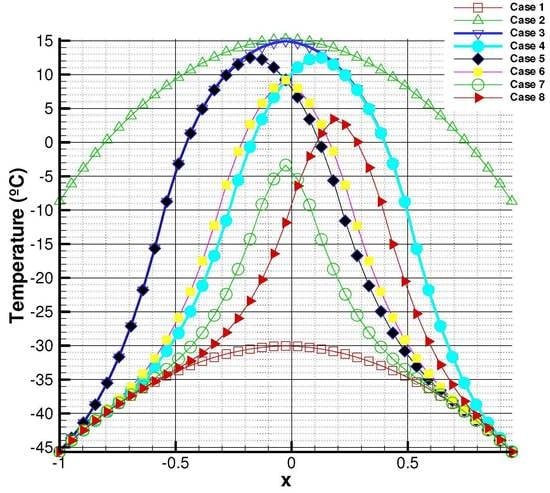
In Figure 2, Figure 3 and Figure 4, several stationary solutions for three different values of the solar constant, namely $Q=100,250,400$, are displayed. We note that both $Q=100$ and $Q=400$ belong to regions where the stationary solution is unique. When the value of the solar constant is $Q=250$, a multiplicity of stationary solutions appears. It can be noted that eight different solutions have been obtained, although more could be achieved while using other initial states.

In addition, it can be checked, in Figure 2, that the temperature is below zero for all of the latitudes (since the x coordinate represents the sine of the latitude). The reason behind is that, for those small values of the solar constant, the Earth receives little radiation and, as a consequence, a complete glaciation process takes place. This could have happened during the glacial periods of the Earth, which took place between 110,000 and about 15,000 years ago.

On the other hand, as displayed in Figure 4, when the solar constant take values $Q>Q_4=425$, the unique stationary solution is positive for all latitudes and, hence, there is absence of ice throughout the Earth’s surface. This is due to the high values of the incoming solar radiation.

As expressed before, the current value of the solar constant is $Q\approx 340$, which corresponds to a multiplicity of equilibrium states.

In Figure 5, it is displayed, in a $x-t$ plot, the evolution of the solutions of the EBM model towards the stationary solution for a value of the solar constant $Q=197$. It can be verified that, for this particular value of the solar constant, the stationary solution is negative for all latitudes.

In Figure 6, it is shown the evolution towards the stationary solution taking $Q=300$, which corresponds to the region of multiple stationary solutions, taking two constant different initial conditions $u(x,0)<-10$ °C and $u(x,0)>-10$ °C. We observe that, when the initial condition is a constant below $-10$ °C, the stationary temperatures attained are negative for all latitudes, while when taking an initial condition constant over $-10$ °C, the equilibrium state achieved takes values (that is, temperatures), ranging from positive to negative, depending on the latitude.

5.2. Coupled Model

The stationary solutions of the coupled model, as given in (8), are achieved by the same procedure as in the non-coupled case that is, evolving in time the evolution problem until the steady state solution is achieved, taking 1000 values of the solar constant and using the same initial conditions (Cases 1 to 8), as before. Figure 7 shows the approximation to the bifurcation diagram accomplished in this case.

We zoom in the previous figure and achieve the plot shown in Figure 8 in order to clearly identify the regions with unique or multiple solutions.

Similar regions, as in the non-coupled situation, of unique and multiple stationary solutions show up. In order to visualize some of these solutions, the results for the values of the solar constant $Q=100,250,400$ are depicted in Figure 9, Figure 10 and Figure 11.

In Figure 12, a comparison of the diagrams that were obtained for both the coupled and non-coupled model is displayed. We observe that the thermal oscillation between highest and lowest values of the temperature is larger in the coupled model than in the non-coupled one, which agrees with the thermostatic effect of the ocean.

The thermostatic effect is also patent in the results shown in Figure 13, where several stationary solutions for $Q=250$ are displayed.

6. Conclusions and Discussion

In this work, we have obtained, by numerical simulation, the equilibrium states and a subset of a $\left\{\right(Q,u\left)\right\}$ bifurcation diagram, where Q is the solar constant and u is the surface temperature. The climate model considered is composed of an Energy Balance Model and a deep ocean model. In order to obtain the stationary solutions, we have evolved in time the numerical solution computed by means of a finite volume method with a third order TVD Runge-Kutta approach for time integration, and a WENO method for spatial reconstruction.

We have achieved the stationary states of the EBM, without influence of the deep ocean, and also of the coupling EBM-deep ocean. The reason to consider these situations is that they are both relevant in climatic modelling. In the case of EBMs, without an ocean effect, they are frequently used in many studies of global climate, as they allow to predict the average surface temperature of the Earth due to incoming solar radiation, emission of radiation, energy absorption or greenhouse effects. The inclusion of the ocean effect has an important influence on the temperatures distribution due to the well-known thermostatic effect of the ocean, absorbing solar radiation and releasing it. Hence, we have dealt first with the non-coupled model, which is, solving just the Energy Balance Model without influence of the deep-ocean and then with the coupled model (surface-deep ocean), obtaining the approximation of the subset of the $\left\{\right(Q,u\left)\right\}$ diagram, which has been achieved solving the problem taking 1000 values of the solar constant Q and using several different initial conditions for every value of Q. Three different regions have been obtained in the diagram, two of them where there is a unique equilibrium solution for each value of Q and the other one where there exists a multiplicity of equilibrium states for each particular value of Q. This result agrees with a theorem put forward by Diaz, Tello [39], where the authors prove that, in the multiplicity of equilibrium states region, there are at least three stationary solutions (that is, more than three). In the present work, we have obtained eight of those solutions, which are non-constant and stable. The results of both situations (EBM without and with the effect of the deep ocean) have been similar, although with different stationary solutions in the plot $\left\{\right(Q,u\left)\right\}$. Actually, a comparison have been performed between both situations, observing that, when the ocean effect is considered, the thermal oscillation, which is difference between higher and lower temperatures, is lower than when its effect is not taken into account. This agrees with the well-known thermostatic effect of the ocean. It has also been pointed out that the current situation in the Earth corresponds to the value $Q\approx 340$, which is within the multiplicity region which gives rise to temperatures that oscillate from negative to positive values in the different latitudes. Additionally, it has been indicated in this work that the region with a unique negative stationary solution for each value of Q may correspond to glaciation periods.

References

- Budyko, M.I. The effect of solar radiation variations on the climate of the Earth. Tellus 1969, 21, 611–619. [Google Scholar] [CrossRef] [Green Version]
- Sellers, W.D. A Global Climatic Model Based on the Energy Balance of the Earth-Atmosphere System. J. Appl. Meteorol. 1969, 8, 392–400. [Google Scholar] [CrossRef]
- Díaz, J.I. On the mathematical treatment of energy balance climate models. In The Mathematics of Models for Climatology and Environment; Díaz, J.I., Ed.; Springer: Berlin/Heidelberg, Germany, 1997; pp. 217–251. [Google Scholar]
- North, G.R. Multiple solutions in energy balance climate models. Palaeogeogr. Palaeoclimatol. Palaeoecol. 1990, 82, 225–235. [Google Scholar] [CrossRef]
- Hetzer, G. The structure of the principal component for semilinear diffusion equations from energy balance climate models. Houst. J. Math. 1990, 16, 203–216. [Google Scholar]
- Díaz, J.; Hetzer, G.; Tello, L. An energy balance climate model with hysteresis. Nonlinear Anal. Theory Methods Appl. 2006, 64, 2053–2074. [Google Scholar] [CrossRef]
- Ghil, M.; Childress, S. Topics in geophysical fluid dynamics atmospheric dynamics, dynamo theory, and climate dynamics. In Applied Mathematical Sciences; Springer: New York, NY, USA, 1987. [Google Scholar] [CrossRef]
- Watts, R.G.; Morantine, M. Rapid climatic change and the deep ocean. Clim. Chang. 1990, 16, 83–97. [Google Scholar] [CrossRef]
- Díaz, J.I.; Tello, L. A nonlinear parabolic problem on a Riemannian manifold without boundary arising in climatology. Collect. Math. 1999, 50, 19–51. [Google Scholar]
- Diaz, J.I.; Tello, L. A 2D climate energy balance model coupled with a 3D deep ocean model. Electron. J. Differ. Equ. 2007, 16, 129–135. [Google Scholar]
- Bermejo, R.; Carpio, J.; Diaz, J.; Tello, L. Mathematical and numerical analysis of a nonlinear diffusive climate energy balance model. Math. Comput. Model. 2009, 49, 1180–1210. [Google Scholar] [CrossRef]
- Bermejo, R.; Carpio, J.; Díaz, J.I.; Galán del Sastre, P. A Finite Element Algorithm of a Nonlinear Diffusive Climate Energy Balance Model. Pure Appl. Geophys. 2008, 165, 1025–1047. [Google Scholar] [CrossRef]
- Díaz, J.I.; Hidalgo, A.; Tello, L. Multiple solutions and numerical analysis to the dynamic and stationary models coupling a delayed energy balance model involving latent heat and discontinuous albedo with a deep ocean. Proc. R. Soc. A 2014. [Google Scholar] [CrossRef] [Green Version]
- Hidalgo, A.; Tello, L. A Finite Volume Scheme for Simulating the Coupling between Deep Ocean and an Atmospheric Energy Balance Model. In Modern Mathematical Tools and Techniques in Capturing Complexity; Springer: Berlin/Heidelberg, Germany, 2011; pp. 239–255. [Google Scholar] [CrossRef]
- LeVeque, R.J. Finite-Volume Methods for Hyperbolic Problems; Cambridge University Press: Cambridge, UK, 2002. [Google Scholar]
- Godunov, S. A Difference Scheme for Numerical Solution of Discontinuous Solution of Hydrodynamic Equations. Math. Sb. 1959, 47, 271–306. [Google Scholar]
- Toro, E. Riemann Solvers and Numerical Methods for Fluid Dynamics: A Practical Introduction; Springer: Berlin/Heidelberg, Germany, 2009. [Google Scholar]
- Vázquez-Cendón, M. Solving Hyperbolic Equations with Finite Volume Methods; Springer International Publishing: Cham, Switzerland, 2015. [Google Scholar]
- Harten, A.; Engquist, B.; Osher, S.; Chakravarthy, S.R. Uniformly High Order Accurate Essentially Non-oscillatory Schemes, III. J. Comput. Phys. 1997, 131, 3–47. [Google Scholar] [CrossRef]
- Liu, X.D.; Osher, S.; Chan, T. Weighted Essentially Non-oscillatory Schemes. J. Comput. Phys. 1994, 115, 200–212. [Google Scholar] [CrossRef] [Green Version]
- Shu, C. Essentially Non-Oscillatory and Weighted Essentially Non-Oscillatory Schemes for Hyperbolic Conservation Laws. In Advanced Numerical Approximation of Nonlinear Hyperbolic Equations; Springer: Berlin/Heidelberg, Germany, 2006. [Google Scholar]
- Balsara, D.S.; Shu, C.W. Monotonicity Preserving Weighted Essentially Non-oscillatory Schemes with Increasingly High Order of Accuracy. J. Comput. Phys. 2000, 160, 405–452. [Google Scholar] [CrossRef] [Green Version]
- Titarev, V.; Toro, E. Finite-volume WENO schemes for three-dimensional conservation laws. J. Comput. Phys. 2004, 201, 238–260. [Google Scholar] [CrossRef]
- Dumbser, M.; Zanotti, O.; Hidalgo, A.; Balsara, D.S. ADER-WENO finite volume schemes with space–time adaptive mesh refinement. J. Comput. Phys. 2013, 248, 257–286. [Google Scholar] [CrossRef] [Green Version]
- Dumbser, M.; Hidalgo, A.; Zanotti, O. High order space-time adaptive ADER-WENO finite volume schemes for non-conservative hyperbolic systems. Comput. Methods Appl. Mech. Eng. 2014, 268, 359–387. [Google Scholar] [CrossRef] [Green Version]
- Levy, D.; Puppo, G.; Russo, G. Central WENO schemes for hyperbolic systems of conservation laws. ESAIM Modél. Math. Anal. Numér. 1999, 33, 547–571. [Google Scholar] [CrossRef]
- Levy, D.; Nayak, S.; Shu, C.; Zhang, Y. Central WENO schemes for Hamilton-Jacobi equations on triangular meshes. SIAM J. Sci. Comput. 2006, 28, 2229–2247. [Google Scholar] [CrossRef] [Green Version]
- Dumbser, M.; Boscheri, W.; Semplice, M.; Russo, G. Central Weighted ENO Schemes for Hyperbolic Conservation Laws on Fixed and Moving Unstructured Meshes. SIAM J. Sci. Comput. 2017, 39, A2564–A2591. [Google Scholar] [CrossRef]
- Castro, M.J.; Semplice, M. Third- and fourth-order well-balanced schemes for the shallow water equations based on the CWENO reconstruction. Math. Comput. Model. 2019, 89, 304–325. [Google Scholar] [CrossRef]
- Baeza, A.; Bürger, R.; Mulet, P.; Zorío, D. Central WENO Schemes Through a Global Average Weight. J. Sci. Comput. 2019, 78, 499–530. [Google Scholar] [CrossRef]
- Baeza, A.; Bürger, R.; Mulet, P.; Zorío, D. On the Efficient Computation of Smoothness Indicators for a Class of WENO Reconstructions. J. Sci. Comput. 2019, 80, 1240–1530. [Google Scholar] [CrossRef]
- Baeza, A.; Bürger, R.; Mulet, P.; Zorío, D. An Efficient Third-Order WENO Scheme with Unconditionally Optimal Accuracy. SIAM J. Sci. Comput. 2020, 42, A1028–A1051. [Google Scholar] [CrossRef]
- Balsara, D.S.; Garain, S.; Florinski, V.; Boscheri, W. An efficient class of WENO schemes with adaptive order for unstructured meshes. J. Comput. Phys. 2020, 404, 109062. [Google Scholar] [CrossRef]
- Shu, C.W.; Osher, S. Efficient implementation of essentially non-oscillatory shock-capturing schemes. J. Comput. Phys. 1988, 77, 439–471. [Google Scholar] [CrossRef] [Green Version]
- Gottlieb, S.; Shu, C.W. Total Variation Diminishing Runge-Kutta schemes. Math. Comput. 1998, 67, 73–85. [Google Scholar] [CrossRef] [Green Version]
- Harten, A. High resolution schemes for hyperbolic conservation laws. J. Comput. Phys. 1983, 49, 357–393. [Google Scholar] [CrossRef] [Green Version]
- Cannarsa, P.; Malfitana, M.; Martínez, P. Parameter Determination for Energy Balance Models with Memory. In Mathematical Approach to Climate Change and Its Impacts; Cannarsa, P., Mansutti, D., Provenzale, A., Eds.; Springer INdAM Series; Springer: Berlin/Heidelberg, Germany, 2020. [Google Scholar] [CrossRef] [Green Version]
- Floridia, G. Approximate controllability for nonlinear degenerate parabolic problems with bilinear control. J. Differ. Equ. 2014, 257, 3382–3422. [Google Scholar] [CrossRef]
- Díaz, J.I.; Tello, L. On a climate model with a dynamic nonlinear diffusive boundary condition. Discret. Contin. Dyn. Syst. S 2008, 1, 253. [Google Scholar] [CrossRef]
- Díaz, J.I.; Hernández, J.; Tello, L. On the Multiplicity of Equilibrium Solutions to a Nonlinear Diffusion Equation on a Manifold Arising in Climatology. J. Math. Anal. Appl. 1997, 216, 593–613. [Google Scholar] [CrossRef] [Green Version]
- Hetzer, G. The shift-semiflow of a multi-valued evolution equation from climate modelling. Nonlinear Anal. Theory Methods Appl. 2001, 47, 2905–2916. [Google Scholar] [CrossRef]
- Hetzer, G. The number of stationary solutions for a one-dimensional Budyko-type climate model. Nonlinear Anal. Real World Appl. 2001, 2, 259–272. [Google Scholar] [CrossRef]
- Díaz, J.I.; Tello, L. Infinitely many stationary solutions for a simple climate model via a shooting method. Math. Methods Appl. Sci. 2002, 25, 327–334. [Google Scholar] [CrossRef]
- Arcoya, D.; Diaz, J.; Tello, L. S-Shaped Bifurcation Branch in a Quasilinear Multivalued Model Arising in Climatology. J. Differ. Equ. 1998, 150, 215–225. [Google Scholar] [CrossRef] [Green Version]
- Stone, P.H. A simplified radiative-dynamical model for the static stability of rotating atmospheres. J. Atmos. Sci. 1972, 29, 405–418. [Google Scholar] [CrossRef] [Green Version]
- Díaz, J.I. Mathematical analysis of some diffusive energy balance models in Climatology. In Mathematics, Climate and Environment; Díaz, J.I., Lions, J.L., Eds.; Research Notes in Applied Mathematics n° 27; Masson: Paris, France, 1993; pp. 28–56. [Google Scholar]
- Hidalgo, A.; Tello, L. On a climatological energy balance model with continents distribution. Discret. Continu. Dyn. Syst. A 2015, 35, 1503. [Google Scholar] [CrossRef]
- Jiang, G.S.; Shu, C.W. Efficient Implementation of Weighted ENO Schemes. J. Comput. Phys. 1996, 126, 202–228. [Google Scholar] [CrossRef] [Green Version]
- Cravero, I.; Puppo, G.; Semplice, M.; Visconti, G. CWENO: Uniformly accurate reconstructions for balance laws. Math. Comp. 2018, 87, 1689–1719. [Google Scholar] [CrossRef] [Green Version]
- Toro, E.F.; Millington, R.C.; Nejad, L.A.M. Towards Very High Order Godunov Schemes. In Godunov Methods; Toro, E.F., Ed.; Springer: Boston, MA, USA, 2001; pp. 907–940. [Google Scholar]
- Titarev, V.; Toro, E. ADER: Arbitrary High Order Godunov Approach. J. Sci. Comput. 2002, 17, 609–618. [Google Scholar] [CrossRef]
- Toro, E.F.; Hidalgo, A. ADER finite volume schemes for nonlinear reaction diffusion equations. Appl. Numer. Math. 2009, 59, 73–100. [Google Scholar] [CrossRef]
- Gassner, G.; Loercher, F.; Munz, C.D. A contribution to the construction of diffusion fluxes for finite volume and Discontinuous Galerkin schemes. J. Comput. Phys. 2007, 224, 1049–1063. [Google Scholar] [CrossRef]
- Hidalgo, A.; Tello, L.; Toro, E.F. Numerical and analytical study of an atherosclerosis inflammatory disease model. J. Math. Biol. 2014, 68, 1785–1814. [Google Scholar] [CrossRef] [Green Version]
Figure 1.
Approximated diagram for the non-coupled model. is the constant stationary solution for the value .
Figure 2.
Stationary solution of the Energy Balance Model (EBM) model, without coupling with the deep ocean, for .
Figure 3.
Several stationary solutions of the EBM model, without coupling with the deep ocean, for . This is the region of multiple stationary solutions.
Figure 4.
Stationary solution of the EBM model, without coupling with the deep ocean, for .
Figure 5.
Evolution towards the stationary solution taking as solar constant . The stationary temperatures are negative for all latitudes.
Figure 6.
Evolution towards the stationary solution taking as solar constant taking an initial condition °C (a) and °C (b).
Figure 7.
Approximated diagram for the coupled model.
Figure 8.
Detail of the Approximated diagram for the coupled model.
Figure 9.
Unique stationary solution. Coupled model. .
Figure 10.
Multiple stationary solutions. Coupled model. .
Figure 11.
Figure 12.
Approximated diagrams for the coupled and the non-coupled model.
Figure 13.
Several stationary solutions for obtained for the EBM (a) and Coupled model (b).