
Qualitative Analyses of Differential Systems with Time-Varying Delays via Lyapunov–Krasovskiĭ Approach


1
Department of Mathematics, Faculty of Sciences, Van Yuzuncu Yil University, Campus, Van 65080, Turkey
2
Department of Computer Programing, Baskale Vocational School, Van Yuzuncu Yil University, Campus, Van 65080, Turkey
3
Department of Mathematics, Zhejiang Normal University, Jinhua 321004, China
4
Research Center for Interneural Computing, China Medical University Hospital, China Medical University, Taichung 404332, Taiwan
*
Author to whom correspondence should be addressed.
†
These authors contributed equally to this work.
Mathematics 2021, 9(11), 1196; https://doi.org/10.3390/math9111196
Submission received: 16 April 2021
/
Revised: 20 May 2021
/
Accepted: 21 May 2021
/
Published: 25 May 2021
(This article belongs to the Special Issue Mathematical Analysis and Analytic Number Theory 2020)
Abstract
:In this paper, a class of systems of linear and non-linear delay differential equations (DDEs) of first order with time-varying delay is considered. We obtain new sufficient conditions for uniform asymptotic stability of zero solution, integrability of solutions of an unperturbed system and boundedness of solutions of a perturbed system. We construct two appropriate Lyapunov–Krasovskiĭ functionals (LKFs) as the main tools in proofs. The technique of the proofs depends upon the Lyapunov–Krasovskiĭ method. For illustration, two examples are provided in particular cases. An advantage of the new LKFs used here is that they allow to eliminate using Gronwall’s inequality. When we compare our results with recent results in the literature, the established conditions are more general, less restrictive and optimal for applications.
Keywords:
system of non-linear DDEs; uniformly asymptotically stability; integrability; boundedness at infinity; Lyapunov–Krasovskiĭ approach; time-varying delayMSC:
34D05; 34K20; 45J051. Introduction
From the relevant literature, it can be observed that numerous processes, both natural and human-made, in biology, interaction of species, population dynamics, microbiology, distributed networks, learning models, mechanics, medicine, nuclear reactors, chemistry, distributed networks, epidemiology, physics, engineering, economics, physiology, viscoelasticity, as well as many others, involve time delays. Hence, many applications in sciences, engineering and so on can be modeled as differential equations with time-varying delays (see the books of Burton [1], Hale and Verduyn Lunel [2], Kolmanovski and Nosov [3], Krasovskiĭ [4], Kuang [5], Lakshmikantham et al. [6], Smith [7] and bibliographies therein).
The interest of applied mathematicians, engineers, etc., to investigate qualitative properties of solutions for such numerous problems with time-varying delays has increased considerably in the last decades. In particular, see the mentioned books, the papers of Arino et al. [8], Azbelev et al. [9], Berezansky and Braverman [10], Du [11], Gil [12], Graef and Tunç [13], Slyn’ko and Tunç [14], Tian and Ren [15], Tunç [16,17,18], Tunç and Erdur [19], Tunç and Golmankhaneh [20], Tunç and Tunç [21,22,23], Zevin [24] and bibliographies therein.
It is worth mentioning that especially DDEs of first and second order with constant and time-varying delays can be encountered intensively during investigations and applications. For those reasons, during the investigations and applications, it is required to get information about various qualitative behaviors of solutions of those kind of equations such as stability, instability, convergence, etc., of solutions of DDEs. To the best of available information, it should be noted that from the theory of DDEs, we know that analytically solving DDEs with time-varying delays is a very difficult mathematical task. Therefore, over the past decades, some methods have been developed to get information about the qualitative properties of solutions of DDEs without solving them. Among the developed methods, the Lyapunov’s second method, Lyapunov–Krasovskiĭ method, Razumikhin method and fixed point method can be effectively used to investigate the stability and some other properties of solutions of ODEs, DDEs, neutral and advanced functional differential equations. In general, the Lyapunov’s second method is used to discuss numerous qualitative properties of ODEs of first and higher order. Next, the Razumikhin method is only used to study qualitative properties of a few certain forms of DDEs and impulsive differential equations. As for the fixed point method, it can be used to study stability, existence of periodic solutions, etc., of various kind of those equations of first order. However, this method is rarely used in the equations of second order and those of higher order. Meanwhile, during the last 50 years, the theory of functional differential equations (FDEs) has been developed extensively. Krasovskiĭ [4] firstly investigated the stability of equilibria and wanted to make sure that all of the results for ODE using LKFs could be carried over to DDEs. It should be noted Krasovskiĭ [4] suggested the use of functional defined on DDEs’ trajectories instead of Lyapunov functions. Later, this functional method is very effectively used to get information on the mentioned properties of solutions of DDEs without having any prior information of solutions. When Lyapunov–Krasovskiĭ method is used during the investigations, it is needed to define or construct a suitable LKF, which is positive definite, and its time derivative along the considered DDEs is negative or negative-semi definite. From this point of view, finding a suitable Lyapunov–Krasovskiĭ functional for a problem under study is difficult and an open problem in the literature by this time. Next, most of researches on DDEs focus on linear differential equations with constant delay and preservation of stability; however, the number of available researches on scalar nonlinear DDEs and nonlinear system of DDEs with time-varying delays are less. From this point, it deserves to investigate the properties of solutions of systems of nonlinear DDEs with time-varying delays.
The motivation of this paper was inspired by a recent work of Tian and Ren [15]. From this point of view, we mention a related work of Tian and Ren [15]. In 2020, Tian and Ren [15] considered the following system of linear DDEs with time-varying delay,
where , and is the time-varying delay, and it satisfies
Tian and Ren [15] defined an LKF for the system of DDEs (1). Based on that LKF, Tian and Ren [15] proved a theorem, ([15], Theorem 1), on the asymptotically stability of the system of DDEs (1).
In this paper, motivated by the system of DDEs (1), the result of Tian and Ren ([15], Theorem 1) and those in the bibliography of this paper, as an alternative to the linear system of DDEs (1), we consider a nonlinear system of DDEs with time-varying delay as follows:
with the continuous initial function
where , , is the time-varying delay, which satisfies the condition (2), , , , and .
We now summarize the aim of this paper by the following items, respectively:
- (1)
- We investigate the uniformly asymptotically stability of zero solution of the system of DDEs (1), see Theorem 3. To investigate this problem, we define a very different LKF from that in Tian and Ren [15].
- (2)
- We study the uniformly asymptotically stability of zero solution and the integrability of the norm of solutions of the following unperturbed nonlinear system of DDEs by Theorem 4 and Theorem 5, respectively:
- (3)
- We investigate the boundedness of solutions of the perturbed system of nonlinear DDEs (3), see Theorem 6.
- (4)
- In particular cases, two new examples and graphs of their solutions are provided to show applications of Theorems 3–6.
2. Basic Result
Consider the system of the DDEs:
where , and takes bounded sets into bounded sets. For some , denotes the space of continuous functions . For any , and , we have for and .
Let . The norm is defined by . Next, let . For this case, the matrix norm, is defined by .
In this article, without loss of generality, sometimes instead of , we will simply write x.
For any , let
and
We suppose that the function H satisfies the conditions of the uniqueness of solutions of the system of DDEs (5). We note that the system of DDEs (3) is a particular case of the system of DDEs (5).
Let be a solution of the system of DDEs (5) such that on , where is an initial function.
Let
be a continuous functional in t and with . Further, let denote the derivative of on the right through any solution of the system of DDEs (5).
Theorem 1
(Burton [1], Theorem 4.2.9). Assume that the following conditions hold:
- (A1)
- The function satisfies the locally Lipschitz in x, i.e., for every compact and , there exists a with such thatfor all and .
- (A2)
- Let be a functional such that it satisfies the one side locally Lipschitz in t:whenever , where is continuous.
- (A3)
- There are four strictly increasing functions ω, , , with value 0 at 0 such thatandwhenever and . Then, the solution of the system of DDEs (5) is uniformly asymptotically stable.
3. Asymptotic Stability
Firstly, we introduce the main result of Tian and Ren ([15], Theorem 1).
Theorem 2
(Tian and Ren [15], Theorem 1). For given scalars , system (1) is asymptotically stable if there exist matrices , such that
holds for where
and
is defined as
We now give our first result.
Theorem 3.
We suppose that the following conditions (C1) and (C2) hold:
- (C1)
- There exist constants from (2) and such that
- (C2)
- There exist a constant from (C1) such that
Then, the zero solution of the system of DDEs (1) is uniformly asymptotically stable
Proof.
Define a new LKF by
where is an arbitrary positive constant which will be chosen later in the proof.
This functional, the LKF (6), can be expressed as the following:
Then, we see that the functional satisfies the following relations:
Thus, it is obvious that the LKF is positive definite.
Let
In the light of Burton ([1], Theorem 4.2.9), we define the functional as follows:
From this point of view, we have
Next, it follows that
where
Hence, we arrive at the inequality:
This inequality proves that the functional satisfies the locally Lipschitz condition in x, i.e., the condition (A1) of Theorem 1 holds.
For the next step, in view of the definition of , it follows that
Thus,
For the next step, via some simple calculations, we get
where
This result proves that the condition (A2) of Theorem 1 holds.
The derivative of in (6) with respect to the system of DDEs (1) is given by
Using the condition (C2), we obtain
Thereby, gathering the relations (7) and (8) and using the condition , we find
Let .
Then, we have
Using the condition (C1), we have
where, . □
Thus, we discover that the time derivative of the LKF is negative definite. This is a desirable and necessary result for the investigation of uniform asymptotic stability.
From the inequality (9), it follows that the condition (A3) of Theorem 1 is satisfied. From the whole discussion, we see that the conditions of (A1)–(A3) of Theorem 1 hold (see Burton ([1], Theorem 4.2.9). Therefore, the zero solution of the nonlinear system of DDEs (4) is uniformly asymptotically stable.
4. Uniformly Asymptotic Stability and Integrability
In the nonlinear system of DDEs (3), we take Then, we consider the unperturbed nonlinear system of DDEs (4). We now generalize and optimize the main result of Tian and Ren ([15], Theorem 1) under less restrictive conditions and also give one more result for the non-linear system of DDEs (4). These results are proved by the Lyapunov–Krasovskiĭ functional approach.
Theorem 4.
We suppose that the following conditions (H1) and (H2) hold:
- (H1)
- There exist a constant such that
- (H2)
- There exist constants and from (2) and (H1), respectively, and , such thatand
Then, the zero solution of the system of DDEs (4) is uniformly asymptotically stable.
Proof.
Define a new LKF by
where is an arbitrary positive constant, which will be chosen in the proof.
This functional can be expressed as the following:
Then, we see that the functional satisfies the following relations:
Let
and define
Hence, it follows that
Next, using the condition (H2) and following some simple calculations, we get
where
Hence, we conclude the inequality
This inequality proves that the functional satisfies the local Lipschitz condition in x. Thus, the condition (A1) of Theorem 1 holds.
For the next step, from the definition of and the condition (H2), it follows that
Thus, it follows that
As the following step, using some simple calculations and the condition (H2), we have
where
The last inequality shows that the condition (A2) of Theorem 1 holds.
The derivative of in (10) along the system of DDEs (4) is given by
Consider the first term on the right hand side of the equality (11). Using the condition (H1), we obtain
Thereby, gathering the inequalities (11), (12) and using the condition , we have
Choosing as , we have
Using the condition (H2), we conclude that
where . □
As in the proof of Theorem 3, we find that the time derivative of the LKF is negative definite. From the inequality (13), it follows that the condition (A3) of Theorem 1 is satisfied. From the whole discussion of this proof, it can be followed that the conditions of (A1)–(A3) of Theorem 1 hold (see Burton ([1], Theorem 4.2.9)). Therefore, the zero solution of the nonlinear system of DDEs (4) is uniformly asymptotically stable.
Theorem 5.
If the conditions (H1) and (H2) of Theorem 4 hold, then the norm of solutions of the system of DDEs (4) is integrable in the sense of Lebesgue on .
Proof.
As in the proof of Theorem 4, the main tool in this proof is the LKF . It is clear that the conditions (H1) and (H2) yield that
This result verifies that the LKF is decreasing. That is, the LKF satisfies that
Then, integrating this inequality from to t, we obtain
for all .
Then, we find that
If , then the last inequality clearly implies that
Therefore, we can conclude that the norm of solutions of the system of DDEs (4) is integrable in the sense of Lebesgue on . Thus, the proof of Theorem 5 is completed. □
Example 1.
Consider the following two dimensional system of non-linear DDEs:
where is time-varying delay, .
Then, comparing both the systems of DDEs (14) and DDEs (4), it follows that
Let
and
In view of the matrix , we have
since
Hence, we derive
Next, some simple calculations give
and
It follows that the conditions (C1), (C2) of Theorem 3 and (H1) and (H2) of Theorems 4, 5 hold. So, the solution of the system of DDEs (14) is uniformly asymptotic stable. Furthermore, the norm of solutions of the system of DDEs (14) is integrable.
5. Boundedness
For the boundedness of the solutions of the system of nonlinear DDEs (3), we need the following condition in addition to some of those above, (H1):
- (H3)
- There exist positive constants , , from (H2) and a function such that
Theorem 6.
If the conditions (H1) and (H3) hold, then the solutions of the system of DDEs (3) are bounded as .
Proof.
As in the proofs of the former theorems, the main tool in this proof is the LKF . From the conditions (H2) and (H3), we can arrive at
Hence, using condition (H3), we derived that
Integrating this inequality, we obtain
Using (15) and the definition the definition of the LKF , we derive that
From the first and last terms of (16), we derive
By the calculating the limit as , it is derived from the last inequality that
Then, we conclude that the solutions of the system of nonlinear DDEs (3) are bounded as . The proof of Theorem 6 is now completed. □
Example 2.
Consider the following perturbed system of DDEs:
where is time-varying delay, .
When the non-linear systems of DDEs (17) and DDEs (3) are compared here, we do not need to show the satisfaction of the conditions related to the matrix , the function and the time-varying delay function , which have been shown in Example 1. In this case, we first consider the function
For the next step, for all , we have:
where
Next, we have
Thus, all the conditions of Theorem 6 hold. In view of the above discussion, we can conclude that all the solutions of the system of DDEs (17) are bounded as .
6. Discussion and Contribution
We now outline the contributions of Theorems 3–6 to the topic of the paper and the available related literature.
- (1)
- It follows that the systems of DDEs (3) and DDEs (4) extend and improve the system of DDEs (1) of Tian and Ren ([15], Theorem 1) from linear case to the non-linear case.
- (2)
- This LKF was used as a main tool to prove Theorem 2 in Section 3 by the authors.At the next step, Tian and Ren ([15], Theorem 1) calculated the derivative of this LKF along the system of DDEs (1) and obtained the following relations:where
Based upon the results of Lemmas 1–4 (see [15]), Tian and Ren (cite15, Theorem 1) proved a result on the asymptotic stability of the linear system of DDEs (1) utilizing the LKF (18) and its time derivative in (19). In fact, the LKF (18) and its time derivative (19) satisfy the conditions of Lyapunov-Krasovskiĭ’s asymptotic stability theorem (see [1,2]). From this result, i.e., Theorem 2 of Section 3, a new and interesting delay-dependent stability criterion is derived in terms of the LMIs.
In this paper, we define two more convenient LKFs, the first one is given by (6) such that
In view of the first LKF and its time derivative, applying the famous result of Burton, (ref. [1], Theorem 4.2.9), we improve the result of Tian and Ren ([15], Theorem 1) under weaker conditions. In spite of Tian and Ren ([15], Theorem 1) investigating the asymptotic stability of the linear system of DDEs (1), we discuss the uniformly asymptotically stability of (1), such that the uniformly asymptotic stability implies asymptotic stability, but its converse is not true.
Next, it is worth mentioning that the main result of Tian and Ren ([15], Theorem 1) is very interesting and has a good scientific novelty. However, the weaker conditions of Theorem 3 can be clearly observed and checked if we compare the conditions of Tian and Ren ([15], Theorem 1) with those of Theorem 3, such that taking into account Lemmas 1–4 of Tian and Ren [15], the LKF (18) and its time derivative (19) and our LKF and its time derivative, i.e., (5) and (6), respectively. Here, indeed, when we compare the conditions of Theorem 3 with those of Tian and Ren ([15], Theorem 1), we see that the conditions of Theorem 3 are very convenient and much optimal, easier to verify and apply as seen in Example 1.
As the next step, we define the following LKF:
Then, we extend and improve the main result of Tian and Ren ([15], Theorem 1) for the uniformly asymptotically stability of the zero solution, the integrability of the norm of the solutions of the system of DDE (4) as well as for the boundedness of solutions of the system of DDEs (3) using this LKF. For the sake of the brevity, we will not give more details about proper discussions of Theorems 4–6. These are the novelty, originality and contributions of this paper. Next, the mentioned observations are desirable facts for proper works to be done in the literature on the topic.
- (3)
- In this paper, we give two examples. These examples satisfy the conditions of Theorems 3–6 and verify the applications of the results of this paper.
- (4)
- An advantage of the new LKFs used here is that they eliminate using Gronwall’s inequality for the boundedness of solutions at infinity. Compared to related results in the literature, the conditions here are more general, simple, and convenient for application.
7. Conclusions
In this paper, a class of systems of DDEs with time-varying delay is considered. Four new results, which are given by Theorems 3–6, are proved on the uniformly asymptotically stability of zero solution and the integrability of solutions of two non-perturbed systems of DDEs as well as the boundedness of solutions of a perturbed system. The technique used in the proofs of Theorems 3–6 depends upon definitions of two new Lyapunov–Krasovskiĭ functionals. An advantage of the new LKFs used here is that they can lead to more optimal, general and less restrictive results for the given results, and also eliminate the need to use Gronwall’s inequality for the boundedness of solutions. Since Gronwall’s inequality is not used, the conditions for the boundedness of solutions are also more general, simple, and convenient to apply. Our results improve and extend the result of Tian and Ren ([15], Theorem 1), add three more new results on the qualitative properties of solutions. We give two examples to provide and to illustrate the applications of the new results of this paper.
Author Contributions
Conceptualization, C.T. and J.-C.Y.; Data curation, O.T.; Formal analysis, C.T., Y.W. and J.-C.Y.; Funding acquisition, Y.W.; Methodology, C.T., O.T. and Y.W.; Project administration, J.-C.Y.; Supervision, Y.W. and J.-C.Y.; Validation, C.T.; Visualization, O.T.; Writing—original draft, O.T. All authors have read and agreed to the published version of the manuscript.
Funding
This research received no external funding.
Conflicts of Interest
The authors declare no conflict of interest.
References
- Burton, T.A. Stability and Periodic Solutions of Ordinary and Functional Differential Equations; Corrected Version of the 1985 Original; Dover Publications, Inc.: Mineola, NY, USA, 2005. [Google Scholar]
- Hale, J.K.; Lunel, S.M.V. Introduction to Functional-Differential Equations; Applied Mathematical Sciences; Springer: New York, NY, USA, 1993; Volume 99. [Google Scholar]
- Kolmanovskii, V.B.; Nosov, V.R. Stability of Functional-Differential Equations; Mathematics in Science and Engineering; Academic Press, Inc. [Harcourt Brace Jovanovich, Publishers]: London, UK, 1986; Volume 180. [Google Scholar]
- Krasovskiĭ, N.N. Stability of motion. In Applications of Lyapunov’s Second Method to Differential Systems and Equations with Delay; Brenner, J.L., Translator; Stanford University Press: Stanford, CA, USA, 1963. [Google Scholar]
- Kuang, Y. Delay Differential Equations with Applications in Population Dynamics; Mathematics in Science and Engineering; Academic Press, Inc.: Boston, MA, USA, 1993; Volume 191. [Google Scholar]
- Lakshmikantham, V.; Wen, L.Z.; Zhang, B.G. Theory of Differential Equations with Unbounded Delay; Mathematics and Its Applications; Kluwer Academic Publishers Group: Dordrecht, The Netherlands, 1994; Volume 298. [Google Scholar]
- Smith, H. An Introduction to Delay Differential Equations with Applications to the Life Sciences; Texts in Applied Mathematics; Springer: New York, NY, USA, 2011; Volume 57. [Google Scholar]
- Arino, O.; Hbid, M.L.; Dads, E.A. Delay differential equations and applications. In Proceedings of the NATO Advanced Study Institute Held at the Cadi Ayyad University, Marrakech, Morocco, 9–21 September 2002; NATO Science Series II: Mathematics, Physics and Chemistry. Springer: Dordrecht, The Netherlands, 2006; Volume 205. [Google Scholar]
- Azbelev, N.; Maksimov, V.; Rakhmatullina, L. Introduction to the theory of linear functional-differential equations. In Advanced Series in Mathematical Science and Engineering; World Federation Publishers Company: Atlanta, GA, USA, 1995; Volume 3. [Google Scholar]
- Berezansky, L.; Braverman, E. On stability of some linear and nonlinear delay differential equations. J. Math. Anal. Appl. 2006, 314, 391–411. [Google Scholar] [CrossRef] [Green Version]
- Du, X. Some kinds of Liapunov functional in stability theory of RFDE. Acta Math. Appl. Sin. (Engl. Ser.) 1995, 11, 214–224. [Google Scholar] [CrossRef]
- Gil, M.I. Stability of delay differential equations with oscillating coefficients. Electron. J. Differ. Equ. 2010, 2010, 1–5. [Google Scholar]
- Graef, J.R.; Tunç, C. Continuability and boundedness of multi-delay functional integro-differential equations of the second order. Rev. R. Acad. Cienc. Exactas Fís. Nat. Ser. A Mat. RACSAM 2015, 109, 169–173. [Google Scholar] [CrossRef]
- Slyn’ko, V.I.; Tunç, C. Instability of set differential equations. J. Math. Anal. Appl. 2018, 467, 935–947. [Google Scholar] [CrossRef]
- Tian, J.; Ren, Z. Stability analysis of systems with time-varying delays via an improved integral inequality. IEEE Access 2020, 8, 90889–90894. [Google Scholar] [CrossRef]
- Tunç, C. A note on boundedness of solutions to a class of non-autonomous differential equations of second order. Appl. Anal. Discrete Math. 2010, 4, 361–372. [Google Scholar] [CrossRef] [Green Version]
- Tunç, C. Uniformly stability and boundedness of solutions of second order nonlinear delay differential equations. Appl. Comput. Math. 2011, 10, 449–462. [Google Scholar]
- Tunç, C. Stability to vector Liénard equation with constant deviating argument. Nonlinear Dynam. 2013, 73, 1245–1251. [Google Scholar] [CrossRef]
- Tunç, C.; Erdur, S. New qualitative results for solutions of functional differential equations of second order. Discrete Dyn. Nat. Soc. 2018, 2018, 3151742. [Google Scholar] [CrossRef] [Green Version]
- Tunç, C.; Golmankhaneh, A.K. On stability of a class of second alpha-order fractal differential equations. AIMS Math. 2020, 5, 2126–2142. [Google Scholar] [CrossRef]
- Tunç, C.; Tunç, O. A note on certain qualitative properties of a second order linear differential system. Appl. Math. Inf. Sci. 2015, 9, 953–956. [Google Scholar]
- Tunç, C.; Tunç, O. On the boundedness and integration of non-oscillatory solutions of certain linear differential equations of second order. J. Adv. Res. 2016, 7, 165–168. [Google Scholar] [CrossRef] [Green Version]
- Tunç, C.; Tunç, O. A note on the stability and boundedness of solutions to non-linear differential systems of second order. J. Assoc. Arab. Univ. Basic Appl. Sci. 2017, 24, 169–175. [Google Scholar] [CrossRef]
- Zevin, A.A. Maximum Lyapunov exponents and stability criteria of linear systems with variable delay. J. Appl. Math. Mech. 2015, 79, 1–8. [Google Scholar] [CrossRef]
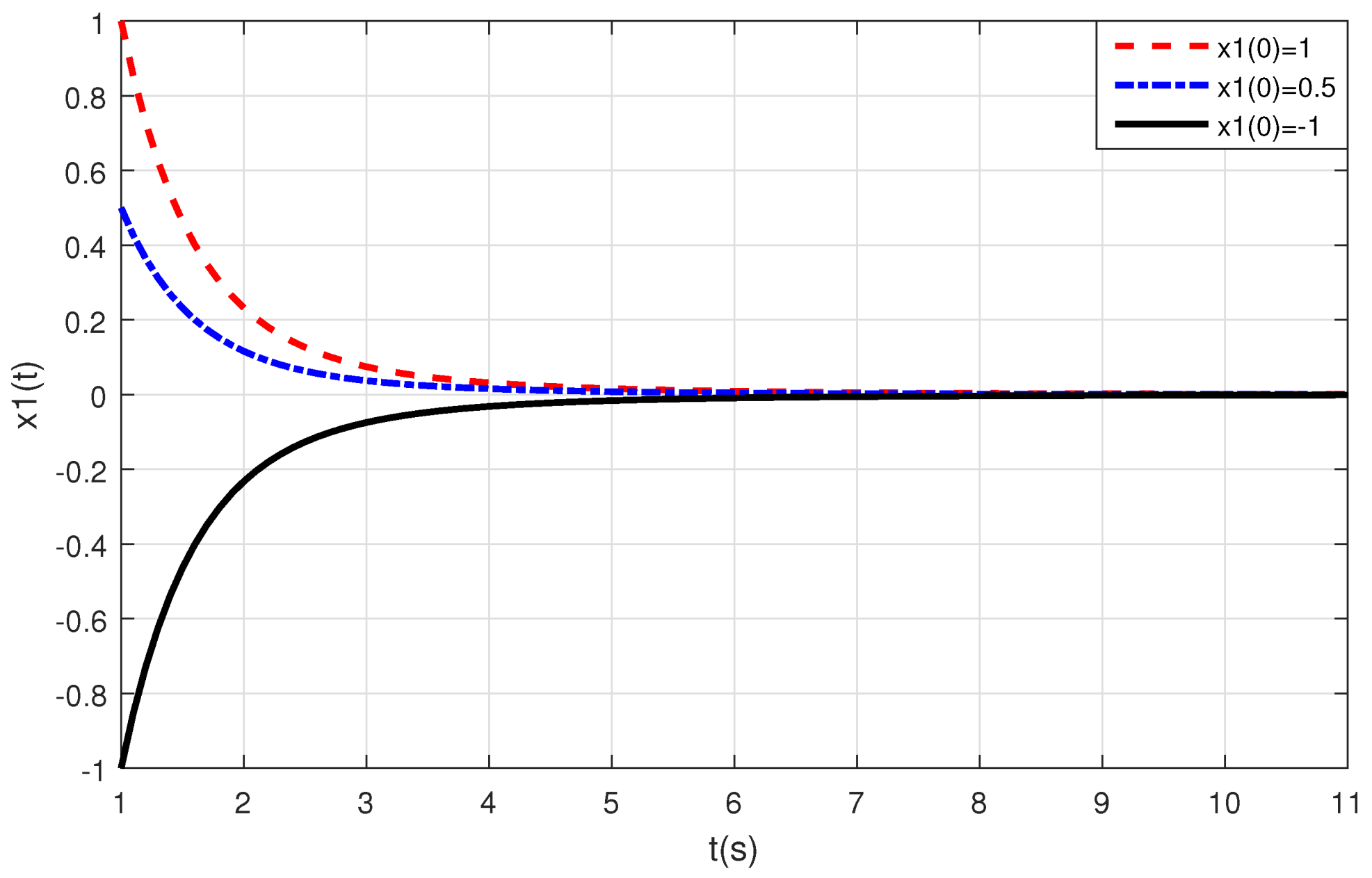
Figure 1.
This figure shows that the solution of the system of DDEs (14) is uniformly asymptotically stable and the norm of this solution is integrable for , and different initial values.
Figure 1.
This figure shows that the solution of the system of DDEs (14) is uniformly asymptotically stable and the norm of this solution is integrable for , and different initial values.

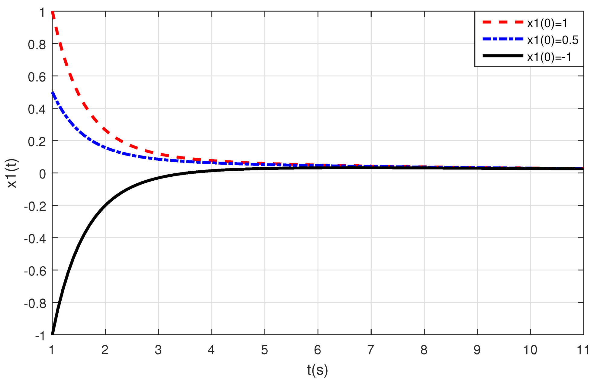
Figure 2.
This figure shows that the solution of the system of DDEs (14) is uniformly asymptotically stable and the norm of this solution is integrable for , and different initial values.
Figure 2.
This figure shows that the solution of the system of DDEs (14) is uniformly asymptotically stable and the norm of this solution is integrable for , and different initial values.

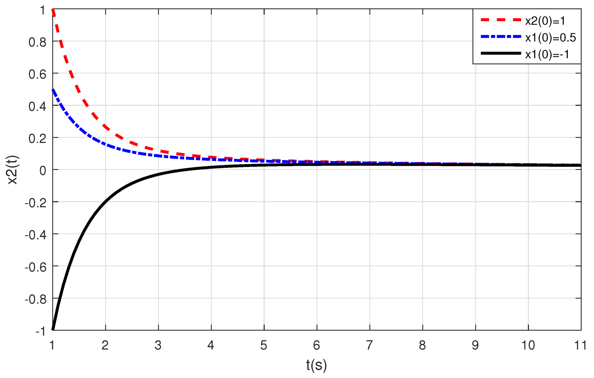
Figure 3.
This figure shows that the solution of the system of DDEs (17) is bounded for , and different initial values.
Figure 3.
This figure shows that the solution of the system of DDEs (17) is bounded for , and different initial values.

Figure 4.
This figure shows that the solution of the system of DDEs (17) is bounded for , and different initial values.
Figure 4.
This figure shows that the solution of the system of DDEs (17) is bounded for , and different initial values.

Publisher’s Note: MDPI stays neutral with regard to jurisdictional claims in published maps and institutional affiliations. |
© 2021 by the authors. Licensee MDPI, Basel, Switzerland. This article is an open access article distributed under the terms and conditions of the Creative Commons Attribution (CC BY) license (https://creativecommons.org/licenses/by/4.0/).
Share and Cite
MDPI and ACS Style
Tunç, C.; Tunç, O.; Wang, Y.; Yao, J.-C. Qualitative Analyses of Differential Systems with Time-Varying Delays via Lyapunov–Krasovskiĭ Approach. Mathematics 2021, 9, 1196. https://doi.org/10.3390/math9111196
AMA Style
Tunç C, Tunç O, Wang Y, Yao J-C. Qualitative Analyses of Differential Systems with Time-Varying Delays via Lyapunov–Krasovskiĭ Approach. Mathematics. 2021; 9(11):1196. https://doi.org/10.3390/math9111196
Chicago/Turabian StyleTunç, Cemil, Osman Tunç, Yuanheng Wang, and Jen-Chih Yao. 2021. "Qualitative Analyses of Differential Systems with Time-Varying Delays via Lyapunov–Krasovskiĭ Approach" Mathematics 9, no. 11: 1196. https://doi.org/10.3390/math9111196
Note that from the first issue of 2016, this journal uses article numbers instead of page numbers. See further details here.