
Impact of Material Stiffness and Anisotropy on Coaptation Characteristics for Aortic Valve Cusps Reconstructed from Pericardium


1
Marchuk Institute of Numerical Mathematics of the Russian Academy of Sciences, 119333 Moscow, Russia
2
Department of Hospital Surgery of N.V. Sklifosovsky, Institute of Clinical Medicine, Sechenov University, 8-2 Trubetskaya St., 119991 Moscow, Russia
3
Department of Cardiac Surgery, Central Clinical Hospital with Polyclinic of the Administrative Directorate of the President of the Russian Federation, 15 Marshal Timoshenko St., 121359 Moscow, Russia
4
Institute for Computer Science and Mathematical Modeling, Sechenov University, 8-2 Trubetskaya St., 119991 Moscow, Russia
*
Author to whom correspondence should be addressed.
Mathematics 2021, 9(18), 2193; https://doi.org/10.3390/math9182193
Submission received: 31 July 2021
/
Revised: 30 August 2021
/
Accepted: 3 September 2021
/
Published: 8 September 2021
(This article belongs to the Special Issue Mathematical Modelling in Biomedicine II)
Abstract
:The numerical assessment of reconstructed aortic valves competence and leaflet design optimization rely on both coaptation characteristics and the diastolic valve configuration. These characteristics can be evaluated by the shell or membrane formulations. The membrane formulation is preferable for surgical aortic valve neocuspidization planning since it is easy to solve. The results on coaptation zone sensitivity to the anisotropy of aortic leaflet material are contradictive, and there are no comparisons of coaptation characteristics based on shell and membrane models for anisotropic materials. In our study, we explore for the first time how the reduced model and anisotropy of the leaflet material affect the coaptation zone and the diastolic configuration of the aortic valve. To this end, we propose the method to mimic the real, sutured neo-leaflet, and apply our numerical shell and membrane formulations to model the aortic valve under the quasi-static diastolic pressure varying material stiffness and anisotropy directions. The shell formulation usually provides a lesser coaptation zone than the membrane formulation, especially in the central zone. The material stiffness does influence the coaptation zone: it is smaller for stiffer material. Anisotropy of the leaflet material does not affect significantly the coaptation characteristics, but can impact the deformed leaflet configuration and produce a smaller displacement.
1. Introduction
Aortic valve disease is among the most common cardiovascular conditions that affect elderly people. According to the recent studies [1], about 4.9 million and 2.7 million elderly patients are diagnosed with aortic stenosis in Europe and North America, respectively. Y. Do et al. demonstrated that the 5 year overall survival of untreated patients with moderate aortic stenosis is only 52.3% [2]. About 28% of patients with severe aortic stenosis undergo aortic valve replacement. This corresponds to 12,129 procedures in the U.S. between 2008 and 2016 [3]. However, the estimated need for aortic valve surgery is suggested to exceed 200,000 in North America and 300,000 in Europe. In 2018, the number of procedures was increased up to 73,255 in the U.S. [4].
Cost-efficient treatment of aortic valve disease is demanded. Transcatheter aortic valve implantation (TAVI) has gained popularity and is now performed at twice the rate of the conventional surgical aortic valve replacement (SAVR) [4]. Nevertheless, SAVR remains the pivotal strategy for younger patients and concomitant surgery. According to the current guidelines, patients < 60 years old should receive mechanical prostheses, whereas patients >65–70 years necessitate receiving biological prostheses [5]. However, recent meta-analyses and observational studies [6,7,8,9,10] have considered biological prostheses to be a reasonable alternative for patients < 60 years since lifelong anticoagulation is avoided and the risk of bleeding decreases. Nevertheless, higher reoperation rates after bioprosthetic aortic valve replacement prevent its exclusive use.
In 1964, V.O. Björk and G. Hultquist reported the first results of the use of fresh autologous pericardium for aortic leaflets replacement [11]. Neo-leaflets function appeared to be poor due to their rapid calcification. J.W. Love et al. proposed to treat chemically autologous pericardium with a 0.6% glutaraldehyde solution (Carpentier’s solution) [12], and the use of fixed autologous pericardium for aortic valve replacement became quite effective. Ozaki et al. established their “aortic valve neocuspidization” (AVNeo) technique based on autopericardium [13], which gained widespread interest and has become frequently performed. The authors developed their own sizers for the measurement of intercommissural distances and a template for neo-leaflets of appropriate sizes.
A recent meta-analysis by U. Benedetto et al. compared AVNeo with a number of bioprosthetic valves and the Ross procedure [14]. The authors concluded that AVNeo has a low risk of valve-related events. Moreover, AVNeo has a number of advantages: the avoidance of anticoagulation, a low transvalvular pressure gradient, an increased effective orifice area, minor regurgitation, normal aortic annulus and aortic root dimensions during cardiac cycle, low degradation and calcification, reproducibility, and a low cost [14,15,16,17].
Nevertheless, a number of drawbacks were described. As early as 1960, W.H. Muller, Jr. et al. warned not to make the neo-leaflets too large to avoid covering the coronary orifices [18]. Currently, this concern has become even more relevant, due to potential TAVI after AVNeo [19]. Moreover, it was shown that echocardiography reveals neo-leaflet trombosis in 12.5% of patients after AVNeo [20], which is probably caused by the large surface of the neo-leaflets. To avoid these complications, one could make the neo-leaflets as small as sufficiently possible for normal aortic valve function without regurgitation. A number of criteria of normal function in the native aortic valve or after its reconstruction were described [21,22,23,24,25]: central coaptation height >4 mm, effective coaptation height >9 mm, coaptation zone above ventriculo-aortic junction, no billowing, no prolapse, and no residual regurgitation. The more the criteria are met, the better the results of the aortic valve reconstruction yielded. Numerical methods could be used for evaluating the appropriate size and shape of aortic valve neo-leaflets according to specific anatomical features of the aortic root of the particular patient in order to meet the majority of criteria of normal aortic valve function.
Optimal neo-leaflets design based on mathematical modeling is a long-standing problem in terms of bioprosthetic valve development (e.g., [26,27,28]) or autopericardium based neocuspidization procedure (e.g., [29]). The approaches are different in terms of the formulation for the elastic structure (membrane, shell or solid), material models used for describing the mechanical behavior of the leaflet and estimated values as a result of mathematical modeling (see review [30]). Estimated values are usually coaptation characteristics and mechanical stress in the leaflets during diastole. The coaptation characteristics indicate the valve competence and the stress associated with valve durability. In the present study, we focus on coaptation of the aortic valve under quasi-static diastolic pressure since, usually, stress fields are addressed in the literature.
Lower computational complexity makes reduced models for valve closure, such as membrane (e.g., [29,31,32] (Table 1 of [32])) or shell formulations ([32,33,34,35] (Table 1 of [32])), very popular. A leaflet optimization procedure based on the membrane formulation can be attractive in routine clinical practice, due to fast solution at the surgical planning stage. There is a promising result of using membrane formulation [29]; however, one should compare the shell and membrane formulations, taking into account the impact of the leaflet material. The first attempt was made in our preliminary study [36]: accounting for the bending stiffness reduces significantly the coaptation area for isotropic materials. However, the shell formulation is sensitive to the initial configuration, which was not physiological in [36].
The impact of anisotropy is presented in the literature, but the results are contradictive. In [28], the authors varied the orientation of anisotropy, and for 3D solid finite element discretization, obtained insignificant changes of the coaptation area, which depends mainly on the leaflet design. A comparison of isotropic and anisotropic membrane models was carried out in [31]. According to their results, the coaptation area increases significantly in the case of anisotropic materials. However, the result is in doubt since the authors used different stress–strain curves to obtain parameter models for isotropic and anisotropic cases. Another comparison between orthotropic and isotropic shell models was presented in [37] for the pulmonary valve, which is similar to the aortic valve. Anisotropy does influence the deformed leaflet configuration, and displacement of an anisotropic leaflet is less than that of an isotropic one. Coaptation characteristics and diastolic valve configuration based on anisotropic shell and membrane models have not been compared yet.
We are interested in neocuspidization, using glutaraldehyde-treated human autopericardium. There is a lack of data on mechanical behavior on this tissue, due to the lack of a sufficient number of human samples. There is no consensus opinion on isotropy/anisotropy [38,39] and changing mechanical properties after the chemical treatment (stiffer/softer) [40,41]. Therefore, studying the impact of the leaflet material on the coaptation characteristics becomes more essential when one develops a mathematical model for the autopericardium neocuspidization procedure.
In the present paper, we study how model formulations and material stiffness/anisotropy influence the coaptation area and the deformed leaflet configuration. To this end, we apply numerical shell and membrane formulations to solve quasi-static problems of the aortic valve under diastolic pressure, varying the material stiffness and anisotropy directions. We propose a method to mimic the real, sutured neo-leaflet since shell formulation is sensitive to the initial leaflet configuration. Numerical shell formulation is based on rotation-free elements and nodal hyperelastic forces, and is thoroughly described by [36]; membrane formulation is based on nodal hyperelastic forces [42]. In the present study, we apply both formulations in the case of anisotropic material characterized by the fiber dispersion Gasser–Ogden–Holzapfel (GOH) model. The GOH model was used previously to describe native human pericardium [43] and leaflets of bioprosthetic heart valves made of glutaraldehyde-treated bovine pericardium [31,44]. Varying the parameters of the GOH model, such as the fiber dispersion, shear modulus and mean fiber direction, we consider different anisotropic and isotropic materials.
Numerical simulation is a widely used tool for design leaflet optimization, and it is useful at the surgical planning stage. That is why reduced models are preferable, but it is necessary to estimate how the model formulation influences the calculated coaptation characteristics. At the same time, the treated autopericardium seems to be efficient material for new aortic leaflets but its mechanical properties are still under investigation. In our study, we want to scrutinize how the reduced (shell/membrane) model and the leaflet material affects the coaptation zone and the diastolic configuration of the aortic valve. The results of such sensitivity analyses are important to develop the technology of aortic valve neocuspidization based on mathematical modeling.
The paper is organized as follows. We introduce parameterization of the leaflet geometry and describe our method in Section 2. In Section 3, we study the sensitivity of coaptation characteristics to the model formulation and material stiffness and anisotropy. In Section 4, we discuss our results and future work.
2. Materials and Methods
2.1. Geometry of Leaflet Design
The aortic leaflet has an attachment edge, or suturing line, which sutures the cusps to the aortic root, and a free edge, which coapts with adjacent cusps. The initial configuration of the sutured leaflet is produced by the following stages (Figure 1).
- We define the leaflet attachment line as a curve on a plane, using four geometric parameters R, , , (Figure 2), where is the height of the comissures, is the leaflet height, R is the radius of the base and the comissures (cylinder), and characterizes the angle between the surfaces of the two neighboring leaflets.The line is defined by the following function:where . Thus, the attachment line on a plane consists of two straight line segments and of length and a part of ellipse .
- We form the 3D leaflet template by extruding a vector along the 3D attachment line (Figure 4). The direction of the vector is given by an angle , . The template surface is the union of line segments started at points (2) with lengthThus each point of may be associated with two parameters: .In order to define fiber directions on the leaflet, we map the 3D surface to the unfolded template on the plane passing through the point with normal . Any point with parameters is mapped to with coordinates .
- We suture the 3D template and obtain its more realistic initial configuration by solving an auxiliary problem on the leaflet deformation (Figure 1c). For details, we refer to Section 3.1. The initial configuration mimics the sutured leaflets during neocuspidization procedure.
Thus five geometric parameters are utilized to define the initial leaflet geometry: R, , , and .
2.2. Kinematics of Shell
We consider deformation of a thin, hyperelastic shell. We suggest that the normal to the reference mid-surface remains normal as the shell deforms (Kirchhoff–Love assumption) [45].
For compact set , let mapping describe the mid-surface for an initial configuration. A shell at the initial configuration (before deformation) is defined as the following:
where is the unit normal to the mid-surface of and H is an initial thickness of the shell.
The current (deformed) configuration of the shell is given by the following:
where defines the mid-surface of , is the unit normal to the mid-surface of , characterizes the change in thickness, and is the thickness of the deformed shell .
The convective coordinate systems for the initial and the current configurations respectively are the following:
Here and after, we denote the partial derivative by .
The geometry of the mid-surface is characterized by the metric tensor with the following components:
and the curvature tensor with the following components:
The deformation gradient is defined as follows:
where , , matrix has entries .
The right Cauchy–Green deformation tensor in the theory of thin shells is reduced to the strain measure as follows [45,46]:
which suggest the following matrix representation with respect to basis
Thus, the deformation tensor can be split into two parts: the surface (in-plane) part and the out-of-plane part .
2.3. Hyperelasticity
We consider hyperelastic shells for which there exists an elastic potential such that the second Piola–Kirchhoff stress tensor is defined as the following [47]:
To describe the mechanical behavior of the shell, we use the fiber dispersion Gasser–Ogden–Holzapfel (GOH) model [48] (Equations (2.25) and (2.26)). The GOH model was used previously to describe the native human pericardium [43] and leaflets of bioprosthetic heart valves made of glutaraldehyde-treated bovine pericardium [31,44]. Its elastic potential is the following:
where , is the unit vector of the mean fiber direction before deformation , is the dispersion parameter, usually restricted to . By varying parameter , one can obtain different anisotropic () and isotropic () materials.
For incompressible hyperelastic shells and the surface invariants define the 3D invariants as follows [49]:
and the GOH elastic potential (13) as follows:
where , . These equations are similar to [50] (Equations (40)–(43)).
The constitutive relations for the incompressible hyperelastic shell according to (12) are in the form of the plane stress state as follows:
where denotes -entry of matrix .
2.4. Weak Formulation
We consider the equilibrium of a thin shell under mixed boundary conditions. Let the boundary of the mid-surface be split into two parts, , . The boundary conditions are the following:
where is the mid-surface displacement, is the unit outward normal to , is the Cauchy stress tensor, and and are the given displacement and tension on corresponding boundaries.
For weak formulation, we use the virtual work principle [51]: find , such that
where is the external forces density.
The in-plane membrane behavior is represented by the first term in (26), whereas the bending part is characterized by the second term in (26). We use the nodal hyperelastic force method [42] to discretize the membrane part and the approach proposed by Oñate et al. [46] to discretize the bending part. Details of the method are presented in [36]; here, we recall its main constituents.
2.5. Discretization
Let the initial mid-surface configuration be given as a consistent triangular mesh. We apply the linear finite elements for the membrane part and the rotation-free bending elements for the shell bending part to the approximate solution of Equations (23), (25) and (26).
Let the deformation of a triangle with vertices into a triangle with vertices be defined via mapping (see Figure 5a). We denote the areas of undeformed triangle and deformed triangle by and , respectively. One of the surface invariants is the Jacobian of the deformation . The unit normal to the plane of triangle is denoted by .
If is a given direction of anisotropy on the triangle , this direction is mapped on triangle to the following:
where is the deformation gradient, which can be computed from [42] as follows:
and matrices and are formed by the following vectors:
and operator defines division modulo 3, and is 3D normal to .
2.5.1. Discretization of the Membrane Part
We discretize the membrane part of the deformation of by the following:
where is a linear finite element displacement and the corresponding nodal force for the j-th node of triangle is the following:
Here, the elastic potential is constant over since it is computed from the linear displacement .
2.5.2. Discretization of Bending Part
We discretize the bending part of the deformation of by rotation-free triangular shell elements [46].
The curvature tensor is obtained from nodal displacements of a patch of elements composed of the central triangle () and three adjacent triangles (Figure 5b triangles 1,2,3).
Bending forces at the i-th node of the patch are defined by the following:
and contribution of the patch to the nodal bending forces is the following:
where is the curvature matrix [46] (EBST case).
2.5.3. External Forces
We introduce leaflet contact forces to prevent interpenetration of the leaflets. To reduce the computational complexity of the contact force evaluation, we add virtual contact surfaces, following [28,33].
Let be a plane with outward normal and be a point on . For the node, we define the contact (collision) force as follows:
Here, is a penalty function, coefficient characterizes the threshold distance, and coefficient characterizes the contact force value; is the sum of areas of all oriented triangles sharing the node at the current configuration.
In order to account for the impact of leaflet suturing, at the finial stage of the initial configuration search, we introduce nodal suturing forces, which orient boundary triangular elements to be tangent to the aortic surface. Let T be a boundary triangular element with vertices , be the sutured edge, and a tangent vector be given (see Figure 6).
The suturing force acts only on vertex C to shift it to the position and rotate T to new position . Let be the unit altitude vector of T and be the unit outward normal for T. Let be the solution of the following system:
where K is a suturing force parameter for , and is the angle between vectors and .
2.5.4. Discretized Equilibrium Equations
The equilibrium Equations (23)–(29) form a nonlinear system for new positions . We assemble contributions of all triangles and obtain the static equilibrium for the i-th node as follows:
here, is the set of triangles sharing the i-th node, is the set of patches containing the i-th node, and are the barycentric coordinates of a material point .
The nonlinear system of algebraic Equation (40) is as follows:
and is solved by combination of the inexact Newton method and relaxation method described below.
2.5.5. Computational Algorithms
A physiologically relevant initial leaflet configuration accounting suturing via suturing forces with variable coefficient K in (39) is computed by Algorithm 1. The auxiliary deformation problem is solved by the above shell finite element model, and the algebraic systems are solved by the inexact Newton method with line search from KinSol [52]. The stopping criterion for nonlinear problems is the reduction of the residual by a factor of .
| Algorithm 1 Algorithm of suturing leaflet |
|
The result of the application of Algorithm 1 is demonstrated in Figure 8. The obtained leaflet configuration after suturing (sutured configuration) is the initial configuration for finding the diastolic state of the reconstructed aortic valve. Further, we neglect all residual stresses, i.e., the initial (sutured) configuration is assumed to be stress free and load free.
To solve the system of nonlinear Equation (41), we combine the relaxation method and the Newton method (Algorithm 2) for the following reasons. The Newton method is effective for convex problems and stiff materials and fails to converge for soft materials, especially in membrane formulation. On the contrary, the relaxation method is efficient for soft materials, especially in membrane formulation and is slow for stiff materials. The combined method seeks to exploit the merits of both approaches.
| Algorithm 2 Combined Newton and relaxation methods |
|
For the Newton method, we use the inexact Newton method with the line search strategy from package Kinsol [52] with parameters FuncNormTol mN, ScaledStepTol , MaxSetupCalls = MaxSubSetupCalls = 1. For solving linear system, we use the iterative solver BiCGStab with preconditioner MPT_ILUC from platform INMOST [53]. The relaxation method is described by Algorithm 3 with m/N for membrane and m/N for shell, . Note that should be decreased for the stiff material and increased for a soft material.
| Algorithm 3 Algorithm of relaxation method |
|
3. Test Problems and Results
3.1. Setting the Problems
In all numerical experiments, we consider the template with parameters mm, mm, mm, the thickness of leaflet mm, radians and radians, where radians corresponds to suturing indent ([54] (Figure 2b)).
For the 3D surface we generate three quasi-uniform unstructured triangular grids with mesh sizes mm, , . The comparisons of the coaptation characteristics computed on these meshes indicate that the mesh convergence is achieved on the coarse grid. All presented results correspond to the mesh size .
As with the auxiliary problem for suturing, we consider the deformation of an isotropic neo-Hookean shell with elastic potential for the shell as under a constant pressure of 90 mmHg, kPa and a leaflet thickness of mm. The leaflet thickness is increased in order to obtain a more smooth configuration in the vicinity of the suturing line. A homogenous Dirichlet boundary condition for displacements is applied at the suturing line. In order to avoid an undesirable initial configuration, we apply contact forces (37) at three contact (penalty) surfaces presented in Figure 9:
- Plane : , , mmHg, ;
- Plane : , , mmHg, ;
- Plane : , , mmHg, .
The obtained by Algorithm 1 leaflet configuration after suturing (sutured configuration) is the stress-free and load-free initial configuration for finding the diastolic state of the reconstructed aortic valve.
To compute the diastolic configuration of the closed aortic valve, we consider deformation of the sutured leaflet under constant diastolic pressure of mmHg. The leaflet material is described by GOH model (18) with varying parameters kPa, kPa, , , , where , are Cartesian vectors. Most of the model parameters are taken from [44] and correspond to the glutaraldehyde-treated bovine pericardium. (There is a lack of information on the fixed human pericardium.)
The suturing line is assumed to be clamped. The clamped boundary in shell formulation is treated, following [46]. We evaluate the curvature tensor from the condition of vanishing linearized moments in the case of close-to-boundary incomplete patches [36]. We solve the equilibrium state problems both in shell and membrane formulations.
Taking into account the symmetry of the problem, we consider the deformation of only one leaflet with two contact (penalty) planes:
- Left: , , mmHg, ;
- Right: , , mmHg, .
The leaflet in the initial configuration, the two contact planes, and the boundary conditions are presented in Figure 10.
3.2. Configuration of the Closed Valve
We study the influence of the model formulation, material stiffness and anisotropy on the deformed leaflet configuration by varying the shear modulus , the fiber dispersion and mean fiber direction .
The model formulation (membrane or shell) significantly influences the deformed shape (see Figure 11 and Figure 12 for isotropic cases, and Figure 13 and Figure 14 for anisotropic cases). In particular, displacements of the free edge and belly region are significantly smaller for the shell model.
The comparisons of the isotropic and anisotropic materials in the scope of one model are presented in Figure 15, Figure 16, Figure 17 and Figure 18. The anisotropy influence is more prominent for soft materials, and in some cases, anisotropy leads to significantly smaller vertical displacement of the free edge and the belly region, compared to the isotropic cases (e.g., on Figure 15 and Figure 16). Similar conclusions are derived from the comparison of closed pulmonary valves for orthotropic and isotropic materials [37] (Figure 4c,d). However, for stiff materials ( kPa, Figure 17 and Figure 18), there are no significant differences between isotropic and anisotropic cases for both membrane and shell models.
3.3. Coaptation Profiles and Coaptation Characteristics
In Figure 19, we present the coaptation area for different model parameters and model formulations.
The coaptation zone is a set of points in the leaflet for which its sign distance to a penalty plane does not exceed . Both material stiffness and model formulation influence : it is smaller for the shell model. However, there are no decisive trends for how it is affected by anisotropy that agrees with the observation [28] (Figure 7).
The deviation between shell and membrane models is the most prominent for a stiffer material (Figure 20); the conclusion is supported by the analysis of the coaptation profiles (Figure 21, Figure 22, Figure 23 and Figure 24).
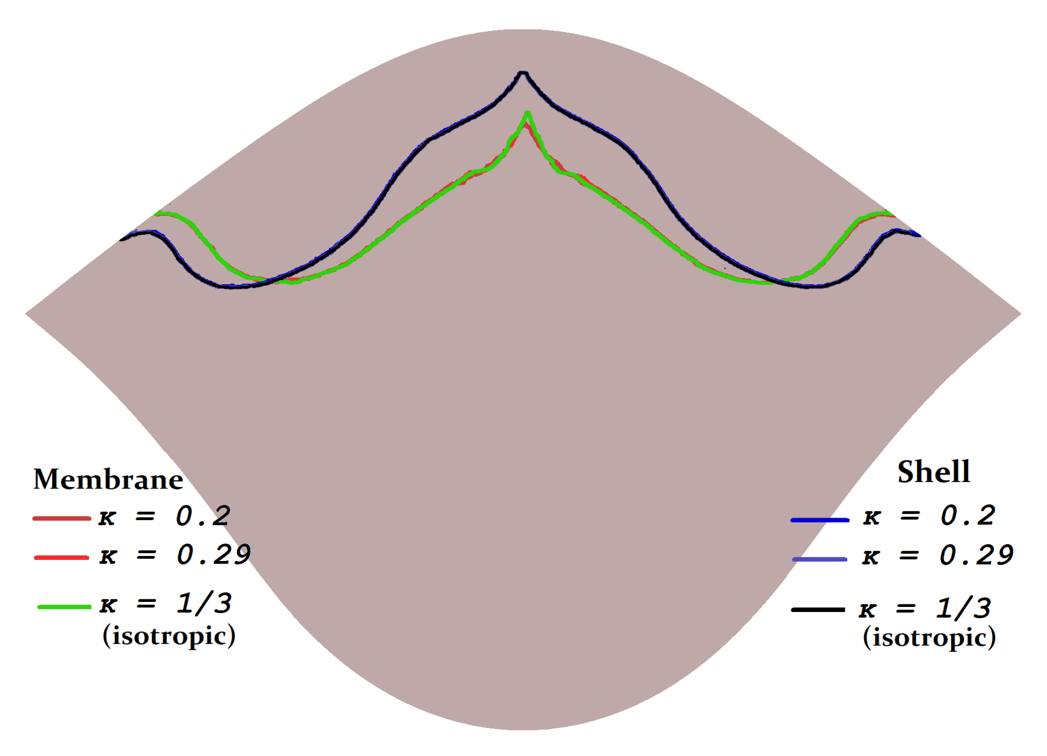
In the scope of one model formulation, the anisotropy degree (variable , Figure 23 and Figure 24) and anisotropy direction (variable , Figure 21 and Figure 22) do not significantly influence the coaptation profile. The results are more notable if we change the model formulation, especially for stiffer material ( kPa). In all the considered cases, the shell formulation reduces the coaptation area and lengthens the coaptation zone along the free edge.
4. Discussion
Both the competence of the reconstructed aortic valves and design leaflet optimization rely on the coaptation characteristics and diastolic valve configuration. These characteristics can be evaluated by the shell or membrane formulations. Some authors insist that “in-plane and flexural mechanical properties of the leaflets play an important role in the valvular function” [33] and thus, one should use the shell formulation. Others suggest that the membrane is a feasible approximation: “we model the native leaflets and pericardium as membranes, assuming negligible flexural stiffness. This is supported by data showing bending stresses at least an order of magnitude smaller than in-plane stresses” [29]. For surgical neocuspidization planning, the membrane formulation is more preferable since it is easy to solve. However, it has to be validated by physical experiments. Moreover, the lack of solid knowledge on the mechanical properties of glutaraldehyde-treated human pericardium hampers the implementation of numerical models in clinical practice.
In our study, we want to explore how the reduced (shell/membrane) model and the leaflet material affects the coaptation zone and the diastolic configuration of the aortic valve. Additionally, we propose a method to compute the leaflet initial configuration, mimicking the real sutured neo-leaflet.
According to our results, the coaptation characteristics are sensitive to the model formulation, especially for stiff materials. The coaptation heights difference is larger (up to 1–2 mm) in the central zone of coaptation. The shell formulation provides usually a lesser coaptation zone than the membrane formulation. A discrepancy of 1–2 mm may be of the order of the central coaptation height. The future leaflet design optimization procedure should account for such a discrepancy. The area of the coaptation zone based on shell formulation is less than that based on membrane formulation: the difference for soft materials ( kPa) is up to and for stiff materials ( kPa) is up to .
Anisotropy of the leaflet material does not affect significantly the coaptation characteristics; this result is similar to that of [28]. Anisotropy can impact the deformed leaflet configuration and produce smaller displacement. For some anisotropy directions, the displacement of the free edge and the belly region are significantly smaller compared to the isotopic case; this result agrees with similar findings for the pulmonary valve [37]. The material stiffness does influence the coaptation zone: it is smaller for stiffer material. Therefore, the study of mechanical properties of the treated human pericardium is highly demanded.
The limitation of our study is using contact planes instead of true leaflets contact, which reduces the computational complexity. Due to the symmetry, it is believed that the results would not change if one considers coaptation of all three leaflets. Validation of our mathematical models by physical experiments is to be performed. This is related to our future work.
Author Contributions
Conceptualization, V.S., A.L. and P.K.; methodology, V.S. and A.L.; software, A.L.; investigation, V.S. and A.L.; draft preparation, V.S., A.L. and P.K. All authors have read and agreed to the published version of the manuscript.
Funding
The study was performed at Marchuk Institute of Numerical Mathematics RAS and was supported by the Russian Science Foundation (project 21-71-30023).
Institutional Review Board Statement
Not applicable.
Informed Consent Statement
Not applicable.
Data Availability Statement
Data and codes are available on request.
Conflicts of Interest
The authors declare no conflict of interest.
References
- Osnabrugge, R.L.J.; Mylotte, D.; Head, S.J.; Van Mieghem, N.M.; Nkomo, V.T.; LeReun, C.M.; Bogers, A.J.J.C.; Piazza, N.; Kappetein, A.P. Aortic stenosis in the elderly: Disease prevalence and number of candidates for transcatheter aortic valve replacement: A meta-analysis and modeling study. J. Am. Coll. Cardiol. 2013, 62, 1002–1012. [Google Scholar] [CrossRef] [PubMed] [Green Version]
- Du, Y.; Gössl, M.; Garcia, S.; Enriquez-Sarano, M.; Cavalcante, J.L.; Bae, R.; Hashimoto, G.; Fukui, M.; Lopes, B.; Ahmed, A.; et al. Natural history observations in moderate aortic stenosis. BMC Cardiovasc. Disord. 2021, 21, 1–10. [Google Scholar] [CrossRef] [PubMed]
- Lowenstern, A.; Sheridan, P.; Wang, T.Y.; Boero, I.; Vemulapalli, S.; Thourani, V.H.; Leon, M.B.; Peterson, E.D.; Brennan, J.M. Sex disparities in patients with symptomatic severe aortic stenosis. Am. Heart J. 2021, 237, 116–126. [Google Scholar] [CrossRef] [PubMed]
- Ando, T.; Onishi, T.; Kuno, T.; Briasoulis, A.; Takagi, H.; Grines, C.L.; Hatori, K.; Tobaru, T.; Malik, A.H.; Ahmad, H. Transcatheter versus surgical aortic valve replacement in the United States (from the Nationwide Readmission Database). Am. J. Cardiol. 2021, 148, 110–115. [Google Scholar] [CrossRef]
- Head, S.J.; Çelik, M.; Kappetein, A.P. Mechanical versus bioprosthetic aortic valve replacement. Eur. Heart J. 2017, 38, 2183–2191. [Google Scholar] [CrossRef]
- Kiyose, A.T.; Suzumura, E.A.; Laranjeira, L.; Buehler, A.M.; Santo, J.A.E.; Berwanger, O.; de Camargo Carvalho, A.C.; de Paola, A.A.; Moises, V.A.; Cavalcanti, A.B. Comparison of biological and mechanical prostheses for heart valve surgery: A systematic review of randomized controlled trials. Arq. Bras. Cardiol. 2019, 112, 292–301. [Google Scholar] [CrossRef]
- Korteland, N.M.; Etnel, J.R.G.; Arabkhani, B.; Mokhles, M.M.; Mohamad, A.; Roos-Hesselink, J.W.; Bogers, A.J.J.C.; Takkenberg, J.J.M. Mechanical aortic valve replacement in non-elderly adults: Meta-analysis and microsimulation. Eur. Heart J. 2017, 38, 3370–3377. [Google Scholar] [CrossRef]
- Rodríguez-Caulo, E.A.; Blanco-Herrera, O.R.; Berastegui, E.; Arias-Dachary, J.; Souaf-Khalafi, S.; Parody-Cuerda, G.; Laguna, G. Biological versus mechanical prostheses for aortic valve replacement. J. Thorac. Cardiovasc. Surg. 2021. Epub ahead of print. [Google Scholar] [CrossRef]
- Diaz, R.; Hernandez-Vaquero, D.; Alvarez-Cabo, R.; Avanzas, P.; Silva, J.; Moris, C.; Pascual, I. Long-term outcomes of mechanical versus biological aortic valve prosthesis: Systematic review and meta-analysis. J. Thorac. Cardiovasc. Surg. 2019, 158, 706–714. [Google Scholar] [CrossRef]
- Zhao, D.F.; Seco, M.; Wu, J.J.; Edelman, J.J.; Wilson, M.K.; Vallely, M.P.; Byrom, M.J.; Bannon, P.G. Mechanical versus bioprosthetic aortic valve replacement in middle-aged adults: A systematic review and meta-analysis. Ann. Thorac. Surg. 2016, 102, 315–327. [Google Scholar] [CrossRef] [Green Version]
- Björk, V.O.; Hultquist, G. Teflon and pericardial aortic valve prosthesis. J. Thorac. Cardiovasc. Surg. 1964, 47, 693–701. [Google Scholar] [CrossRef]
- Love, J.W.; Calvin, J.H.; Phelan, R.F.; Love, C.S. Rapid intraoperative fabrication of an autologous tissue heart valve: A new technique. In Proceedings of the Third International Symposium on Cardiac Bioprostheses, London, UK, 21–23 May 1985; Bodnar, E., Yacoub, M.H., Eds.; Yorke Medical Books: New York, NY, USA, 1986; pp. 691–698. [Google Scholar]
- Ozaki, S.; Kawase, I.; Yamashita, H.; Uchida, S.; Nozawa, Y.; Matsuyama, T.; Takatoh, M.; Hagiwara, S. Aortic valve reconstruction using self-developed aortic valve plasty system in aortic valve disease. Interact. Cardiovasc. Thorac. Surg. 2011, 12, 550–553. [Google Scholar] [CrossRef] [Green Version]
- Benedetto, U.; Sinha, S.; Dimagli, A.; Dixon, L.; Stoica, S.; Cocomello, L.; Quarto, C.; Angelini, G.D.; Dandekar, U.; Caputo, M. Aortic valve neocuspidization with autologous pericardium in adult patients: UK experience and meta-analytic comparison with other aortic valve substitutes. Eur. J. -Cardio-Thorac. Surg. 2021, 60, 34–46. [Google Scholar] [CrossRef] [PubMed]
- Thakeb, Y.M.; Sakr, S.; El Sarawy, E.; Salem, A.M. Short-term competency of aortic valve repair in Egyptian patients. J. Card. Surg. 2020, 35, 598–602. [Google Scholar] [CrossRef] [PubMed]
- Iida, Y.; Akiyama, S.; Shimura, K.; Fujii, S.; Hashimoto, C.; Mizuuchi, S.; Arizuka, Y.; Nishioka, M.; Shimura, N.; Moriyama, S.; et al. Comparison of aortic annulus dimensions after aortic valve neocuspidization with those of normal aortic valve using transthoracic echocardiography. Eur. J. -Cardio-Thorac. Surg. 2018, 54, 1081–1084. [Google Scholar] [CrossRef] [PubMed] [Green Version]
- Siondalski, P.; Wilczynski, L.; Rogowski, J.; Zembala, M. Human aortic bioprosthesis. Eur. J. -Cardio-Thorac. Surg. 2008, 6, 1268. [Google Scholar] [CrossRef] [PubMed]
- Muller, W.H.J.; Warren, W.D.; Dammann, J.F.J.; Beckwith, J.R.; Wood, J.E., Jr. Surgical relief of aortic insufficiency by direct operation on the aortic valve. Circulation 1960, 21, 587–597. [Google Scholar] [CrossRef] [PubMed] [Green Version]
- Tada, N.; Tanaka, N.; Abe, K.; Hata, M. Transcatheter aortic valve implantation after aortic valve neocuspidization using autologous pericardium: A case report. Eur. Heart-J.-Case Rep. 2019, 3, ytz105. [Google Scholar] [CrossRef] [PubMed] [Green Version]
- Hayama, H.; Suzuki, M.; Hashimoto, G.; Makino, K.; Isekame, Y.; Yamashita, H.; Ono, T.; Iijima, R.; Hara, H.; Moroi, M.; et al. Early detection of possible leaflet thrombosis after aortic valve neo-cuspidization surgery using autologous pericardium. J. Am. Soc. Echocardiogr. 2018, 31, B62. [Google Scholar]
- Le Polain De Waroux, J.B.; Pouleur, A.C.; Robert, A.; Pasquet, A.; Gerber, B.L.; Noirhomme, P.; Khoury, G.E.; Vanoverschelde, J.-L.J. Mechanisms of recurrent aortic regurgitation after aortic valve repair: Predictive value of intraoperative transesophageal echocardiography. JACC Cardiovasc. Imaging 2009, 2, 931–939. [Google Scholar] [CrossRef] [Green Version]
- Kunihara, T.; Aicher, D.; Rodionycheva, S.; Groesdonk, H.V.; Langer, F.; Sata, F.; Schäfers, H.J. Preoperative aortic root geometry and postoperative cusp configuration primarily determine long-term outcome after valve-preserving aortic root repair. J. Thorac. Cardiovasc. Surg. 2012, 143, 1389–1395. [Google Scholar] [CrossRef] [Green Version]
- Miyahara, S.; Omura, A.; Sakamoto, T.; Nomura, Y.; Inoue, T.; Minami, H.; Okada, K.; Okita, Y. Impact of postoperative cusp configuration on midterm durability after aortic root reimplantation. J. Heart Valve Dis. 2013, 22, 509–516. [Google Scholar]
- Ridley, C.; Sohmer, B.; Vallabhajosyula, P.; Augoustides, J.G.T. Aortic leaflet billowing as a risk factor for repair failure after aortic valve repair. J. Cardiothorac. Vasc. Anesth. 2017, 31, 1001–1006. [Google Scholar] [CrossRef]
- Schäfers, H.-J.; Bierbach, B.; Aicher, D. A new approach to the assessment of aortic cusp geometry. J. Thorac. Cardiovasc. Surg. 2006, 132, 436–438. [Google Scholar] [CrossRef] [Green Version]
- Li, K.; Sun, W. Simulated transcatheter aortic valve deformation: A parametric study on the impact of leaflet geometry on valve peak stress. Int. J. Numer. Methods Biomed. Eng. 2017, 33, e02814. [Google Scholar] [CrossRef] [Green Version]
- Travaglino, S.; Murdock, K.; Tran, A.; Martin, C.; Liang, L.; Wang, Y.; Sun, W. Computational optimization study of transcatheter aortic valve leaflet design using porcine and bovine leaflets. J. Biomech. Eng. 2020, 142, 011007. [Google Scholar] [CrossRef]
- Loerakker, S.; Argento, G.; Oomens, C.W.; Baaijens, F.P. Effects of valve geometry and tissue anisotropy on the radial stretch and coaptation area of tissue-engineered heart valves. J. Biomech. 2013, 46, 1792–1800. [Google Scholar] [CrossRef] [PubMed] [Green Version]
- Hammer, P.E.; Chen, P.C.; Pedro, J.; Howe, R.D. Computational model of aortic valve surgical repair using grafted pericardium. J. Biomech. 2012, 45, 1199–1204. [Google Scholar] [CrossRef] [PubMed] [Green Version]
- Zakerzadeh, R.; Hsu, M.C.; Sacks, M.S. Computational methods for the aortic heart valve and its replacements. Expert Rev. Med. Devices 2017, 14, 849–866. [Google Scholar] [CrossRef]
- Auricchio, F.; Conti, M.; Ferrara, A.; Morganti, S.; Reali, A. Patient-specific simulation of a stentless aortic valve implant: The impact of fibres on leaflet performance. Comput. Methods Biomech. Biomed. Eng. 2014, 17, 277–285. [Google Scholar] [CrossRef] [PubMed]
- Sun, W.; Abad, A.; Sacks, M.S. Simulated bioprosthetic heart valve deformation under quasi-static loading. J. Biomech. Eng. 2005, 127, 905–914. [Google Scholar] [CrossRef]
- Kim, H.; Lu, J.; Sacks, M.S.; Chandran, K.B. Dynamic simulation of bioprosthetic heart valves using a stress resultant shell model. Ann. Biomed. Eng. 2008, 36, 262–275. [Google Scholar] [CrossRef] [PubMed]
- Smuts, A.N.; Blaine, D.C.; Scheffer, C.; Weich, H.; Doubell, A.F.; Dellimore, K.H. Application of finite element analysis to the design of tissue leaflets for a percutaneous aortic valve. J. Mech. Behav. Biomed. Mater. 2011, 4, 85–98. [Google Scholar] [CrossRef] [PubMed]
- Morganti, S.; Auricchio, F.; Benson, D.J.; Gambarin, F.I.; Hartmann, S.; Hughes, T.J.R.; Reali, A. Patient-specific isogeometric structural analysis of aortic valve closure. Comput. Methods Appl. Mech. Eng. 2015, 284, 508–520. [Google Scholar] [CrossRef]
- Vassilevski, Y.; Liogky, A.; Salamatova, V. Application of Hyperelastic Nodal Force Method to Evaluation of Aortic Valve Cusps Coaptation: Thin Shell vs. Membrane Formulations. Mathematics 2021, 9, 1450. [Google Scholar] [CrossRef]
- Fan, R.; Bayoumi, A.S.; Chen, P.; Hobson, C.M.; Wagner, W.R.; Mayer, J.E., Jr.; Sacks, M.S. Optimal elastomeric scaffold leaflet shape for pulmonary heart valve leaflet replacement. J. Biomech. 2013, 46, 662–669. [Google Scholar] [CrossRef] [Green Version]
- Hofferberth, S.C.; Baird, C.W.; Hoganson, D.M.; Quinonez, L.G.; Emani, S.M.; Pedro, J.; Hammer, P.E. Mechanical properties of autologous pericardium change with fixation time: Implications for valve reconstruction. Semin. Thorac. Cardiovasc. Surg. 2019, 31, 852–854. [Google Scholar] [CrossRef]
- Aguiari, P.; Fiorese, M.; Iop, L.; Gerosa, G.; Bagno, A. Mechanical testing of pericardium for manufacturing prosthetic heart valves. Interact. Cardiovasc. Thorac. Surg. 2016, 22, 72–84. [Google Scholar] [CrossRef] [PubMed] [Green Version]
- Ozolins, V.; Ozolanta, I.; Smits, L.; Lacis, A.; Kasyanov, V. Biomechanical Properties of Glutaraldehyde Treated Human Pericadium. In IFMBE Proceedings, Volume 20, Proceedings of the 14th Nordic-Baltic Conference on Biomedical Engineering and Medical Physics, Riga, Latvia, 16–20 June 2008; Katashev, A., Dekhtyar, Y., Spigulis, J., Eds.; Springer: Berlin/Heidelberg, Germany, 2008; pp. 143–145. [Google Scholar]
- Zigras, T.C. Biomechanics of Human Pericardium: A Comparative Study of Fresh and Fixed Tissue. Ph.D. Thesis, McGill University, Montreal, QC, Canada, 2007. [Google Scholar]
- Salamatova, V.Y.; Liogky, A.A. Method of Hyperelastic Nodal Forces for Deformation of Nonlinear Membranes. Differ. Equ. 2020, 56, 950–958. [Google Scholar] [CrossRef]
- Pavan, P.G.; Pachera, P.; Tiengo, C.; Natali, A.N. Biomechanical behavior of pericardial human tissue: A constitutive formulation. Proc. Inst. Mech. Eng. Part J. Eng. Med. 2014, 228, 926–934. [Google Scholar] [CrossRef]
- Abbasi, M.; Barakat, M.S.; Dvir, D.; Azadani, A.N. A non-invasive material characterization framework for bioprosthetic heart valves. Ann. Biomed. Eng. 2019, 47, 97–112. [Google Scholar] [CrossRef]
- Tepole, A.B.; Kabaria, H.; Bletzinger, K.U.; Kuhl, E. Isogeometric Kirchhoff—Love shell formulations for biological membranes. Comput. Methods Appl. Mech. Eng. 2015, 293, 328–347. [Google Scholar] [CrossRef] [PubMed] [Green Version]
- Oñate, E.; Flores, F.G. Advances in the formulation of the rotation-free basic shell triangle. Comput. Methods Appl. Mech. Eng. 2005, 194, 2406–2443. [Google Scholar] [CrossRef]
- Holzapfel, G. Nonlinear Solid Mechanics: A Continuum Approach for Engineering Science; John Wiley & Sons Ltd.: Chichester, UK, 2000; p. 470. [Google Scholar]
- Holzapfel, G.A.; Ogden, R.W.; Sherifova, S. On fibre dispersion modelling of soft biological tissues: A review. Proc. R. Soc. A 2019, 475, 20180736. [Google Scholar] [CrossRef] [PubMed] [Green Version]
- Lu, J.; Zhou, X.; Raghavan, M.L. Inverse method of stress analysis for cerebral aneurysms. Biomech. Model. Mechanobiol. 2008, 7, 477–486. [Google Scholar] [CrossRef] [PubMed]
- Roohbakhshan, F.; Duong, T.X.; Sauer, R.A. A projection method to extract biological membrane models from 3D material models. J. Mech. Behav. Biomed. Mater. 2016, 58, 90–104. [Google Scholar] [CrossRef] [PubMed]
- Ciarlet, P.G. Mathematical Elasticity. Volume I: Three-Dimensional Elasticity; Publishing House: Amsterdam, The Netherlands, 1988; p. 451. [Google Scholar]
- User Documentation for KINSOL v5.7.0 (SUNDIALS v5.7.0). Available online: https://computing.llnl.gov/sites/default/files/kin_guide.pdf (accessed on 7 September 2021).
- Terekhov, K.M.; Konshin, I.N.; Vassilevski, Y.V.; Danilov, A.A. Parallel software platform INMOST: A framework for numerical modeling. Supercomput. Front. Innov. 2016, 2, 55–66. [Google Scholar]
- Baird, C.W.; Marathe, S.P.; Pedro, J. Aortic valve neo-cuspidation using the Ozaki technique for acquired and congenital disease: Where does this procedure currently stand? Indian J. Thorac. Cardiovasc. Surg. 2020, 36, 113–122. [Google Scholar] [CrossRef]
Figure 1.
Pipeline for constructing sutured leaflet.
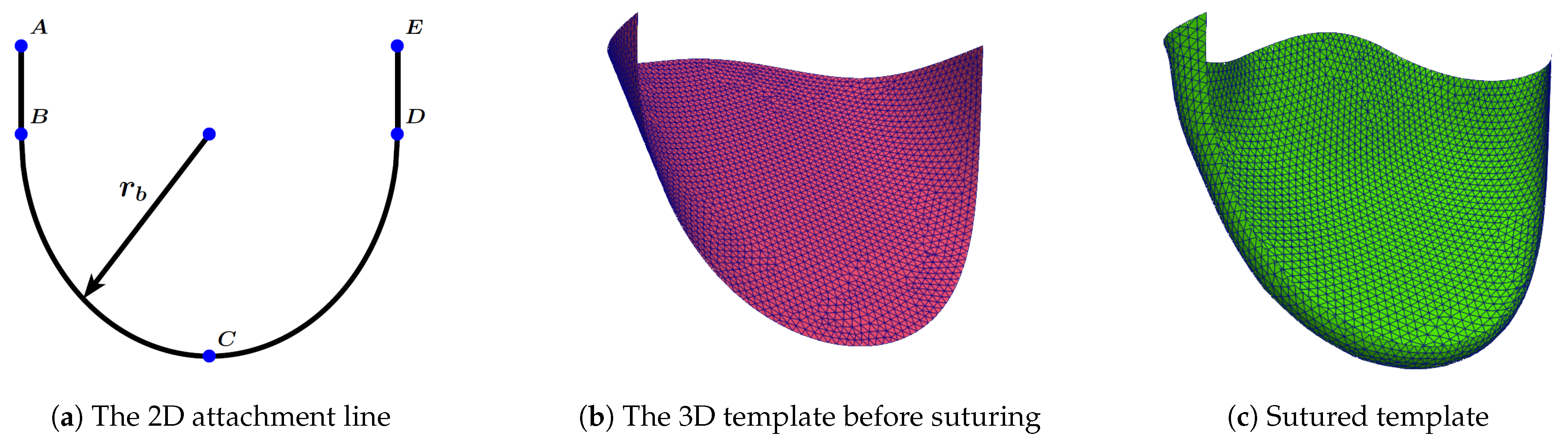
Figure 2.
Attachment line on a plane.
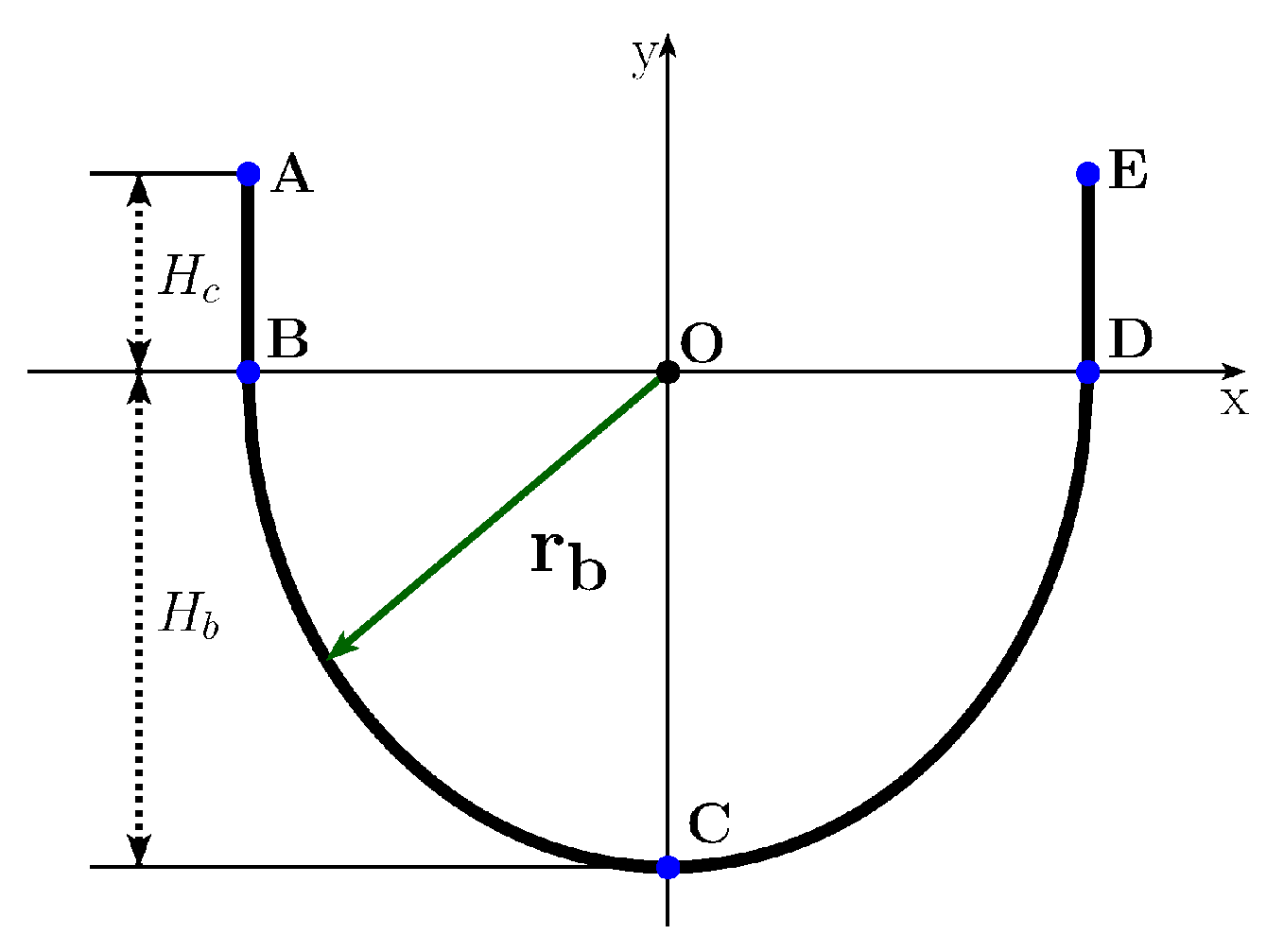
Figure 3.
Attachment line on a cylinder.
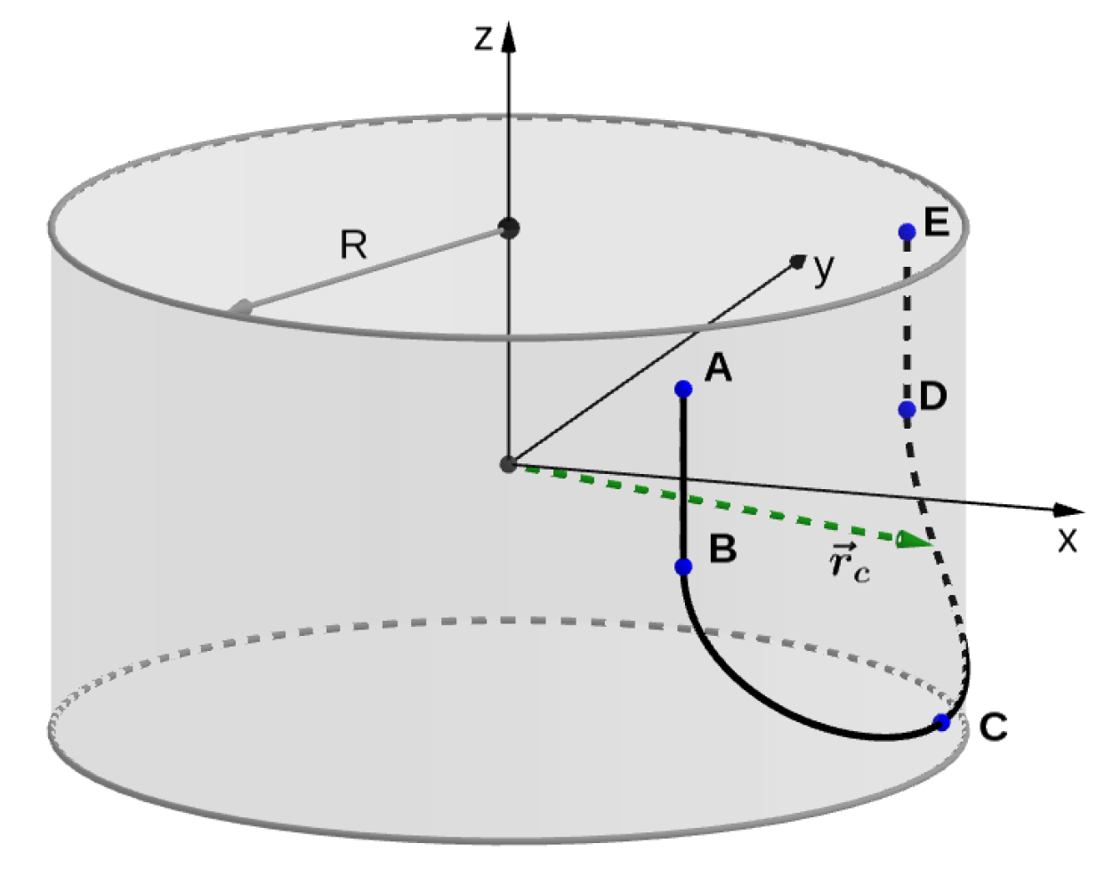
Figure 4.
The 3D leaflet template before suturing.
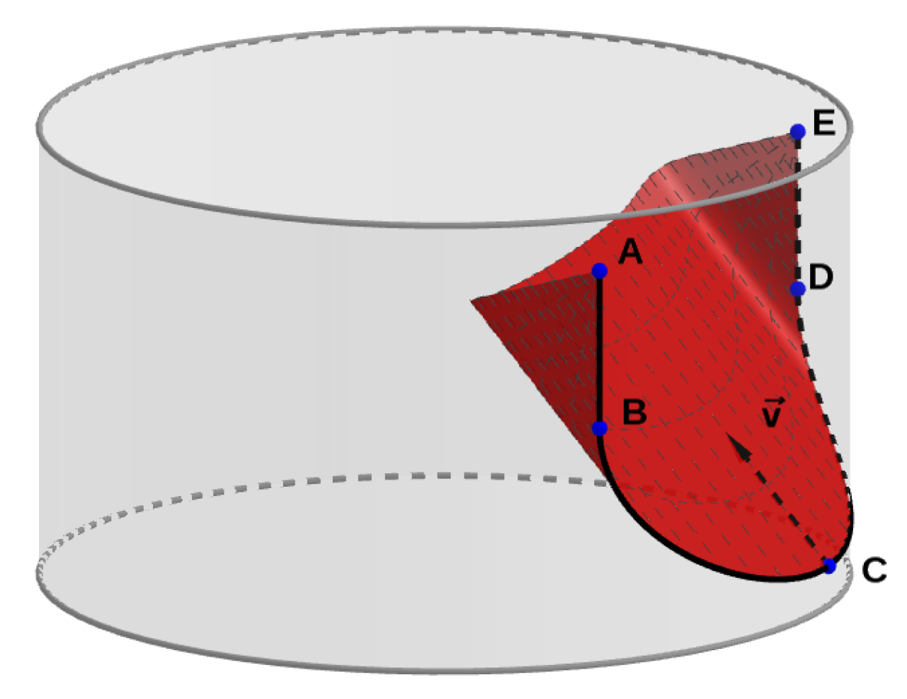
Figure 5.
(a) Deformation of triangle. (b) Patch of elements consisting of the central triangle and three adjacent elements. The figure from [36].
Figure 5.
(a) Deformation of triangle. (b) Patch of elements consisting of the central triangle and three adjacent elements. The figure from [36].
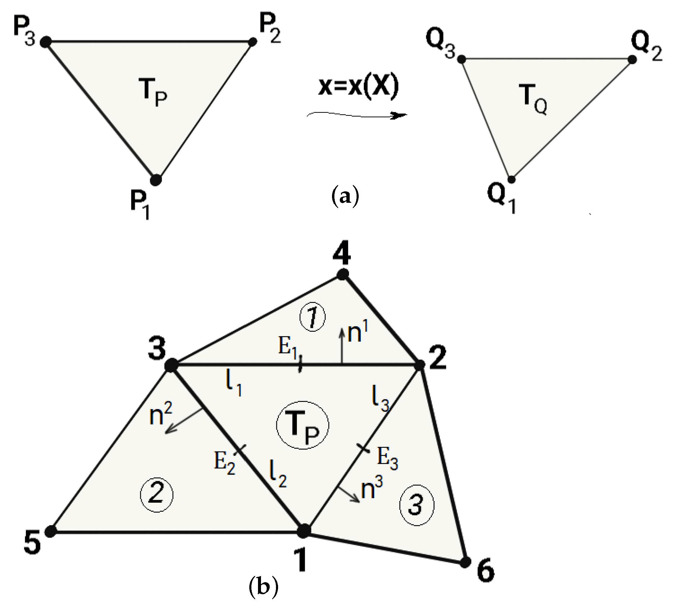
Figure 6.
Sketch for defining the nodal suturing force .
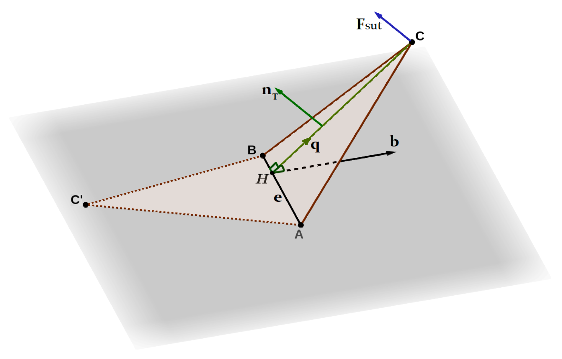
Figure 7.
Dependence of the nodal suturing force on the angle .

Figure 8.
Initial template before suturing (left). Template after suturing (right).
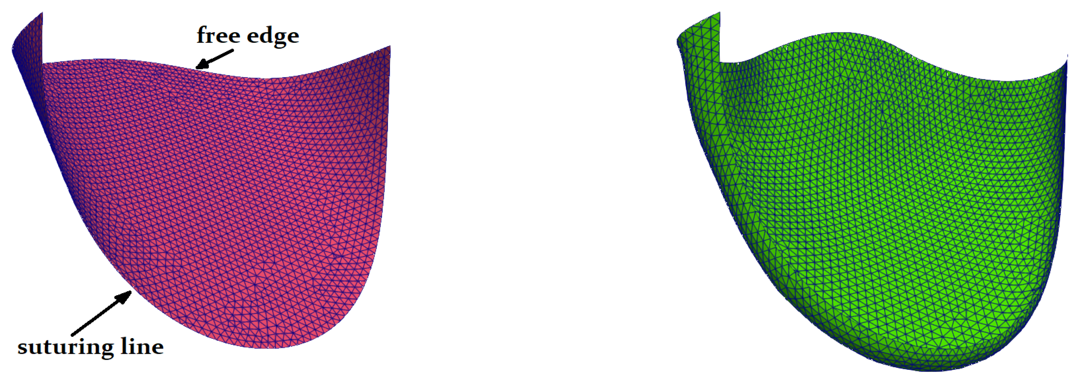
Figure 9.
Schematic representation of contact (penalty) planes by segments , , and . The pink area is the allowed area for the sutured leaflet configuration. In fact, the cylindrical surface is not a constraint, and during the simulation, the template can freely go beyond it.
Figure 9.
Schematic representation of contact (penalty) planes by segments , , and . The pink area is the allowed area for the sutured leaflet configuration. In fact, the cylindrical surface is not a constraint, and during the simulation, the template can freely go beyond it.

Figure 10.
Boundary conditions for leaflet: left contact plane (blue); right contact plane (red); clamped attachment line (black); free edge (green).
Figure 10.
Boundary conditions for leaflet: left contact plane (blue); right contact plane (red); clamped attachment line (black); free edge (green).

Figure 11.
Isotropic, membrane, kPa. Initial configuration (green); deformed configuration (red).
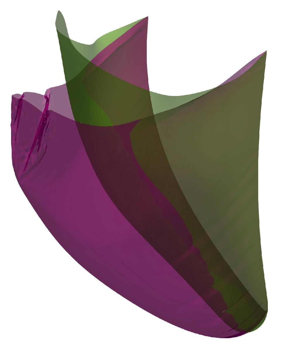
Figure 12.
Isotropic, shell, kPa. Initial configuration (green); deformed configuration (red).
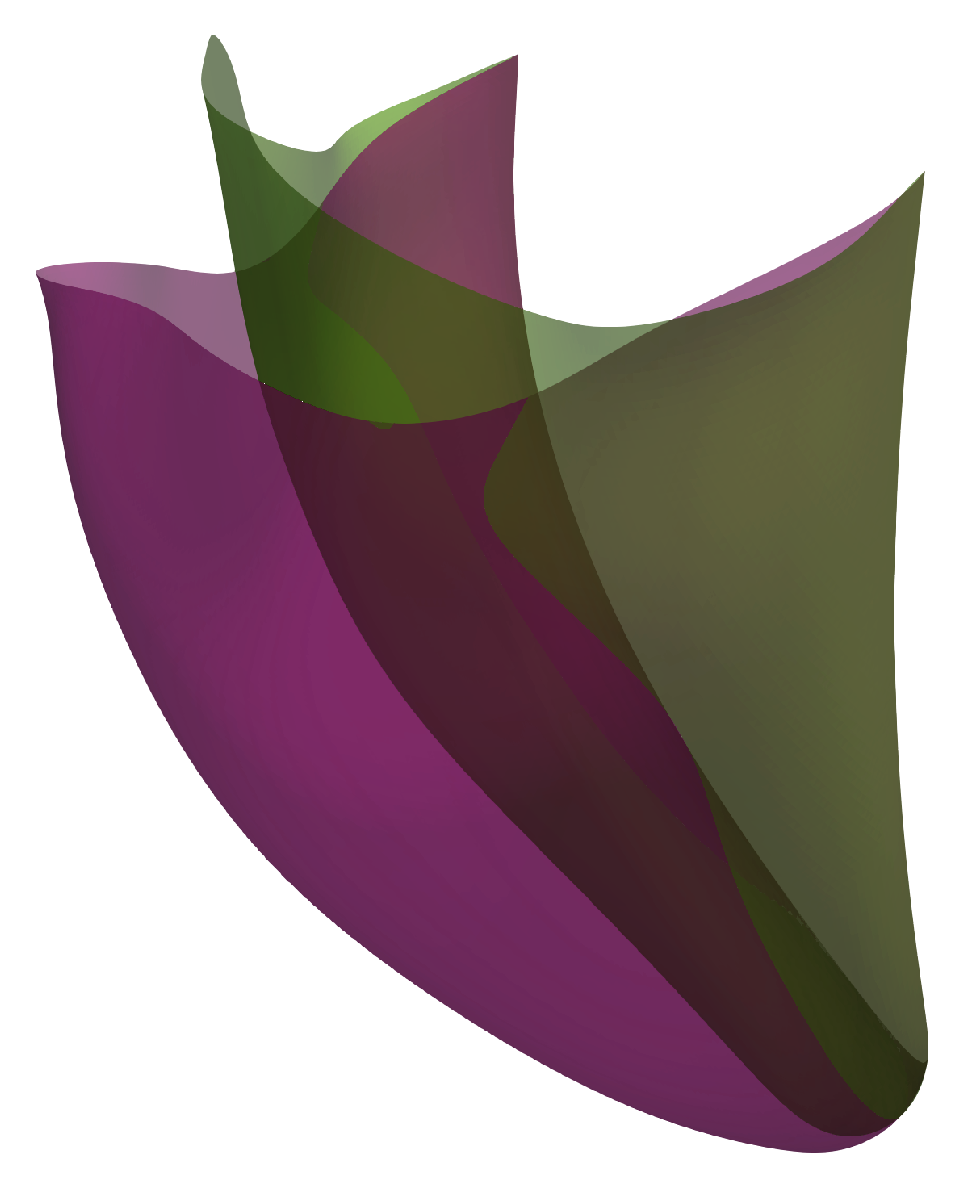
Figure 13.
Anisotropic, kPa, , . Initial configuration (green); deformed shell (red); deformed membrane (blue).
Figure 13.
Anisotropic, kPa, , . Initial configuration (green); deformed shell (red); deformed membrane (blue).
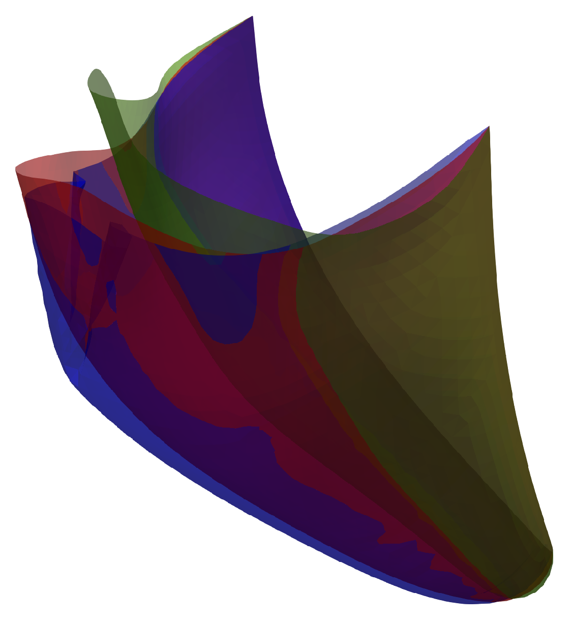
Figure 14.
Anisotropic, kPa, , . Initial configuration (green); deformed shell (red); deformed membrane (blue).
Figure 14.
Anisotropic, kPa, , . Initial configuration (green); deformed shell (red); deformed membrane (blue).
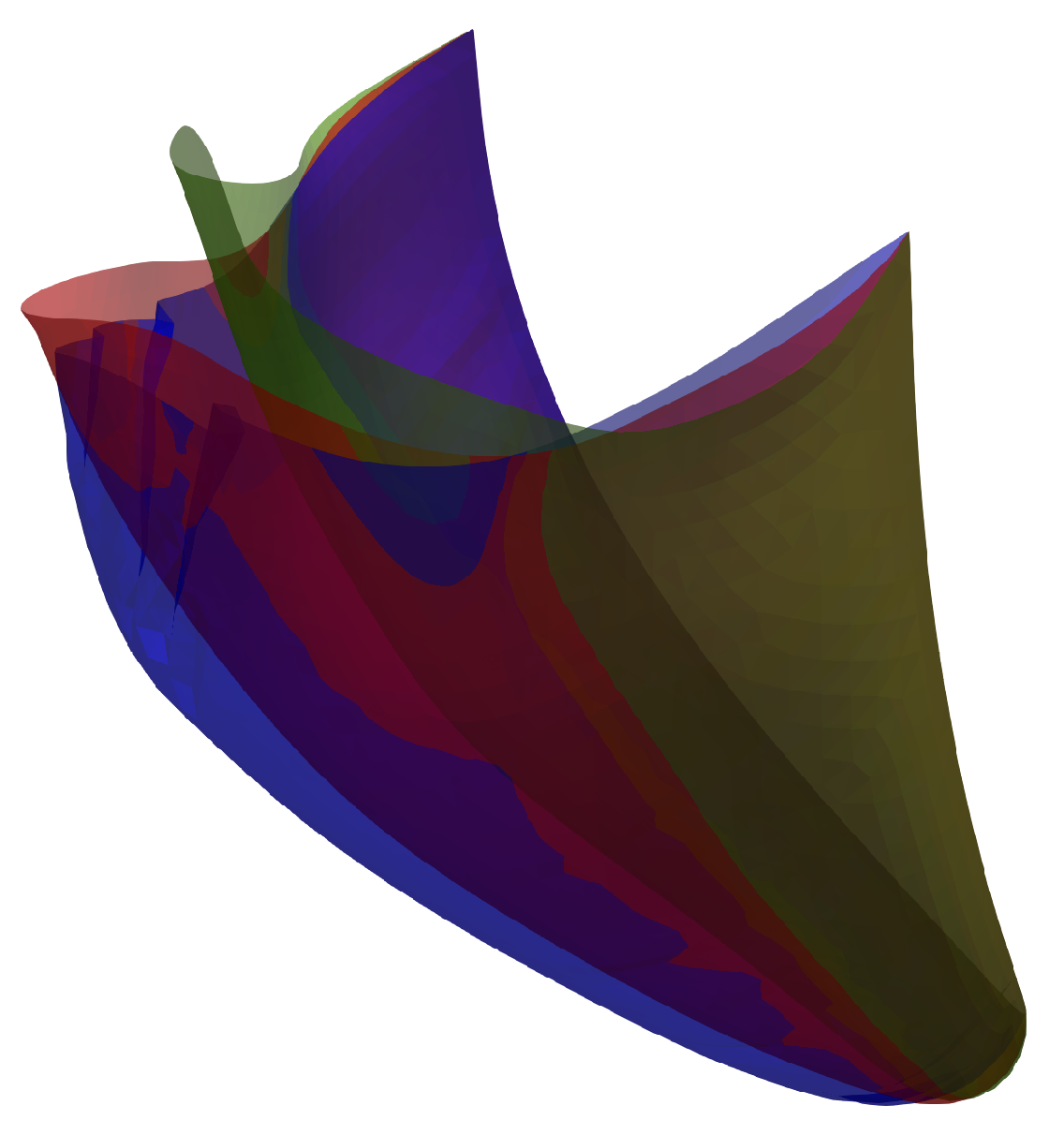
Figure 15.
Membrane, kPa; isotropic (red); anisotropic , (green); anisotropic , (blue).
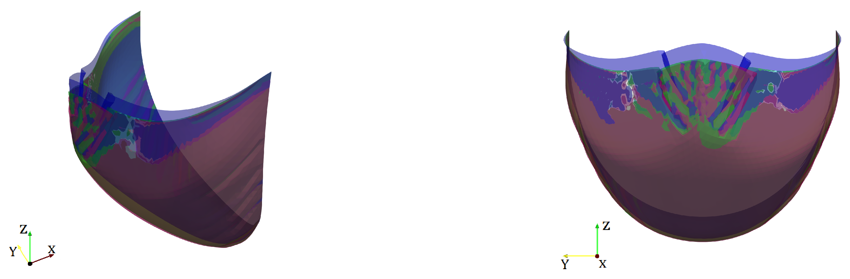
Figure 16.
Shell, kPa; isotropic (red); anisotropic , (green); anisotropic , (blue).
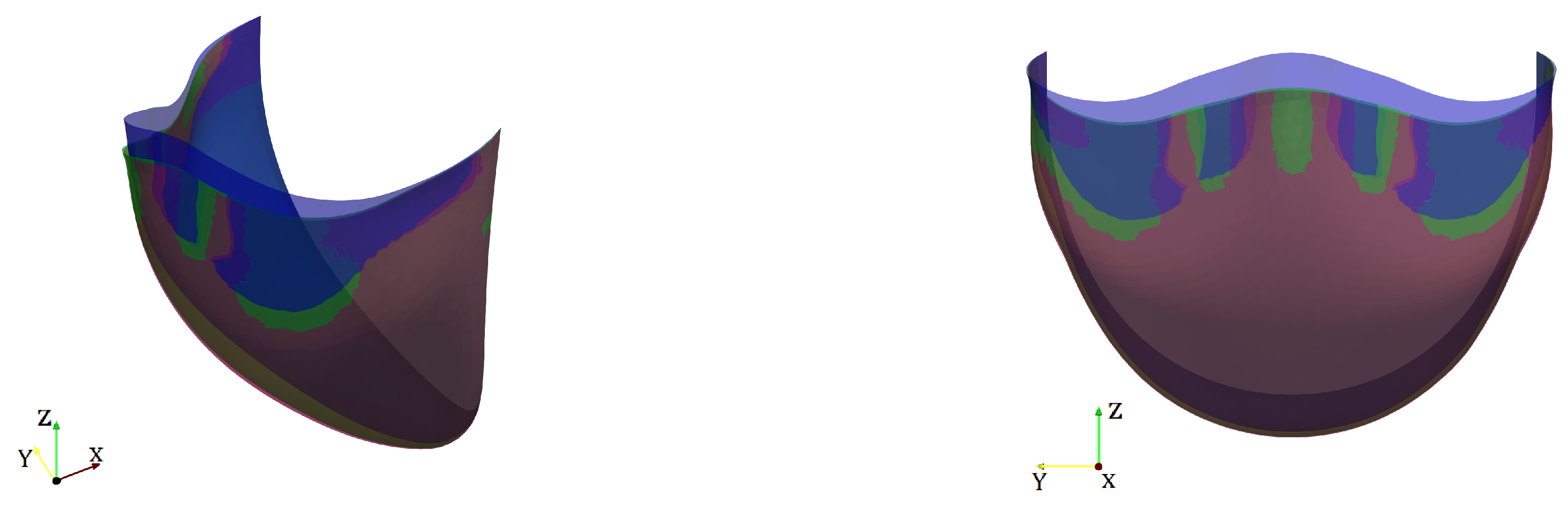
Figure 17.
Membrane, kPa; isotropic (red); anisotropic , (green); anisotropic , (blue).
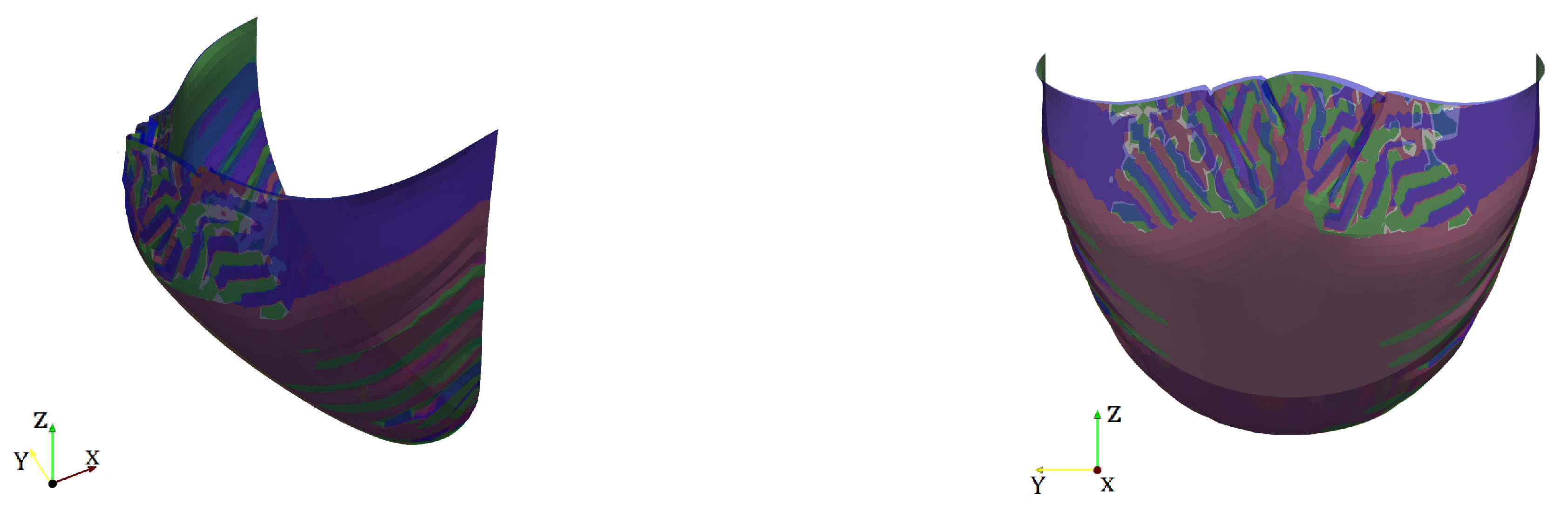
Figure 18.
Shell, kPa; isotropic (red); anisotropic , (green); anistropic , (blue).
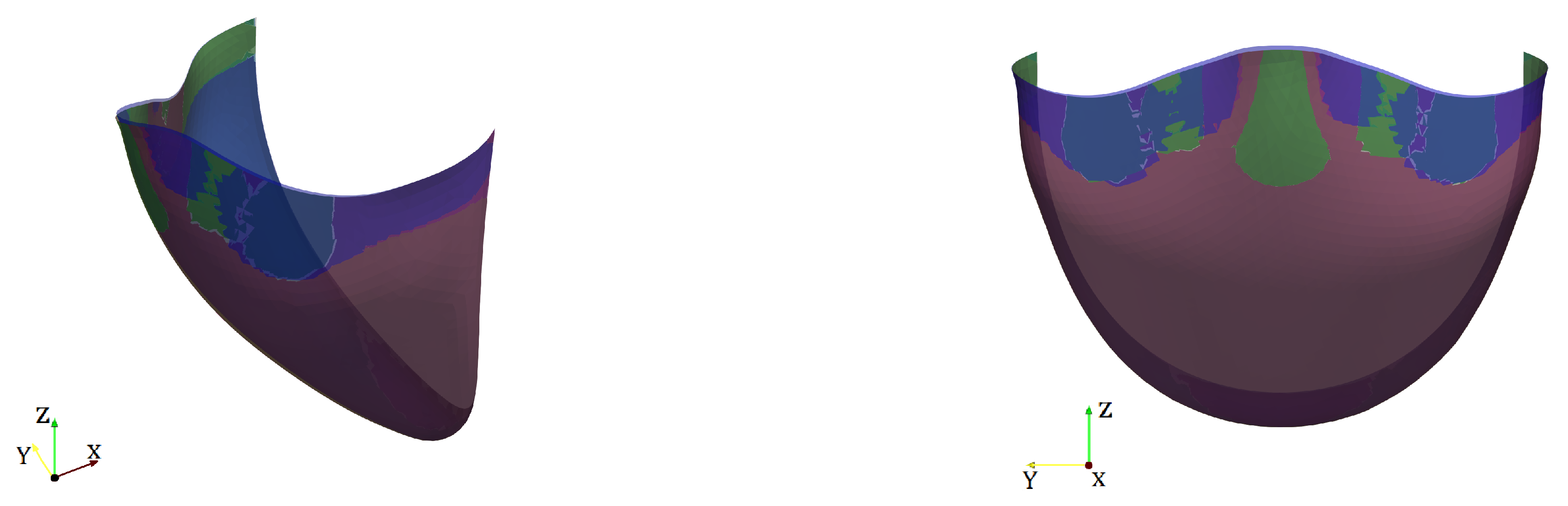
Figure 19.
Coaptation area for different model parameters and model formulations.
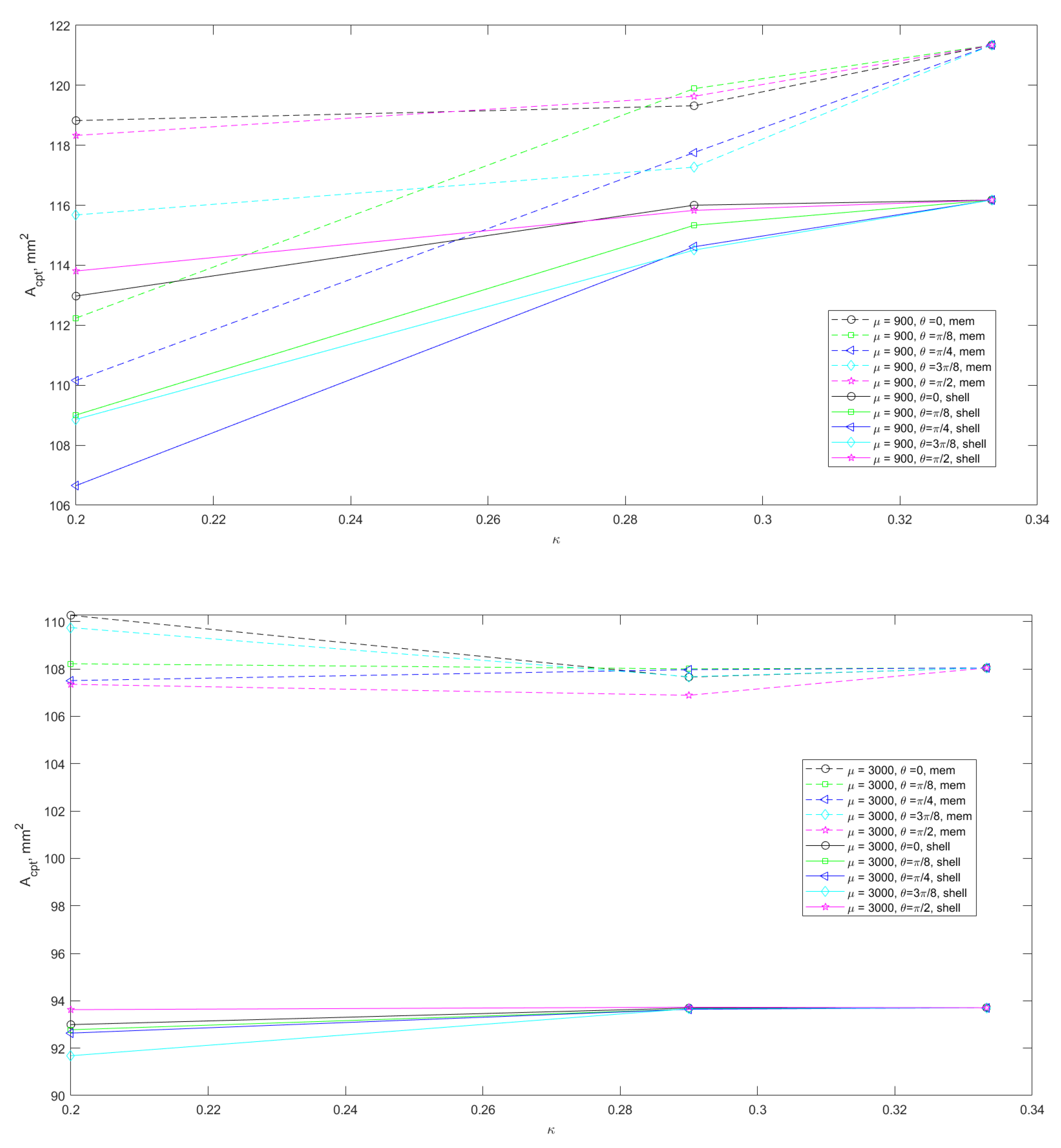
Figure 20.
Difference of coaptation area (membrane-shell) for different model parameters.
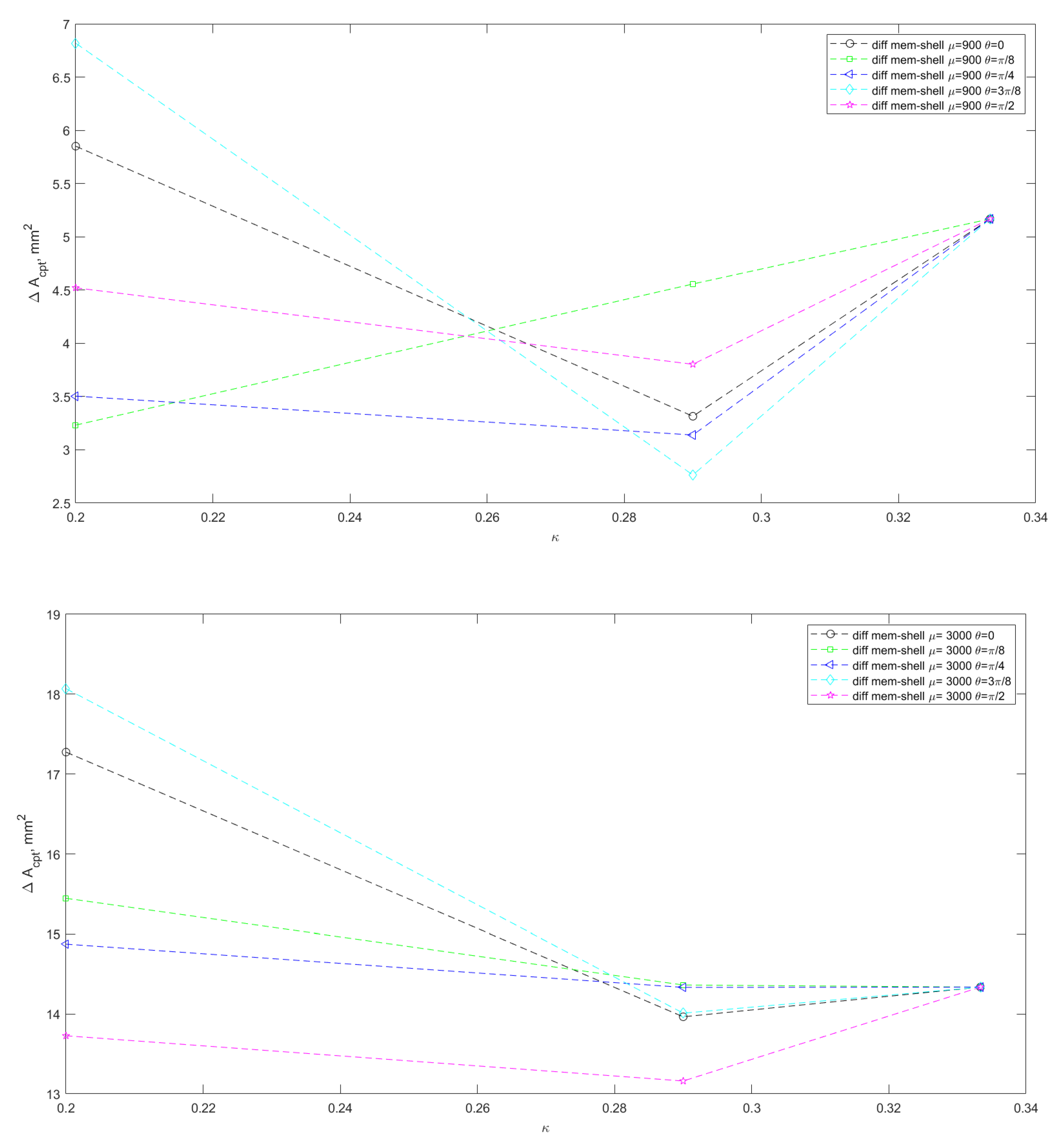
Figure 21.
Coaptation profiles for kPa, , varied on the unfolded template. Profiles for membrane are almost the same except the central zone; profiles for shell are almost the same.
Figure 21.
Coaptation profiles for kPa, , varied on the unfolded template. Profiles for membrane are almost the same except the central zone; profiles for shell are almost the same.

Figure 22.
Coaptation profiles for kPa, , varied on the unfolded template. Profiles for shell are superimposed on each other; profiles for membrane are almost the same.
Figure 22.
Coaptation profiles for kPa, , varied on the unfolded template. Profiles for shell are superimposed on each other; profiles for membrane are almost the same.
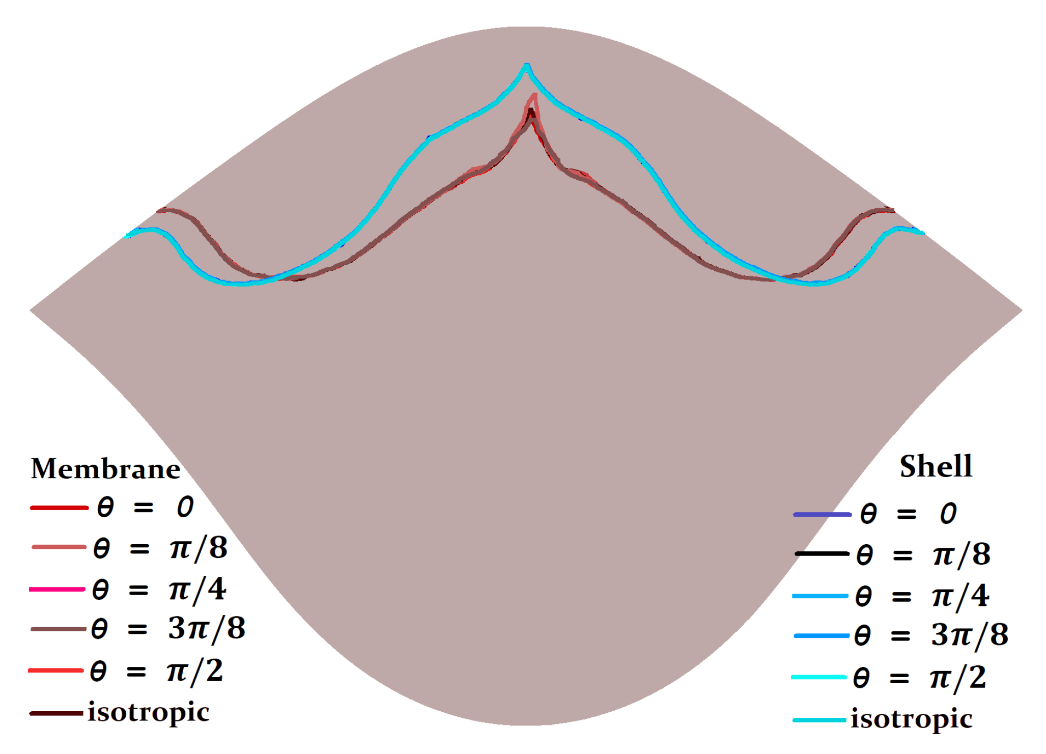
Figure 23.
Coaptation profiles for kPa, , varied on the unfolded template.
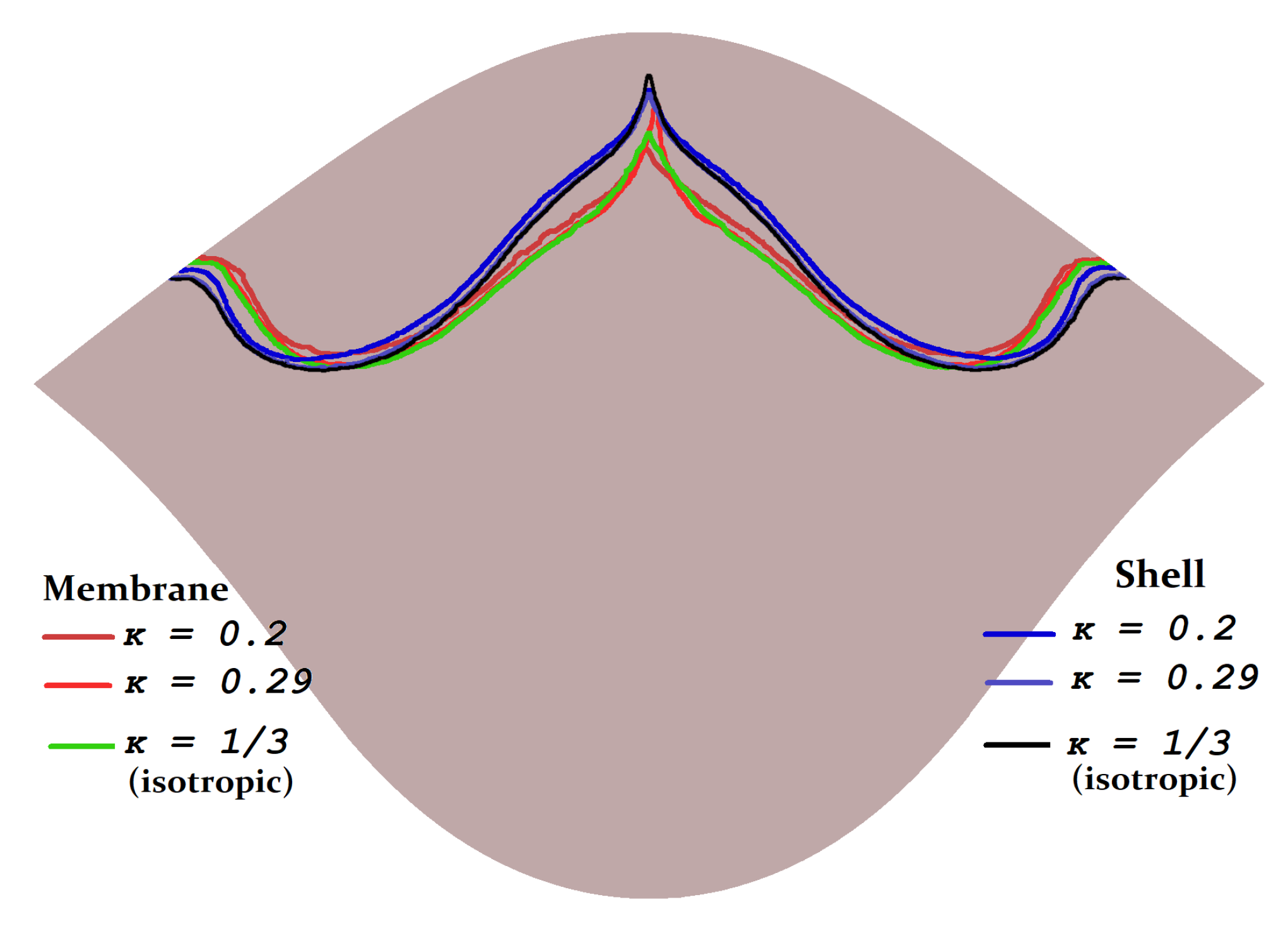
Figure 24.
Coaptation profiles for kPa, , varied on the unfolded template. Profiles for shell are superimposed on each other; profiles for membrane are almost the same.
Figure 24.
Coaptation profiles for kPa, , varied on the unfolded template. Profiles for shell are superimposed on each other; profiles for membrane are almost the same.
Publisher’s Note: MDPI stays neutral with regard to jurisdictional claims in published maps and institutional affiliations. |
© 2021 by the authors. Licensee MDPI, Basel, Switzerland. This article is an open access article distributed under the terms and conditions of the Creative Commons Attribution (CC BY) license (https://creativecommons.org/licenses/by/4.0/).
Share and Cite
MDPI and ACS Style
Liogky, A.; Karavaikin, P.; Salamatova, V. Impact of Material Stiffness and Anisotropy on Coaptation Characteristics for Aortic Valve Cusps Reconstructed from Pericardium. Mathematics 2021, 9, 2193. https://doi.org/10.3390/math9182193
AMA Style
Liogky A, Karavaikin P, Salamatova V. Impact of Material Stiffness and Anisotropy on Coaptation Characteristics for Aortic Valve Cusps Reconstructed from Pericardium. Mathematics. 2021; 9(18):2193. https://doi.org/10.3390/math9182193
Chicago/Turabian StyleLiogky, Alexey, Pavel Karavaikin, and Victoria Salamatova. 2021. "Impact of Material Stiffness and Anisotropy on Coaptation Characteristics for Aortic Valve Cusps Reconstructed from Pericardium" Mathematics 9, no. 18: 2193. https://doi.org/10.3390/math9182193
Note that from the first issue of 2016, this journal uses article numbers instead of page numbers. See further details here.