
Energy Based Calculation of the Second-Order Levitation in Magnetic Fluid


Faculty of Electrical Engineering and Computer Science, University of Maribor, Koroska cesta 46, 2000 Maribor, Slovenia
*
Author to whom correspondence should be addressed.
Mathematics 2021, 9(19), 2507; https://doi.org/10.3390/math9192507
Submission received: 31 August 2021
/
Revised: 27 September 2021
/
Accepted: 4 October 2021
/
Published: 7 October 2021
(This article belongs to the Special Issue Numerical Model and Methods for Magnetic Fluids)
Abstract
:A permanent magnet immersed in magnetic fluid experiences magnetic levitation force which is of the buoyant type. This phenomenon commonly refers to self-levitation or second-order buoyancy. The stable levitation height of the permanent magnet can be attained by numerical evaluation of the force. Various authors have proposed different computational methods, but all of them rely on force formulation. This paper presents an alternative energy approach in the equilibrium height calculation, which was settled on the minimum energy principle. The problem, involving a cylindrical magnet suspended in a closed cylindrical container full of magnetic fluid, was considered in the study. The results accomplished by the proposed method were compared with those of the well-established surface integral method already verified by experiments. The difference in the results gained by both methods appears to be under 2.5%.
1. Introduction
In recent years, many researchers working on problems involving magnetic fluid were focused on the self-levitation phenomenon, which occurs when a permanent magnet (PM) is suspended in magnetic fluid (MF). This phenomenon was first reported by Rosensweig in 1966 [1,2]. A study of the forces acting on such a body has shown that, in addition to the Archimedes buoyancy, another type of buoyancy appears by virtue of the magnetic field. Such force is called a magnetic levitation force (MLF), also known as second-order buoyancy. This new kind of buoyancy is not limited only to the vertical direction, but acts as the restoring force for any displacement of the PM from the stable levitating position.
Because of this, a PM suspended in MF has found many practical applications, the most promising of which are dampers and accelerometers. The first damper of this kind, consisting of PM and MF, was the ferrofluid inertia damper proposed by Moskowitz et al. in 1978, designed to operate in the self-levitated condition [3]. Later on, the configuration was improved to achieve better performances, but the basic concept remained unchanged [4,5]. The passive ferrofluid dynamic vibration absorber presented in [6] is also a damping device based on the self-levitation phenomenon. Such an absorber is used to suppress small amplitude (<1 mm) and low-frequency vibrations (<1 Hz). Some modifications to the beforementioned absorber have been disclosed in [7]. For more recent theoretical and experimental studies on the ferrofluid dynamic vibration absorbers, the readers may refer to [8,9].
Another interesting and promising application that works on the self-levitation principle is the magnetic fluid-based accelerometer. The typical design of such a device, presented in [10], is similar to the one introduced with the dampers, but here the inductive coil is mounted over the housing to detect the PM movement. In the past few years, the magnetic liquid-based accelerometers have been researched intensively due to their relatively simple and reliable design [11,12]. Almost all the relevant publications in the field were provided by the research groups from China, where the topic of second-order buoyancy has been addressed both theoretically and experimentally. Yang et al. [13] calculated the magnetic self-levitation force of a cylindrical PM with the use of the magnetic charge image method and current image method, respectively. Results have shown a large difference of up to 62% between the calculated and measured results. On the other hand, by employing FEM on the problem the error did not exceed 9%. The same authors continued with research on the radial MLF in the following years [8,14]. The current image method and FEM were employed successfully in the optimization of a magnetic fluid accelerometer [11]. Based on the magnetic field solution obtained by the commercial FEM software, three effective and practical computational methods were proposed in [12]: the surface integral method (SIM), the magnetic force method, and equivalent magnetic force method. The results achieved by the aforementioned methods matched the experimental results within 7%. The experimental setup for measuring MLF involved a non-magnetic rod attached to the top of the PM which influenced the force acting on the PM. The detailed model based on the SIM and the influence of the measuring rod were studied in [15,16]
There were also some research studies devoted to the development of micro magnetic fluid devices for driving micro machines. Here, the PM is coated with MF, which acts as a lubricant. The movement of the PM can be achieved in an alternating magnetic field [17,18].
This article uses two different approaches in calculating the equilibria states of the permanent magnet (PM) immersed in the magnetic fluid (MF). The first approach is based on the force formulation, where the stable magnetic state is calculated through the Surface Integral Method (SIM). This method is well covered, theoretically and experimentally, by various authors [12,15,16,19]. The main reason it appears in the current study is to use it as a benchmark for the proposed method, based on the energy formulation.
To the best of the authors’ knowledge, the self-levitation equilibria of the PM have not been studied by virtue of the energy. To fill this gap in the field, and to illuminate the addressed topic from a different standpoint, a mathematical model grounded on the energy principle is presented in this article. Such a formulation is essential, since numerical issues arise when the SIM is implemented on the first-order finite element mesh [20]. Not going in deep with the error analysis associated with the numerical evaluation of the stress tensor, only a summary on the subject is given here. The mesh size on the contour path should be as fine as possible; the integration should be performed in the free space (air), or at least in a region with a constant permeability; the contour should not be defined at the interface between two different materials, but always a few elements away from any interfaces or boundaries [20,21]. In practical applications, whether the user is coding or just using the FEM-based software, considering the enlisted requirements could represent quite demanding work. Anyhow, when the self-levitation equilibrium is tackled with the energy formulation, the issues mentioned above could be avoided successfully.
2. Materials and Methods
The content of this chapter is devoted to the problem definition, and to introduce the reader to the basic, but still comprehensive, theoretical background. Even though the quite extensive mathematical employment used here could be omitted, as the majority of it can be found in [16], the authors have kept it here on purpose; in the first place, to point out some crucial differences between the existing approaches reported by other authors.
2.1. Problem Definition
Analysis of the self-levitation phenomena associated with a PM immersed in MF depends on the engaged geometry and material properties of the solids and liquids involved [11]. This study is focused on the simple cylindrical geometry, where both the PM and the container with MF are cylindrical. Onward, the PM is placed in a closed and fully filled container in such way that both axes coincide. The basic deployment is shown in Figure 1.
2.2. Surface Integral Method (SIM)
The mathematical expression of the magnetic fluid levitation force (MFLF) which acts on the PM immersed in MF could be derived from magnetic fluid stress tensor proposed by Rosensweig in 1966 [22]. The origin of the force is in the interaction between a permanent magnet’s field and the magnetic liquid’s magnetization. It drags a permanent magnet into the equilibrium state, where the total energy reaches its minimum.
Here, is the surface of the PM; is a unit vector normal to the PM’s surface, pointing outward in the MF (see Figure 2); is a surface element; is the pressure in the MF in the absence of a magnetic field; is the volume of MF per unit mass i.e., where stands for the MF’s density; is the permeability of the free space; is the magnetization of the MF; and are the magnetic flux density in the vector notation and its absolute value, respectively; and are the magnetic field intensity in the vector and its corresponding absolute value, respectively; is an identity matrix; and is the absolute temperature. The product represents a tensor. All the physical quantities stated in Equation (1) and Equation (2) are, in general, functions of position, e.g., , , , , , etc., but a shorter notation was used here for convenience.
Executing a derivation in the square brackets of the above expression at constant and gives
When the fluid is at rest and fully enclosed within the container (there are no free surfaces), the pressure represents the hydrostatic pressure caused by the gravity. To emphasize this, the subscript for the gravity is added to it, i.e., . The notation of Equation (3) is usually written in the following form [22],
where the fluid-magnetic pressure and the magnetostrictive pressure are defined as
In most of the practical cases where the fluid is considered incompressible, the latter term can be omitted from the further analysis, i.e., [22].
Considering the MF equilibrium state with respect to the representation shown in Figure 2, the following equation can be given.
Here, is the surface of the container; is a unit vector normal to the surface , pointing inward to the MF (see Figure 2); is the volume of the MF; is the acceleration vector of gravity; and is a volume element.
Equation (7) gives a balance of the forces in the MF; here, the term on the left side of the equation represents the gravity force of the MF, and the right side stands for the buoyancy force, which consists of magnetic and Archimedes components. The surface exposed to the MF is here indicated with .
Expressing Equation (1) with Equation (7) results in a more propriate formulation of magnetic fluid levitation force [16].
Considering Equations (4)–(6) in Equation (8) a further development follows:
By looking at Equation (9), it can easily be noticed that the first two terms on the right side correspond to the Archimedes buoyancy force . The others terms declare the magnetic contribution to the magnetic fluid levitation force , i.e., .
In the relevant literature, the force also refers to the magnetic levitation force (MLF), the opposite value of which is known as second-order buoyancy . In other words, [15,16,19].
The magnetic part of the second-order buoyancy force, or MLF (), can be calculated by integrating solely over the container’s surface . The numerical evaluation of the second-order buoyancy force in this article, as well as in the research studies conducted in [15], is realized based on the statement given in Equation (12). The conditions are given illustratively in Figure 3; the acts in favor of the PM’s stable position.
Maybe it is not evident at first, but Equation (12) gives a very useful mathematical tool. Namely, while all the physical significance of the interest, i.e., the force , is reflected through the integration over the surface bounding the MF, despite changes inside the boundary. The following illustrative examples shown in Figure 4 should give a transparent understanding of Equation (12). In the first case, labeled by (a) in the Figure, where only a PM is floating inside the liquid, force is obtained by integrating along the four Sections 1–2, 2–3, 3–4, and 4–1. Now, suppose some other object besides PM floats within the MF, as shown in Figure 4b. While the surface of the container is not affected by the additional object, the calculation of force follows the same procedure. If the setup is given as in Figure 4c, where a non-magnetic rod is attached to the PM and passes through the container, then the integration over the rod’s surface in the container’s hole should be included in the force calculation, due to the difference in the magnetic properties of the rod and the MF. The integration pertaining to the MF is performed through the paths 1–5, 6–2, 2–3, 3–4 and 4–1, while Sections 5 and 6 passes through the non-magnetic rod.
A peculiarly interesting case relevant for an experimental verification or a practical application is the one marked by (c) in Figure 4. Here, the non-magnetic rod is attached to the PM at one side, while the other—upper—side goes to a dynamometer not shown in the figure. Because such an arrangement was used in the experiments conducted in [15], the same composition comes with the simulation model presented by the current study.
2.3. Energy Method
It was mentioned in the previous section that the static equilibrium is met when the energy of a physical system under consideration reaches its minimum. In classical physics, this is known as the principle of minimum energy. The principle has its background in thermodynamics, and could be applied prosperously to a wide range of problems involving magnetic fluids, such as magnetocaloric energy conversion and magnetic liquid free surface instabilities [22,23]. Not wishing to enter further into the topic, for the case study presented here, it suffices to consider the total energy as a sum of the gravitational and magnetostatic energy
where is the total energy; and are gravitational potential energy and magnetostatic energy, respectively.
Here, the gravitational energy is given as a function of a PM levitation height, as shown in Figure 5.
A specific gravitational energy, or gravitational energy per unit of volume, can be stated as
Here, and are the density of the PM and MF, respectively; is the difference in material densities; is the PM volume; is the levitation height (see Figure 5); is the density of gravitational energy; and is gravity acceleration. For simplicity, the MF is assumed as a homogeneous media, thus the parameters and could be considered as constants. In reality, the concentration of magnetic nanoparticles is denser in the vicinity of the PM, while the magnetic nanoparticles are attracted toward the region with the higher magnetic field [11].
While the levitation height of the PM is subjected to change, the magnetic field will not be distributed symmetrically with respect to the -axis, and, consequently, the magnetostatic energy density will vary with the position of the PM. To take into account the spatial variation of the energy as well as the MF nonlinear magnetization characteristic, the magnetostatic energy is written as a function of the density of magnetostatic energy as follows,
In the latter equation, and stand for the lower and upper integration limits, and represent the initial and the final fields established in the magnetizing process, respectively. The expression for the magnetostatic energy density given with Equation (17) holds in general for both the linear and nonlinear relations between quantities and . With the linear magnetic conditions, this expression becomes .
The main idea is to find the PM levitation height at which the total energy announced by Equation (13) is minimal. The aforementioned task is not achieved easily without computer-aided numerical methods; after all, knowing the magnetic field distribution in the space is essential to the problem. However, still, with some simplifications applied to the model, the problem can be handled analytically to some extent. The following consideration of the equilibrium state of the PM immersed in an MF is addressed by qualitative rather than quantitative analysis.
Suppose the arrangement as shown in Figure 6, which is unbounded in both and directions. The MF with constant permeability occupies the space from the reference level at to the height of the container at . The space surrounding the MF is free space or air with the permeability . Now, imagine having such a PM which has an infinitesimally small thickness and is extended extensively over the plane at the height within the MF. As indicated in Figure 6, the computational domain is divided into four sections, 1 to 4. Section 1 corresponds to the region with the MF above the PM, Section 3 announces the free space above the PM, and a similar indication is carried out for the regions below the PM, where Section 2 and Section 4 pertain to the MF and free space region below the PM, respectively. The magnetic field intensity and magnetic flux density at the PM’s surface are and , respectively, which are specified by the PM’s properties. Assuming the edges of the PM are distant from the segment of interest, then a -component of a magnetic field will dominate near that fraction of the PM. To the first approximation, an exponential decrease in the magnetic field can be assumed with respect to the vertical distance from the piece of the PM in question. The rate of change in the field is determined by another PM’s constant, . Here, the levitation height of the PM is indicated with and is taken as a parameter.
The relation between and in the matter can be written in a particularly useful form when the medium has a constant permeability
According to Figure 6, the magnetic field intensity in the MF’s region above the PM in region 1, , is stated with Equation (20).
Applying Equation (19) to Equation (20) gives a magnetic flux density in region 1
At this point, it is appreciated to assert a total differential of with respect to , which appears in the expression for the density of magnetostatic energy in Equation (17)
where corresponds to the magnetic flux density at the MF, i.e., the free space interface where . Similarly, corresponds to the magnetic flux density at the PM’s surface . is the density of magnetostatic energy in region 1.
Similar expressions can be obtained for region 2 as follows:
Here, corresponds to the magnetic flux density at the MF, i.e, the free space interface where . corresponds to the magnetic flux density at the PM’s surface . is the density of magnetostatic energy in region 2.
At the boundary between the MF and the free space (region 1 and region 3), the magnetic flux density remains unchanged, i.e., ,
Hence, the magnetic field intensity in the free space above the PM is described with the following expressions:
where stands for the magnetostatic energy density in region 3.
The foregoing prosecution can be adapted similarly to the magnetic conditions in region 4.
Here, corresponds to the density of the magnetostatic energy in region 4.
Employment of the presented approach to the problem addressed in this article is indicated in Figure 7. Here, the column consisting of all four regions is virtually isolated from the rest of the space, and considered as an independent problem. The diameter of the column equals the one of the PM, and also the other spatial extents should be selected so, to reflect the real situation. According to Figure 7, the magnetostatic energy accumulated in the column is the sum of the regions’ energies,
where is an area of the PM’s base; is an upper limit in region 1; is a lower limit in region 4; is the height of the container; and is the levitation height. For convenience, the dependence of on the vertical height is not written explicitly in Equation (36).
While the PM is abstracted to have the mass but no volume, the gravitational potential energy can then be written as
The total energy is then, by Equation (13), the sum of magnetostatic and gravitational potential energy. The graphical representation of energies with respect to the levitation height is plotted in Figure 8. From the shape of the energy curves, the following deduction can be made. The minimum of the magnetostatic energy corresponds to the state where the second-order buoyancy force is equal to zero, which is in the center of the magnetic fluid region. Besides, the influence of the magnet’s weight on the equilibrium height is evident in Figure 8. The stable height, or minimum in total energy, is moved toward lower values, which is somehow the expected effect. However, the aforementioned conclusion might be obtained intuitively as well, but here the effort was made for the reader’s convenience.
All the implementations of this section were referring to the basic model given in Figure 2, and could be extended to a model comprised of multiple bodies; in other words, the expression of total energy given by Equation (13) should be understood as the sum of all the gravitational potential and magnetostatic energies within the observed volume.
2.4. Simulation Setup
Based on the presented theory, the actual calculations were executed by the FEM-based computer program FEMM 4.2. Among others, the used FEM software is capable of handling two dimensional (2D) axisymmetric magnetostatic problems, and is a reasonable choice for launching such numerical effort. The dimensions and FEMM model of the problem in preprocessor mode are shown in Figure 9. The right side of the Figure shows the regions with finer mesh, and those regions pertain to the integration paths used with the SIM. The mesh density is chosen automatically by the FEMM 4.2 code, and it is constrained by the maximal mesh size defined by the user. Not shown in Figure 9, the computational domain is enclosed with a 100-mm radius of free space.
The properties of the materials used with the calculation are listed in Table 1. The relative permeability is a unitless number revealing how many times a magnetic material is more susceptible to magnetization of a free space, defined as . The initial susceptibility is defined as the ratio at a low magnetic field intensity. The PM consists of a strong rare earth material that has quite linear characteristics, with its slope very close to i.e., the relative permeability of such a magnet is very close to the unit. Strictly speaking, the actual value moves around 1.05, but here the idealized case was acquired to fit with the one stated in [15]. In particular, the values of the remanence and the coercivity of the magnet are given in Table 1.
3. Results and Discussion
Based on the presented numerical models introduced in the previous section, the simulations were performed for each of the proposed concepts. The concept employing the SIM method appears in two stages; firstly, the second-order buoyancy is calculated with respect to the levitation height and, thereafter, the equilibrium height is determined as a point where the magnetic levitation force compensates the gravitational force of the floating PM. The alternative approach introduced here as a novelty used the principle of minimum energy as a criterion of stable levitation height.
3.1. Calculations Based on the Surface Integral Method (SIM)
The results of the first approach, in which the magnetic levitation force is calculated by applying the SIM, are presented in Figure 10. The measurements refer to the ones given in ref. [15] (p. 327—Figure 5b) for the case where the diameter of the rod is 2 mm. In the figure, the calculated values of were evaluated at the same points as the measured values exposed in the aforementioned work of Yu et al. [15]. Numerical values and error analysis can be found in Table 2. Regardless of the deviations between measured and calculated values, the SIM can be considered as a suitable method when a numerical determination of the magnetic levitation force is in focus.
However, suppose that the influence of the rod attached to the top of the PM can somehow be eliminated from the measurements while it is a part of the measurement device which measures the force (dynamometer). Then, by knowing the second-order buoyancy force , the equilibrium height or stabile levitation state of a permanent magnet is determined by finding an intersection point between the gravitational force of the PM in the MF, , and . With respect to the calculated values, the equilibrium height of the PM for the case study corresponds to mm. The intersection is drawn in Figure 10 (the intersection between and ). Gravitational force is calculated as the weight of the PM subtracted by the weight of the displaced fluid for a given example N.
3.2. Calculations Based on the Energy Method (EM)
Obeying the minimum energy principle, the equilibrium height of the levitation object can be found at the point where the total energy is minimal. Based on the theoretical conclusions brought in Section 2.1, the PM is expected to levitate in the lower half of the container. Magnetostatic energy calculations were executed in the FEM-based software FEMM 4.2. The properties of the model used with the calculations are given in Figure 9a and Table 1. The computational strategy for the problem was selected as follows. The total energy was evaluated at evenly spaced distances from the container’s bottom in steps of 0.1 mm. The attained discrete energy values were thereafter approximated by the sixth degree polynomial curve. The equilibrium height, , was determined at the minimal energy value on the curve.
The results obtained by numerical analysis, which are shown in Figure 11, fit well with the theory at this point. The figure is drawn with two energy axes, due to the large difference between the magnetostatic and gravitational potential energy ; the left axis refers to the magnetostatic energy (in Joules), while the right applies to the gravitational potential energy (in milli-Joules).
A careful analysis of the energy curve shows that the levitation height coincides with the minimum of the total energy at mm. At first look, the result is in good agreement with the one attained by the SIM, which was verified experimentally. However, the results presented so far are based on a single case, and no general conclusion can be given on the subject. For that, a comprehensive parametric analysis is brought in the section that follows.
3.3. Parametric Analysis
To verify the proposed EM method, an additional parametric analysis of magnetic levitation was performed. The following quantities were selected as parameters, and varied with respect to the reference case.
- the radius of the rod ()
- relative permeability of the MF ()
- the remanent flux density of the PM (
- the ratio between the PM’s diameter and height at constant volume (/)
- the ratio between the container’s diameter and height at constant volume (/)
Five cases, marked A, B, C, D, and E, were included in the analysis; a single parameter was varied in each of the cases. The reference case was the one with the geometry introduced in Figure 9a and with the properties stated in Table 1 (i.e., mm, T, , mm, mm, mm, and mm). The container’s volume and the PM’s volume were taken as constants, and did not change with the variation of geometry. Due to the large difference in energy values, each of the energy curves in the figures were normalized with its maximum value and were stated on a per unit (p.u) scale. A minimum value on the energy curve is indicated with a dot. The error analysis was attained with help of the following formula . Here, is the relative error expressed in %, is the equilibrium levitation height computed with SIM, and is the equilibrium levitation height computed with EM.
3.3.1. Case A (Variation of the Rod’s Radius—)
The impact of the rod’s radius on the PM’s equilibrium height is presented in this sub-section. The parameter was varied from 1 mm to 3mm in steps of 1 mm. The results were obtained from Figure 12, Figure 13, Figure 14 and Figure 15 and collected in Table 3. In this case, both methods can be compared with the experimental results deduced from [15]. Other relevant parameters to the analysis are given as T, , mm, mm, mm, and mm. The mesh parameters were the same as the ones stated in Table 1, and the mesh density was selected automatically by FEMM 4.2.
3.3.2. Case B (Variation of the MF’s Relative Permeability—)
This subsection exposed the impact of the MF’s relative permeability on the PM’s equilibrium height . Three values of were considered in the calculations: , , and , respectively. The results are given in Table 4. The solutions are presented graphically in Figure 16 and Figure 17. Other relevant parameters used with the analysis were mm, T, mm, mm, mm, and mm. The mesh parameters were the same as the ones stated in Table 1.
3.3.3. Case C (Variation of the PM’s Remanence flux Density—)
Variation of the PM’s remanent flux density and its influence on the PM’s equilibrium height is studied here. The values of were set as follows: T, T, and T. Other relevant parameters used with the analysis were mm, , mm, mm, mm, and mm. The mesh parameters were the same as in the ones stated in Table 1. The results of the analysis are collected in Table 5 and presented in Figure 18 and Figure 19.
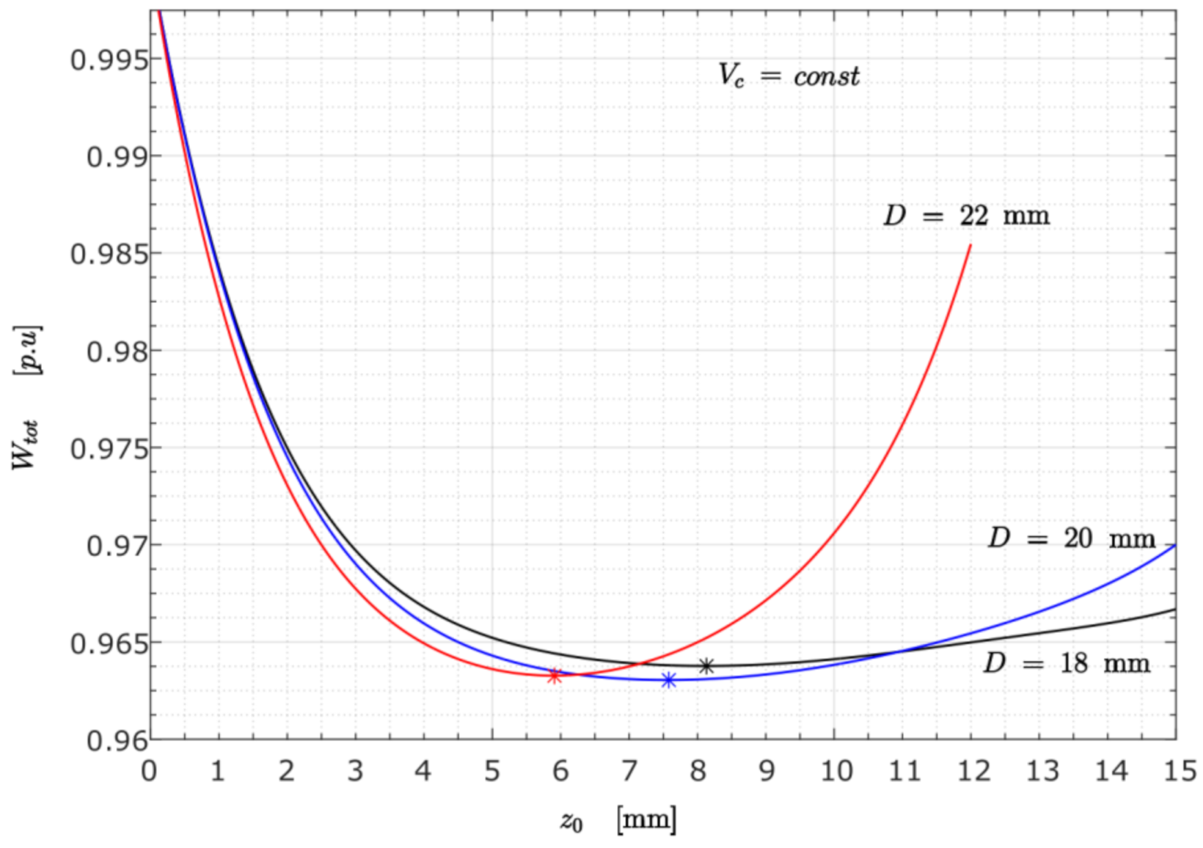
3.3.4. Case D (Variation of the PM’s Diameter at Constant PM Volume)
The results presented in Table 6 and Figure 20 and Figure 21 demonstrate the influence of the PM’s geometry proportions on its equilibrium height . The analysis was performed with three different values of : 9 mm, 10 mm, and 11 mm. The geometry of the PM was conditioned with the assumption of constant PM volume. Other relevant parameters used with the analysis were mm, , T, mm, and mm. The mesh parameters were the same as those stated in Table 1.
3.3.5. Case E (Variation of the Container’s Diameter at Constant Container’s Volume)
The geometry of the container was varied similarly as in the previous case (case D). The container’s diameter () was varied at a constant container volume. The results presented in Table 7 and Figure 22 and Figure 23 show how the container’s proportions impact the PM’s equilibrium height . Other relevant parameters used with the analysis were mm, , T, mm, and mm. The mesh parameters were the same as those stated in Table 1.
4. Conclusions
In the current study, the numerical investigation of the equilibrium height of a PM immersed in MF was carried out in two different concepts: the surface integral method (SIM) and the employment of the energy method (EM). The latter approach brings novelty to the field. To verify the proposed method, a comprehensive parametric analysis was carried out on the subject. The analysis encompassed five cases, where the properties of both MF and the PM were varied. For each of the five cases, the PM’s equilibrium height was calculated with both methods, i.e., SIM and EM. In addition to the numerical results and analysis, the reader is also provided with the essential theoretical background on which the energy concept is based.
The following can be summarized, focusing on the EM, presented as an alternative and novel method to calculate the equilibrium levitation height of a PM drowned in MF. In both concepts based on EM and SIM, magnetic field distributions in space are essential data which are nowadays, almost without exception, obtained numerically, most commonly with FEM. From that point of view, both methods are practically equivalent in the computational time consumption. The main advantage of the EM over the SIM is that the adoption of the Maxwell stress tensor surface integral can be avoided. As mentioned in the Introduction, a numerical problem arises when evaluating this integral on a finite element mesh made of first-order triangles [20].
The following remarks can be stated based on the parametric analysis.
- By increasing the radius of the measuring rod (), the PM’s levitation height will tend to reach a higher level. The reason is evident; while the rod usually consists of non-magnetic material, the fluid-magnetic pressure at the PM’s top face is going to produce a lower force than at the PM’s bottom face. The difference in this pressure acts upward, hence, the magnet will levitate at a higher level. For this case, the error between SIM and EM was less than 1%.
- The magnetic properties of the MF are reflected in the value of relative permeability which is, here, assumed as a constant. Truly speaking, this is only a rough approximation. Namely, in real magnetic fluids, the magnetizing characteristic are non-linear, and the concentration of the particles also decreases with the distance from the magnet. However, even with this simplification, the conclusion can be declared that the PM immersed in a magnetic fluid with lower permeability will experience a weaker magnetic buoyancy force. Consequently, the levitation height will be lower to some extent.
- The same can be derived by considering the problem in the light of the energy. In highly permeable MF, the PM would rather be centered in the fluid, because its magnetostatic energy is minimal there. By decreasing the MF’s permeability the magnetostatic energy increases and its variation with respect to the levitation height becomes smaller, thus, the influence of the gravitational energy comes to the fore, and moves the minimum of the total energy curve towards a lower value. The results’ comparison obtained by the SIM and EM for the case shows that the error between the methods is less than 4%. The results fit better at higher values of the MF’s permeabilities.
- A remanent magnetic flux density is a property of a PM, and from the presented results, it is evident that higher leads to a higher levitation height. The remanence is related to the origin of the magnetic force in the MF, and, therefore, it is reasonable to expect such an effect. Again, a good agreement was achieved between the methods. The maximum error value was about 5%.
- Variation in the PM’s geometry shows that the levitation height is proportional to the PM’s diameter defining the top and the bottom surface area. The theoretical explanation is straightforward. The magnetic levitation force appears mainly as a consequence of a fluid-magnetic pressure acting on those surfaces. An increase in the surface area will result in a rise in the magnetic levitation force. The numerical results attained by the SIM and EM showed the same tendency, with the maximum error of 12.2%.
- Change in the container’s geometry acts oppositely to the change in the PM’s geometry as discussed previously. Namely, in this case, the magnetic force acting on the PM reduces proportionally to the ratio of the diameters of the PM and container. The error in the analysis between the methods was less than 1%.
Regarding the presented numerical results, both methods, the SIM and EM, predicted similar results. The maximum deviation between the results obtained by the methods was 12.2%, but for most of the cases, the expected error should not exceed a few percent. However, the SIM for Case A was verified experimentally, where the maximum error in the lower half of the container appeared to be 15% [15]. The authors of the text believe that the error can be reduced significantly by an improved MF model that apprehends the magnetic nonlinearity and inhomogeneity of the particle distribution. The researchers in the field may find this a topic to focus on.
In the end, a final remark on the subject can be made as follows: when the numerical evaluation of the PM levitation height is in question, satisfactory results can be attained by the proposed EM approach.
Author Contributions
Conceptualization, A.H., M.J., M.T. (Mladen Trlep) and M.T (Mislav Trbusic); methodology, M.T. (Mislav Trbusic); software, M.T. (Mislav Trbusic); validation, M.T. (Mislav Trbusic); formal analysis, M.T. (Mislav Trbusic); investigation, M.T. (Mislav Trbusic); resources, M.T. (Mladen Trlep); data curation, M.J.; writing—original draft preparation, M.T. (Mislav Trbusic); writing—review and editing, M.T. (Mislav Trbusic), M.J., M.T. (Mladen Trlep) and A.H.; visualization, M.T. (Mislav Trbusic); supervision, A.H.; project administration, M.T. (Mladen Trlep); funding acquisition, M.T. (Mladen Trlep). All authors have read and agreed to the published version of the manuscript.
Funding
This work was supported by the Slovenian Research Agency under Grant P2-0114.
Institutional Review Board Statement
Not applicable.
Informed Consent Statement
Not applicable.
Data Availability Statement
All data are presented in the article.
Conflicts of Interest
The authors declare no conflict of interest.
References
- Rosensweig, R.E. Fluidmagnetic Buoyancy. AIAA J. 1966, 4, 1751–1758. [Google Scholar] [CrossRef]
- Rosensweig, R.E. Buoyancy and Stable Levitation of a Magnetic Body immersed in a Magnetizable Fluid. Nature 1966, 210, 613–614. [Google Scholar] [CrossRef]
- Moskowitz, R.; Stahl, P.; Reed, W.R. Inertia Damper Using Ferrofluid. US Patent 4123675, 31 October 1978. [Google Scholar]
- Miller, D.L. Magnetic Viscous Damper. US Patent 4200003, 29 April 1980. [Google Scholar]
- Kogure, T. Damper Device for a Motor. US Patent 5191811, 9 March 1993. [Google Scholar]
- Bashtovoi, V.G.; Kabachikov, D.N.; Kolobov, A.Y.; Samoylov, V.B.; Vikoulenkov, A.V. Research of the dynamics of a magnetic fluid dynamic absorber. J. Magn. Magn. Mater. 2002, 252, 312–314. [Google Scholar] [CrossRef]
- Wang, Z.; Bossis, G.; Volkova, O.; Bashtovoi, V.; Krakov, M.S. Active Control of Rod Using Magnetic Fluids. J. Intell. Mater. Syst. Struct. 2003, 14, 93–97. [Google Scholar] [CrossRef]
- Yang, W. Magnetic levitation force exerted on the cylindrical magnet in a ferrofluid damper. J. Vib. Control 2015, 23, 2345–2354. [Google Scholar] [CrossRef]
- Yao, J.; Chang, J.; Li, D.; Yang, X. The dynamics analysis of a ferrofluid shock absorber. J. Magn. Magn. Mater. 2016, 402, 28–33. [Google Scholar] [CrossRef]
- Piso, M.I. Applications of magnetic fluids for inertial sensors. J. Magn. Magn. Mater. 1999, 201, 380–384. [Google Scholar] [CrossRef]
- Qian, L.; Li, D.; Yu, J. Study of the Second-Order Levitation Force in the Magnetic Fluid Accelerometer. IEEE Sens. J. 2015, 15, 6805–6810. [Google Scholar] [CrossRef]
- Yu, J.; He, X.; Li, D.; Li, W. Effective and Practical Methods to Calculate the Second-Order Buoyancy in Magnetic Fluid Acceleration Sensor. IEEE Sens. J. 2018, 18, 2278–2284. [Google Scholar] [CrossRef]
- Yang, W.; Li, D.; He, X.; Li, Q. Calculation of magnetic levitation force exerted on the cylindrical magnets immersed in ferrofluid. Int. J. Appl. Electromagn. Mech. 2012, 40, 37–49. [Google Scholar] [CrossRef]
- Yang, W.; Wang, P.; Hao, R.; Ma, B. Experimental verification of radial magnetic levitation force on the cylindrical magnets in ferrofluid dampers. J. Magn. Magn. Mater. 2017, 426, 334–339. [Google Scholar] [CrossRef]
- Yu, J.; Chen, J.; Li, D. Experimental error analysis of measuring the magnetic self-levitation force experienced by a permanent magnet suspended in magnetic fluid with a nonmagnetic rod. J. Magn. Magn. Mater. 2019, 469, 323–328. [Google Scholar] [CrossRef]
- Yu, J.; Chen, D.; Cai, Z.; Li, D.; Cao, Q.; Qian, L. Research on the magnetic fluid levitation force received by a permanent magnet suspended in magnetic fluid: Consideration a surface instability. J. Magn. Magn. Mater. 2019, 492, 165678. [Google Scholar] [CrossRef]
- Sudo, S.; Takaki, Y.; Hashiguchi, Y.; Nishiyama, H. Magnetic Fluid Devices for Driving Micro Machines. JSME Int. J. 2005, 48, 464–470. [Google Scholar] [CrossRef] [Green Version]
- Imai, S.; Tsukioka, T. A magnetic MEMS actuator using a permanent magnet and magnetic fluid enclosed in a cavity sandwiched by polymer diaphragms. Precis. Eng. 2014, 38, 548–554. [Google Scholar] [CrossRef]
- Yu, J.; He, X.; Li, D.; Li, W. Boundary interface condition of magnetic fluid determines the magnetic levitation force experienced by a permanent magnet suspended in the magnetic fluid. Phys. Fluids 2018, 30, 092004. [Google Scholar] [CrossRef]
- Meeker, D. Finite Element Method Magnetics—User’s Manual. Verison 4.2. 2007, pp. 44–46. Available online: https://www.femm.info/Archives/doc/manual42.pdf (accessed on 31 August 2021).
- Bastos, J.P.A.; Sadowski, N. Electromagnetic Modeling by Finite Element Methods, 1st ed.; Marcel Dekker Inc.: New York, NY, USA, 2003; pp. 381–383. [Google Scholar]
- Rosensweig, R.E. Ferrohydrodynamics, 1st ed.; Dover Publications, Inc.: New York, NY, USA, 2014. [Google Scholar]
- Trbušić, M.; Beković, M.; Trlep, M.; Hamler, A. Nonlinear analysis of magnetic liquid free surface deformation in a 3D space. J. Magn. Magn. Mater. 2019, 482, 364–369. [Google Scholar] [CrossRef]
Figure 1.
The basic deployment of the problem.

Figure 2.
Permanent magnet immersed in magnetic fluid. Dashed lines indicate the integration paths over the container’s inner surface and PM surfaces , respectively.
Figure 2.
Permanent magnet immersed in magnetic fluid. Dashed lines indicate the integration paths over the container’s inner surface and PM surfaces , respectively.

Figure 3.
Visual representation of how magnetic fluid pressure contributes to the self-levitation mechanism: (a) In this position, a magnetic field is much higher at the bottom of the container than it is at the top of it, thus, the magnetic fluid pressure is also higher at the bottom, which results in PM upward movement; (b) In the stable levitation position, or in equilibrium height, the magnetic fluid pressure is balanced within the container; (c) If the PM tends to move up somehow, the pressure on the top increases due to the higher magnetic field, and the PM starts to move toward the stable position.

Figure 4.
Magnetic levitation force calculated through the integration over the container surface: (a,b) The integration path is not affected by the object’s non-intersecting the surface over which it is integrated; (c) The integration path involving materials with different magnetic properties.
Figure 4.
Magnetic levitation force calculated through the integration over the container surface: (a,b) The integration path is not affected by the object’s non-intersecting the surface over which it is integrated; (c) The integration path involving materials with different magnetic properties.

Figure 5.
Schematic representation of a magnetic field caused by the PM levitating in the MF.
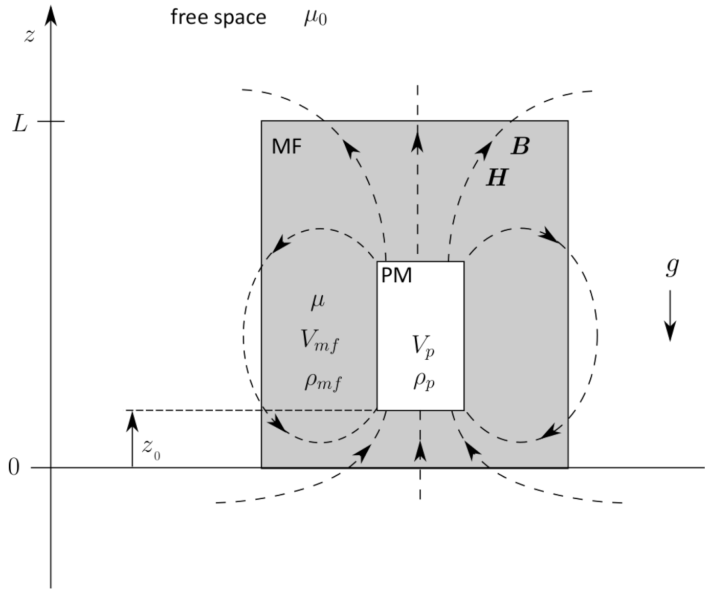
Figure 6.
Simplified analytical model: (a) The MF is extended to infinity with respect to the x and y directions, and the PM is presented as an unbounded infinitesimal thin layer; (b) Magnetic field intensity decreases exponentially with the distance from the magnet, and has discontinuity when facing material with different permeability; (c) Magnetic flux density decreases exponentially and continuously with the distance from the magnet.
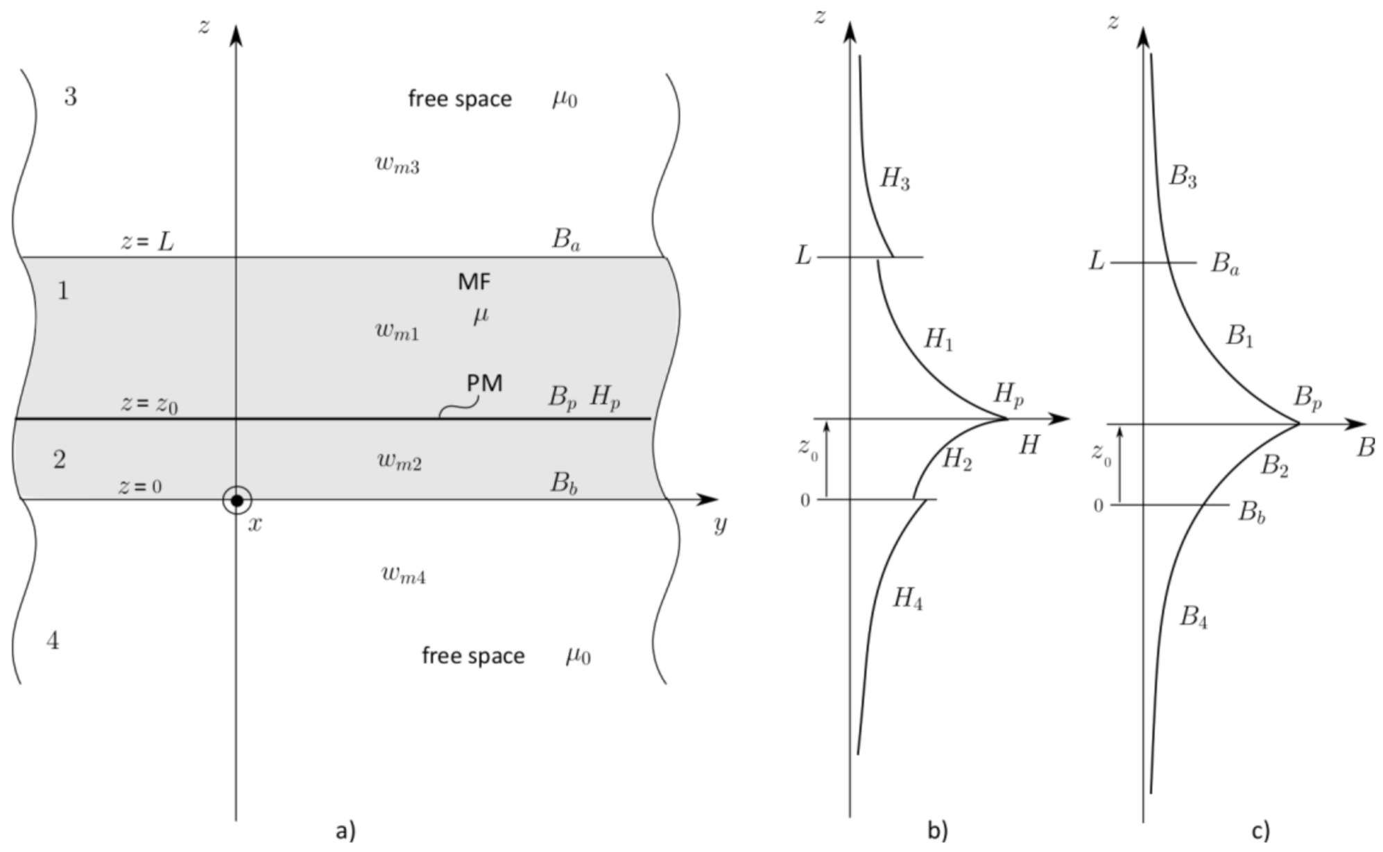
Figure 7.
A column of the simplified analytical model is considered in a qualitative analysis of a stable levitation height.
Figure 7.
A column of the simplified analytical model is considered in a qualitative analysis of a stable levitation height.

Figure 8.
Results of a qualitative analysis based on the energy method. A stable levitation height is attained at the minimum of the total energy. The influence of the levitating object’s weight acts in the way to move the equilibrium height towards the lower value. Data used in the analysis are given as follows T, mm, mm2, mm, m−1, , mm, and mm. Each of the curves are normalized by the maximum value of the total energy.

Figure 9.
(a) Dimensions of the model; (b) FEMM 2D axisymmetric model in preprocessor mode, where mesh details are shown. Denser mesh is prescribed to the integration paths used with the SIM.
Figure 9.
(a) Dimensions of the model; (b) FEMM 2D axisymmetric model in preprocessor mode, where mesh details are shown. Denser mesh is prescribed to the integration paths used with the SIM.

Figure 10.
Calculated and measured values of the second order buoyancy force and determination of the equilibrium state at the intersection point between and . The intersection is established with respect to the calculated values, and its value is mm. Measured data were acquired from [15] (p. 327—Figure 5b) for the case where the diameter of the rod is 2 mm.
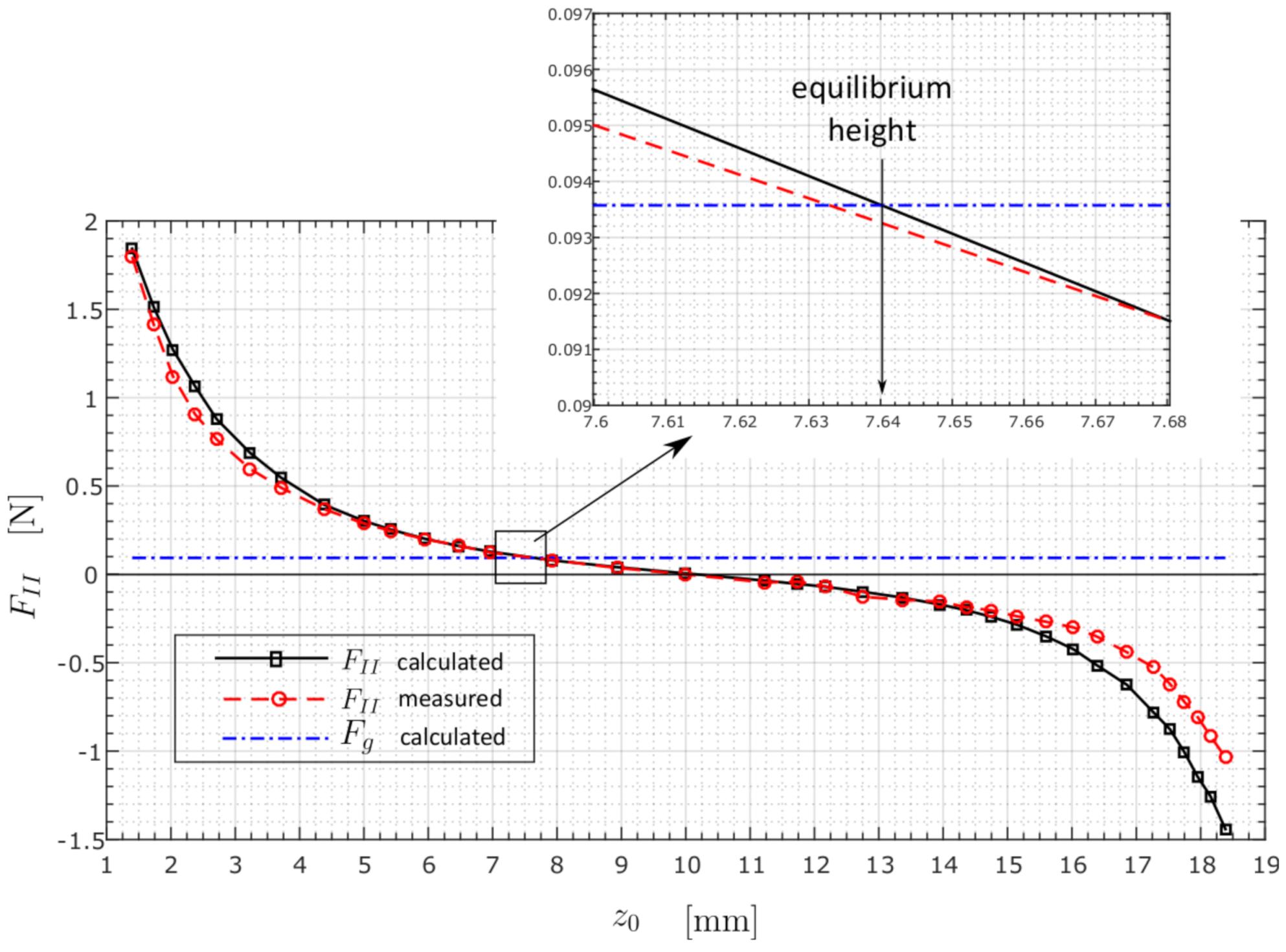
Figure 11.
Results obtained by the energy method, where the equilibrium height appears at a minimum of total energy with the value of mm.
Figure 11.
Results obtained by the energy method, where the equilibrium height appears at a minimum of total energy with the value of mm.
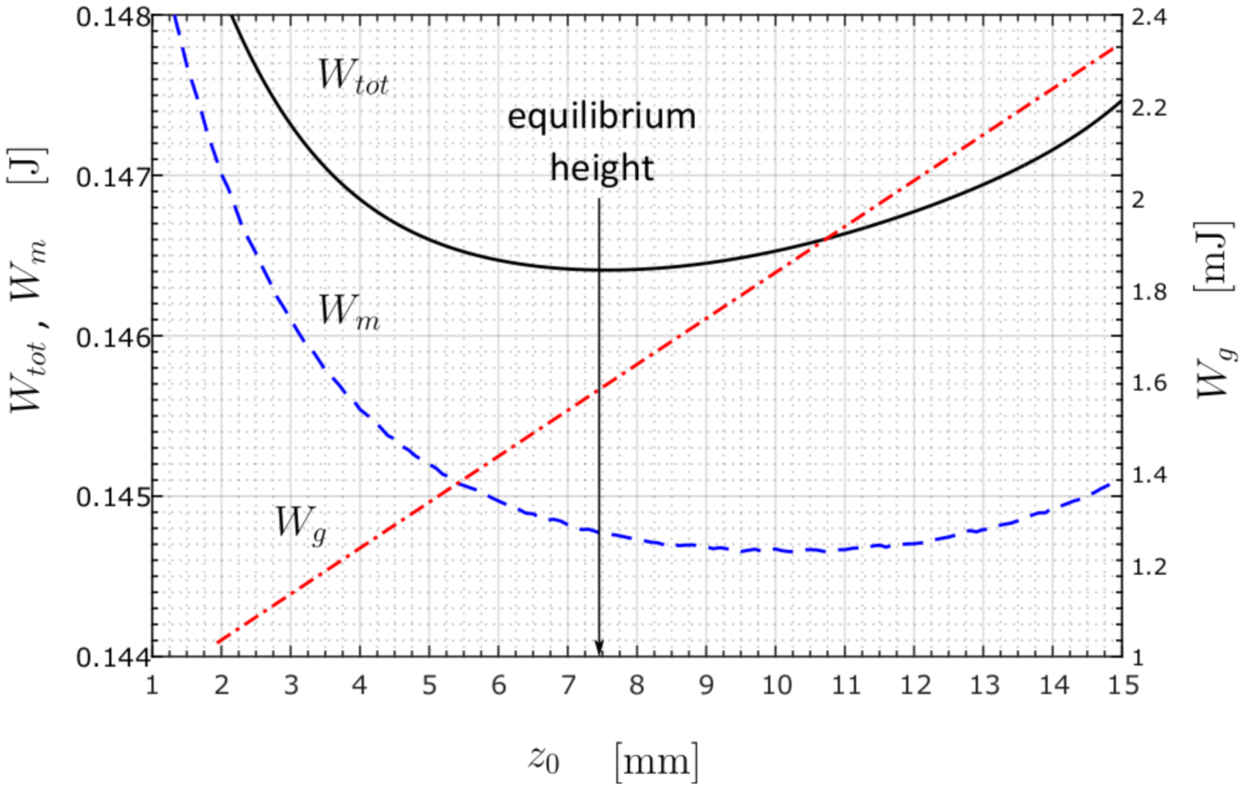
Figure 12.
The measured and calculated curves of magnetic levitation force for the case mm. The force was calculated by the SIM. An intersection between the gravitational and mag-netic levitation force is shown in the magnified window. Measured data were acquired from ref. [15].
Figure 12.
The measured and calculated curves of magnetic levitation force for the case mm. The force was calculated by the SIM. An intersection between the gravitational and mag-netic levitation force is shown in the magnified window. Measured data were acquired from ref. [15].

Figure 13.
The measured and calculated curves of magnetic levitation force for the case mm. The force was calculated by the SIM. An intersection between the gravitational and mag-netic levitation force is shown in the magnified window. Measured data were acquired from ref. [15].
Figure 13.
The measured and calculated curves of magnetic levitation force for the case mm. The force was calculated by the SIM. An intersection between the gravitational and mag-netic levitation force is shown in the magnified window. Measured data were acquired from ref. [15].

Figure 14.
The measured and calculated curves of magnetic levitation force for the case mm. The force was calculated by the SIM. An intersection between the gravitational and mag-netic levitation force is shown in the magnified window. Measured data were acquired from ref. [15].
Figure 14.
The measured and calculated curves of magnetic levitation force for the case mm. The force was calculated by the SIM. An intersection between the gravitational and mag-netic levitation force is shown in the magnified window. Measured data were acquired from ref. [15].
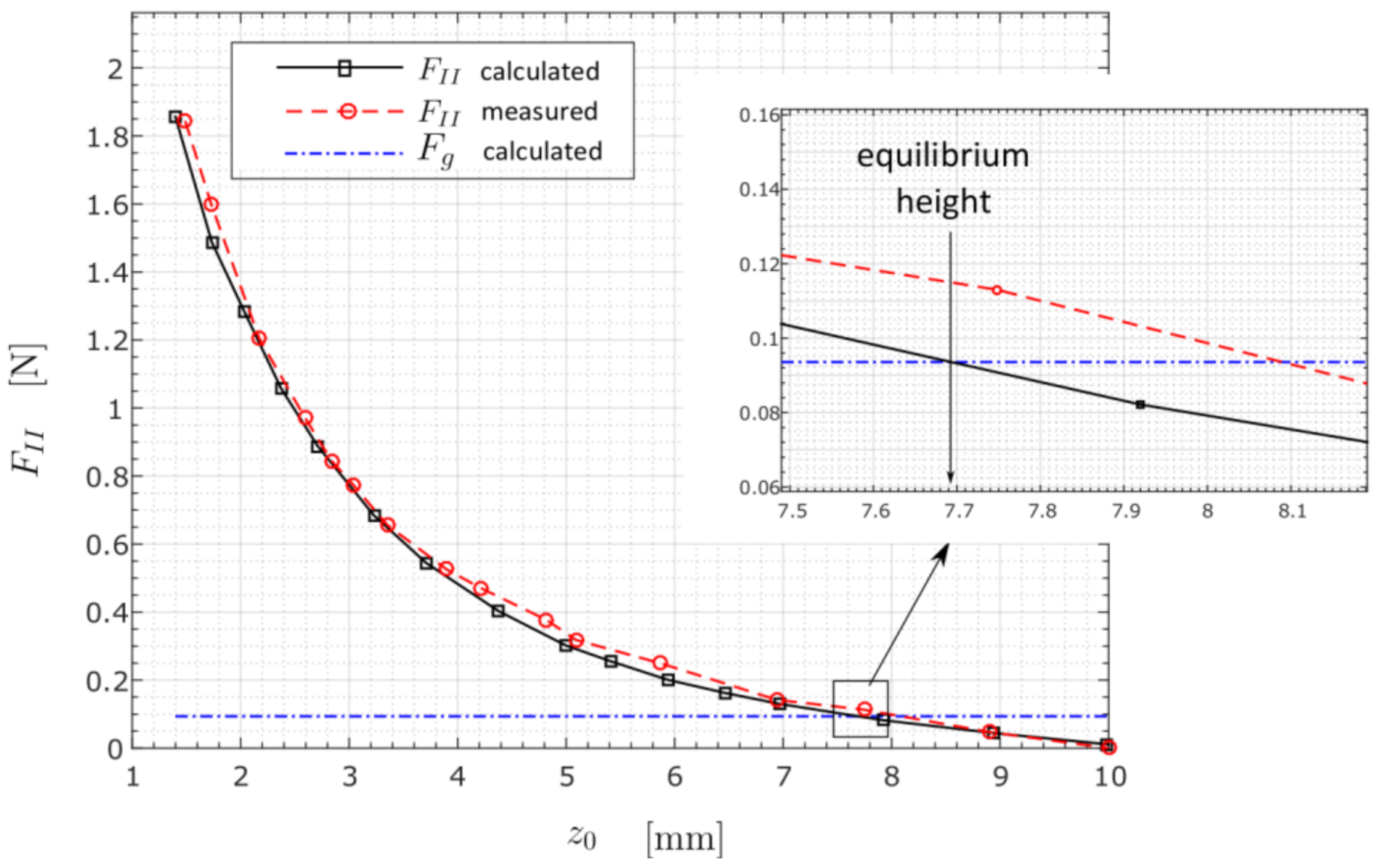
Figure 15.
The PM’s equilibrium height calculated by EM. The results are shown for three different values of the rod’s radius, i.e., mm, mm and mm, respectively. The minimum value on the individual curve is indicated with the Asterisk (*). Each of the curves was nor-malized by its maximum value.
Figure 15.
The PM’s equilibrium height calculated by EM. The results are shown for three different values of the rod’s radius, i.e., mm, mm and mm, respectively. The minimum value on the individual curve is indicated with the Asterisk (*). Each of the curves was nor-malized by its maximum value.

Figure 16.
The calculated curves of magnetic levitation force for three different values of MF’s permeability, i.e., , , and , respectively. The force was calculated by the SIM. The stable levitation height appears where the individual curve intersects the gravitational force line .
Figure 16.
The calculated curves of magnetic levitation force for three different values of MF’s permeability, i.e., , , and , respectively. The force was calculated by the SIM. The stable levitation height appears where the individual curve intersects the gravitational force line .
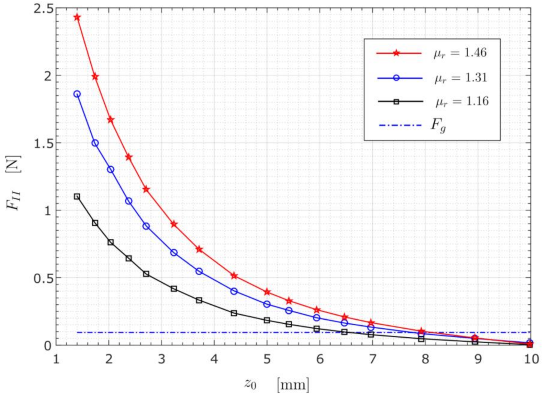
Figure 17.
The PM’s equilibrium height calculated by EM. The results are given for three different values of the MF’s permeability, i.e., , , and , respectively. The mini-mum value on the individual curve is indicated with the Asterisk (*). Each of the curves was normalized by its maximum value.
Figure 17.
The PM’s equilibrium height calculated by EM. The results are given for three different values of the MF’s permeability, i.e., , , and , respectively. The mini-mum value on the individual curve is indicated with the Asterisk (*). Each of the curves was normalized by its maximum value.

Figure 18.
The calculated curves of magnetic levitation force for three different values of the PM’s remanence, i.e., T, T, and T, respectively. The force was calculated by the SIM. The stable levitation height appears where the individual curve in-tersects the gravitational force line .
Figure 18.
The calculated curves of magnetic levitation force for three different values of the PM’s remanence, i.e., T, T, and T, respectively. The force was calculated by the SIM. The stable levitation height appears where the individual curve in-tersects the gravitational force line .

Figure 19.
The PM’s equilibrium height calculated by EM. The results are shown for three different values of the PM’s remanence, i.e., T, T, and T, respectively. The minimum value on the individual curve is indicated with the Asterisk (*). Each of the curves were normalized by its maximum value.
Figure 19.
The PM’s equilibrium height calculated by EM. The results are shown for three different values of the PM’s remanence, i.e., T, T, and T, respectively. The minimum value on the individual curve is indicated with the Asterisk (*). Each of the curves were normalized by its maximum value.
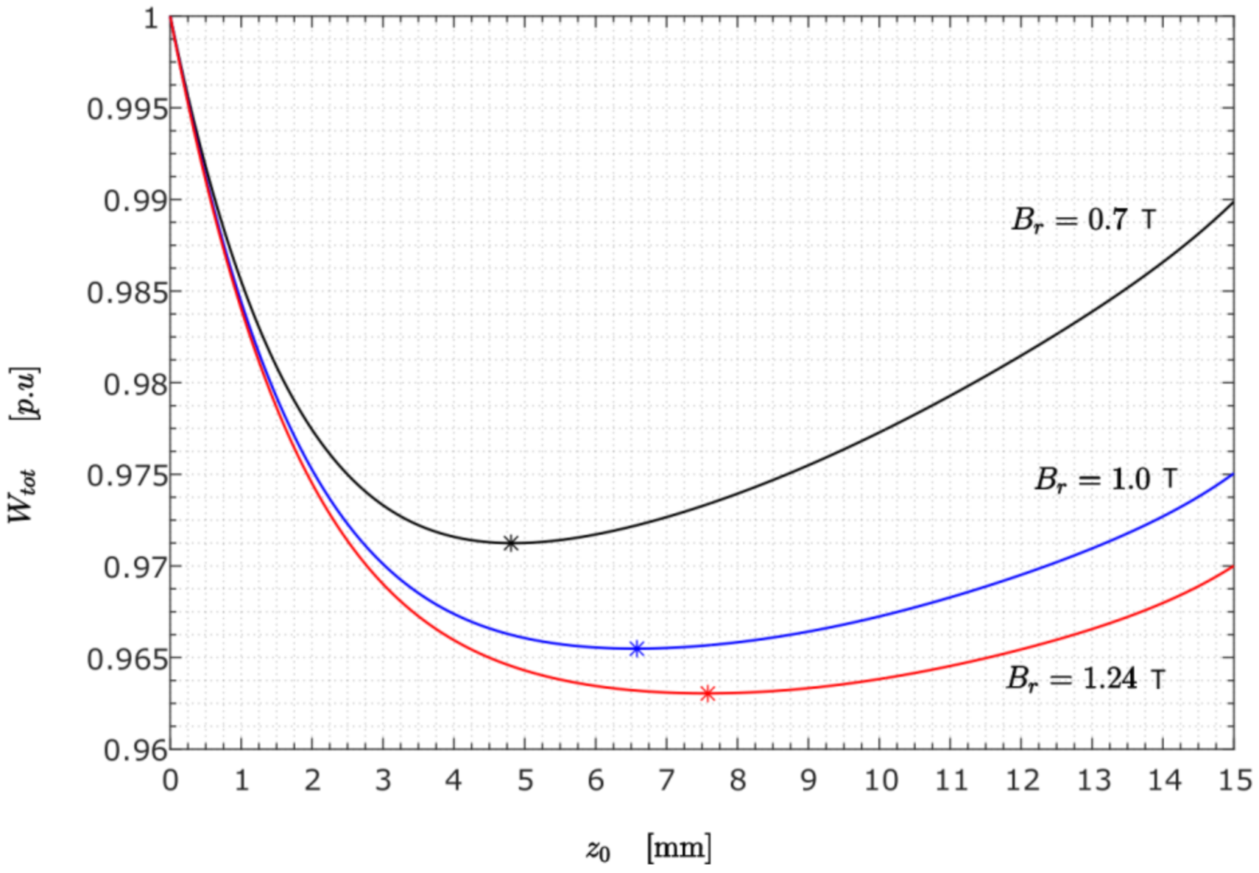
Figure 20.
The calculated curves of magnetic levitation force for three different values of the PM’s diameter, i.e., mm, mm, and mm, respectively. The force was calculated by the SIM. The stable levitation height appears where the individual curve in-tersects the gravitational force line . In calculations, the PM’s volume remained unchanged.

Figure 21.
The PM’s equilibrium height calculated by EM. The results are shown for three different values of the PM’s diameter, i.e., mm, mm, and mm, respectively. The minimum value on the individual curve is indicated with the Asterisk (*). Each of the curves was normalized by its maximum value. In the calculations, the PM’s volume remained un-changed.
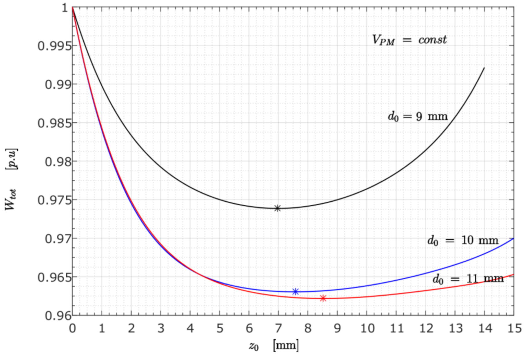
Figure 22.
The calculated curves of magnetic levitation force for three different values of container diameter, i.e., mm, mm, and mm, respectively. The force was calculated by the SIM. The stable levitation height appears where the individual curve in-tersects the gravitational force line . In the calculations the container’s volume re-mained unchanged.
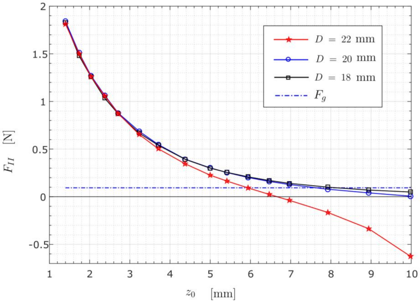
Figure 23.
The PM’s equilibrium height calculated by EM. The results are shown for three different values of the container’s diameter, i.e., mm, mm, and mm, respectively. The minimum value on the individual curve is indicated with the Asterisk (*). Each of the curves was normalized by its maximum value. In calculations the container’s volume remained unchanged.

Table 1.
Values of the parameters used with the model 1.
| Permanent Magnet (PM) | Magnetic Fluid (MF) | Rod | Free Space | |
|---|---|---|---|---|
| material | NdFeB (N38) | - | copper | Air |
| 𝜌 [kgm−3] | 7450 | 1377.6 | 8900 | 1.2 |
| 1 | 1.31 | 1 | 1 | |
| [T] | 1.24 | - | - | - |
| [kAm−1] | 986.7 | - | - | - |
| 0 | 0.31 | 0 | 0 | |
| Max. mesh size in material [mm] | 0.25 | 0.25 | 0.5 | 10 |
| Max. mesh size at boundary [mm] | 0.05 | 0.05 | - | - |
1 The values are selected to fit well with the ones in ref. [15].
Table 2.
Numerical values pertain to calculated and measured values of magnetic levitation force. The error analysis is given for the difference between the calculated and measured quantities.
Table 2.
Numerical values pertain to calculated and measured values of magnetic levitation force. The error analysis is given for the difference between the calculated and measured quantities.
| Levitation Height 1 | Magnetic Levitation Force—Calculated | Magnetic Levitation Force—Measured 1 | Error |
|---|---|---|---|
| 1.40 | 1.84 | 1.80 | 2.2 |
| 1.73 | 1.51 | 1.41 | 6.6 |
| 2.03 | 1.27 | 1.12 | 11.8 |
| 2.37 | 1.07 | 0.91 | 15.0 |
| 2.71 | 0.88 | 0.76 | 13.6 |
| 3.23 | 0.69 | 0.60 | 13.0 |
| 3.71 | 0.55 | 0.49 | 10.9 |
| 4.38 | 0.39 | 0.37 | 5.1 |
| 5.00 | 0.30 | 0.29 | 3.3 |
| 5.41 | 0.25 | 0.25 | 0.0 |
| 5.94 | 0.20 | 0.20 | 0.0 |
| 6.47 | 0.16 | 0.16 | 0.0 |
| 6.97 | 0.13 | 0.12 | 7.7000 |
| 7.92 | 0.08 | 0.08 | 0.0 |
| 8.94 | 0.04 | 0.04 | 0.0 |
| 9.98 | 0.01 | 0.00 | - |
| 11.23 | −0.04 | −0.05 | −25.0 |
| 11.74 | −0.05 | −0.04 | 20.0 |
| 12.16 | −0.07 | −0.07 | 0.00 |
| 12.76 | −0.10 | −0.13 | −30.0 |
| 13.37 | −0.13 | −0.14 | −7.7 |
| 13.95 | −0.17 | −0.15 | 11.8 |
| 14.35 | −0.20 | −0.19 | 5.0 |
| 14.75 | −0.24 | −0.20 | 16.7 |
| 15.15 | −0.29 | −0.24 | 17.2 |
| 15.60 | −0.35 | −0.27 | 22.9 |
| 16.02 | −0.42 | −0.30 | 28.6 |
| 16.39 | −0.51 | −0.35 | 31.4 |
| 16.85 | −0.62 | −0.44 | 29.0 |
| 17.27 | −0.78 | −0.53 | 32.1 |
| 17.53 | −0.88 | −0.62 | 29.5 |
| 17.75 | −1.01 | −0.72 | 28.7 |
| 17.95 | −1.14 | −0.81 | 28.9 |
| 18.15 | −1.26 | −0.92 | 27.0 |
| 18.39 | −1.44 | −1.04 | 27.8 |
1 Data were acquired from ref. [15] (p. 327—Figure 5b) for the case where the diameter of the rod is 2 mm.
Table 3.
The impact of the rod’s radius on the PM’s equilibrium height.
| Method | |||
|---|---|---|---|
| SIM | 7.59 | 7.64 | 7.69 |
| EM | 7.53 | 7.58 | 7.63 |
| Experiment 1 | 8.20 | 7.63 | 8.09 |
| Error ∆𝜖 | 0.8% | 0.8% | 0.8% |
1 Data were acquired from ref. [15].
Table 4.
The impact of the MF’s relative permeability on the PM’s equilibrium height.
| Method | |||
|---|---|---|---|
| SIM | 6.56 | 7.64 | 8.13 |
| EM | 6.32 | 7.58 | 8.08 |
| Error | 3.6% | 0.8% | 0.6% |
Table 5.
The influence of the MF’s remanence flux density on the PM’s equilibrium height.
| Method | |||
|---|---|---|---|
| SIM | 5.08 | 6.73 | 7.64 |
| EM | 4.82 | 6.57 | 7.58 |
| [%] | 5.1% | 2.4% | 0.8% |
Table 6.
The impact of the PM’s geometry proportion on its equilibrium height.
| Method | |||
|---|---|---|---|
| SIM | 6.22 | 7.64 | 8.66 |
| EM | 6.98 | 7.58 | 8.53 |
| [%] | −12.2% | 0.8% | 1.5% |
Table 7.
The impact of the container’s geometry proportion on the PM’s equilibrium height.
| Method | |||
|---|---|---|---|
| SIM | 8.15 | 7.64 | 5.93 |
| EM | 8.13 | 7.58 | 5.90 |
| [%] | 0.2% | 0.8% | 0.5% |
Publisher’s Note: MDPI stays neutral with regard to jurisdictional claims in published maps and institutional affiliations. |
© 2021 by the authors. Licensee MDPI, Basel, Switzerland. This article is an open access article distributed under the terms and conditions of the Creative Commons Attribution (CC BY) license (https://creativecommons.org/licenses/by/4.0/).
Share and Cite
MDPI and ACS Style
Trbušić, M.; Jesenik, M.; Trlep, M.; Hamler, A. Energy Based Calculation of the Second-Order Levitation in Magnetic Fluid. Mathematics 2021, 9, 2507. https://doi.org/10.3390/math9192507
AMA Style
Trbušić M, Jesenik M, Trlep M, Hamler A. Energy Based Calculation of the Second-Order Levitation in Magnetic Fluid. Mathematics. 2021; 9(19):2507. https://doi.org/10.3390/math9192507
Chicago/Turabian StyleTrbušić, Mislav, Marko Jesenik, Mladen Trlep, and Anton Hamler. 2021. "Energy Based Calculation of the Second-Order Levitation in Magnetic Fluid" Mathematics 9, no. 19: 2507. https://doi.org/10.3390/math9192507
Note that from the first issue of 2016, this journal uses article numbers instead of page numbers. See further details here.