Bayesian Variable Selection with Applications in Health Sciences

Abstract

In health sciences, identifying the leading causes that govern the behaviour of a response variable is a question of crucial interest. Formally, this can be formulated as a variable selection problem. In this paper, we introduce the basic concepts of the Bayesian approach for variable selection based on model choice, emphasizing the model space prior adoption and the algorithms for sampling from the model space and for posterior probabilities approximation; and show its application to two common problems in health sciences. The first concerns a problem in the field of genetics while the second is a longitudinal study in cardiology. In the context of these applications, considerations about control for multiplicity via the prior distribution over the model space, linear models in which the number of covariates exceed the sample size, variable selection with censored data, and computational aspects are discussed. The applications presented here also have an intrinsic statistical interest as the proposed models go beyond the standard general linear model. We believe this work will broaden the access of practitioners to Bayesian methods for variable selection.

1. Introduction

In applied sciences, identifying the leading causes that govern a response variable is a question of crucial interest. In a cardiology study, for example, we could be interested in knowing which aspects of the clinical history influence the time until the occurrence of a major adverse event.

Although this problem could be approached from a purely theoretical perspective by building a mathematical model accurately describing the physics underlying the phenomenon under study (see, e.g., [1] for a model on the cardiac physiology) the more popular and pragmatic perspective to address it is using statistical methodology. In this framework, an experimental study is conducted where the response variable (Y) is measured in a sample of individuals, together with a large number of possible explanatory variables or covariates ($X_1,X_2,\dots ,X_p$). A probabilistic model is then used not only to describe the relationship between Y and $X_1,X_2,\dots ,X_p$ but also to explicitly acknowledge the effect—of a random nature—of imprecisions in the measurements and of variables not considered in the study. From this starting point, the question reduces to decide which of the covariates have a relevant impact on the response, a problem known as variable selection.

Because of its relevance, variable selection has been during decades, and still is, a leading topic of research with contributions from many areas of statistics. A useful and didactic classification of methods for variable selection distincts between ‘estimation’ and ‘model choice’ based strategies (for a similar argument see e.g., [2,3]). The first proceeds based on inferences obtained from the model containing all covariates (the full model) meanwhile the second assumes that every possible combination of covariates provides an autonomous description of the phenomenon. Model choice approach to variable selection is based on the evaluation of the endorsement that each single model receives from the data. As an illustration and to make the distinction clearer, a regularization method (like lasso) falls in the first category while a stepwise procedure belongs to the second.

Both the frequentist and the Bayesian schools—the two main statistical paradigms—have been used to construct estimation and model choice methods. Nonetheless, the Bayesian approach better accommodates the idiosyncrasy of the second approach since it naturally handles the different sources of uncertainty: it is unknown which is the true model and which is the true value of the parameters within each model. Finally, the available information is processed through the Bayes theorem, providing the posterior distribution which assigns the updated probability of every potential model, in light of the data. Among the advantages, the resulting approach is automatically parsimonious (promoting simpler over complex models for a comparable fit) and provides the right control for multiplicity (a large number of models is fit and it is quite likely that just by chance a ‘good’ spurious model appears). Additionally, the results are arguably very rich allowing to provide uncertainty measures concerning the selection exercise as well as model averaging inferences and predictions considering all sources of uncertainties in the problem. For a careful description of the advantages of the Bayesian method for model choice, the reader is referred to [4].

In this paper, we introduce the basic concepts of the Bayesian approach for variable selection based on model choice. In particular, Section 2 presents the main ingredients and discusses the principal challenges in the implementation of the method. Our main contribution is the application of this methodology to two real problems in health sciences, described in Section 3 and Section 4. The aim here is twofold: on the one hand, to illustrate the potential of this approach for health researchers; on the other hand, to highlight some of the difficulties that appear in the Bayesian method and that will be the base of future theoretical developments. Section 3 deals with model selection in linear regression with thousands of potential covariates, in the field of genetics. The issue of variable selection with censored data is addressed in Section 4, for the analysis of a study of events post-treatment in cardiology. To finish, Section 5 is devoted to discussion.

2. Variable Selection Based on Bayesian Model Choice

Let y be the n-size vector that contains the observed data for Y. Independently on the distribution assumed for Y and its relation with the independent variables, the collection of models that arise when the different combinations of covariates is listed can be compactly expressed using a binary parameter vector $\mathit{\gamma }=({\gamma }_1,\dots ,{\gamma }_p)$. Here ${\gamma }_i=1$ if the response depends on $X_i$ and zero otherwise. For example, the model including only $X_2$ corresponds to $\mathit{\gamma }=(0,1,0,\dots ,0)$. We label each of these models $M_{\gamma }$ or simply $\mathit{\gamma }$. The set containing all potential models is called the model space and its cardinality is $2^p$. With an abuse of notation, the simplest model $M_0$ is traditionally named the ‘null’ model and the model containing all covariates, $M_1$, is the ‘full’ model.

Let $f_{\gamma }(\mathit{y}\mid {\mathit{\theta }}_{\gamma })$ be the probability density function of y given the vector parameter ${\mathit{\theta }}_{\gamma }$, which expresses the relation between the dependent variable and the active covariates in $\mathit{\gamma }$. In normal linear models, $f_{\gamma }$ would be a multivariate normal with mean a linear combination of the active variables and certain unknown variance. The parameter vector ${\mathit{\theta }}_{\gamma }$ in that case contains the regression coefficients (of dimension $k_{\gamma }=\sum {\gamma }_i$) which are specific to that model, $M_{\gamma }$, plus the intercept and the variance of the error which appear in all models.

The posterior distribution of $\mathit{\gamma }$ is the updated probability that each model is the true model given the observed data and can be obtained as:

$$p(M_{{\gamma }^{\prime }}\mid \mathit{y})=\frac{m_{{\gamma }^{\prime }}(\mathit{y})p(M_{{\gamma }^{\prime }})}{{\sum }_{\gamma }{m}_{\gamma }(\mathit{y})p(M_{\gamma })},$$

(1)

where the sum in the denominator ranges in the model space; $p(M_{\gamma })$ is the prior probability of $\gamma$ and $m_{\gamma }(\mathit{y})$ is the corresponding prior predictive marginal:

$$m_{\gamma }(\mathit{y})=\int f_{\gamma }(\mathit{y}\mid {\mathit{\theta }}_{\gamma }){\pi }_{\gamma }({\mathit{\theta }}_{\gamma })d{\mathit{\theta }}_{\gamma }.$$

(2)

In the above equation, ${\pi }_{\gamma }({\mathit{\theta }}_{\gamma })$ is the prior distribution for the model parameters in $M_{\gamma }$.

An equivalent expression for (1) can be derived using Bayes factors [5,6]. A Bayes factor is a relative measure of the evidence contained in the data in favour of a model $M_{\gamma }$ and against another one, $M_{{\gamma }^{\prime }}$. Its mathematical expression corresponds to the ratio of prior predictive marginals between the models. If in (1) we divide numerator and denominator by the marginal of a fixed model ($M_0$, without loss of generality) we obtain:

$$p(M_{{\gamma }^{\prime }}\mid \mathit{y})=\frac{B_{{\gamma }^{\prime }}(\mathit{y})p(M_{{\gamma }^{\prime }})}{{\sum }_{\gamma }{B}_{\gamma }(\mathit{y})p(M_{\gamma })},$$

(3)

where now $B_{\gamma }(\mathit{y})$ are the Bayes factors of $M_{\gamma }$ to $M_0$, that is, $B_{\gamma }(\mathit{y})=m_{\gamma }(\mathit{y})/m_0(\mathit{y})$.

The posterior distribution is a vast piece of information for the variable selection problem. Nevertheless, it needs to be properly summarized in order to provide understandable and useful reports (like with any other posterior distribution). This is a crucial differential aspect of the model choice approach: instead of just selecting a single model (in many cases without any accompanying measure of the error in that choice), the posterior distribution offers an enormous variety of possibilities to gain knowledge about the primary question of measuring the impact that the different covariates have in the response. In many occasions, the summaries reported will be guided by the final interest of researchers, though there are summaries that are quite standard and that we briefly introduce here. One straightforward possibility is to report the model endorsed by the highest probability (known as HPM) jointly with its posterior probability. Alternatively, a list with the first (usually 10 or 20) most likely models and their posterior probabilities is reported, in order to provide an overall idea of the degree of uncertainty clarified by the data. Posterior probabilities lose interest (and interpretability) if they are very small, a situation that arise when p is moderate to large. Another option is to report how many times each model in the list is less probable than the HPM, which conveys how confident we should be in the HPM as a single response to the variable selection problem.

Very popular summaries of $p(M_{{\gamma }^{\prime }}\mid \mathit{y})$ are the posterior inclusion probabilities of the individual variable, that is, the sum of the posterior probabilities of the models that include each variable. The median probability model (known as MPM) is defined as the model than contains all the variables with inclusion probability higher than 0.5. The MPM, that in general is not equal to the HPM, has appealing predictive characteristics, in particular is the best single model for prediction when covariates are orthogonal or they are nested correlated (see [7]), and it seems to have also a better behaviour than the HPM for correlated covariates (see [8]).

Finally, and not less important, the posterior distribution allows to infer about parameters (say the effect of a certain covariate on the response) or predictions properly handling the extra inherent uncertainty induced by the fact that the true model is unknown. This approach is called Model Averaging and consists in a weighted combination of the posterior distribution from different models.

Up to here, we have introduced the friendly part of the Bayesian approach to variable selection based on model choice. Now we focus on the most problematic aspects that are to be solved before it can be practically implemented. These are mainly of two different natures: theoretical (assignment of the prior inputs) and numerical (solving the integral in the marginal and the computation when p is large).

• Difficulty 1: prior inputs in objective settings

It is well known that the posterior distribution is very sensitive to the prior inputs [4,6]. Furthermore, such sensitivity does not vanish increasing the sample size. This makes the construction of ${\pi }_{\gamma }({\mathit{\theta }}_{\gamma })$ and $p(M_{\gamma })$ a delicate issue, particularly in non-informative or objective settings. In fact, this is a quite technical problem with many considerations to be taken into account and that should not be approached superficially nor casually. For instance, an indiscriminate usage of improper priors may have severe consequences in the evidence reported about the relevance of the covariates. The situation is even worse when vague proper priors are used. These would hide, not circumvent in any sense, the problem of the prior assignment. This question was addressed by [9], reviewing the properties that prior distributions over parameters should satisfy for model selection. Furthermore, given the number of Bayes factors computed, the multiplicity issue must be handled through the choice of $p(M_{\gamma })$ so that dimensions containing a large number of models should be penalized. As recommended by [10], we will use

$$p(M_{\gamma })=\frac{1}{p+1}{\left(\begin{array}{c}p\\ k_{\gamma }\end{array}\right)}^{-1}$$

(4)

(Section 3 contains a deeper insight on this issue).

• Difficulty 2: Computational challenges

The complications in the calculus involved in this procedure is twofold—the computation of marginal densities in Equation (2) and the huge dimension of the model space when p is moderate to large. In respect of the former, in general, the integral defining the marginal density can not be solved analytically, as it entails to integrate out the parameters in a multidimensional space. Still, it is possible to use computational methods to approximate adequately the marginal density in (2), like the Laplace approximation or other sophisticated methods (see, e.g., [11]). Our first application has Gaussian linear competing models and the marginals can be computed easily with univariate integrals (see the paragraphs that follow this discussion). In our second application, marginals are computed using a Laplace approximation. Concerning the latter complication, if p is moderate to large, the number of possible models, $2^p$, is too large to exhaustively compute the posterior probabilities over the entire model space. Instead, it is possible to use numerical methods to explore the model space as the ones proposed in [12,13,14]. For the applications in this work, we will use the Gibbs sampling method to explore the model space as a strategy to correctly approximate posterior probabilities of models, as appear in [15]. (Section 4 extends the discussion of this issue).

The degree of complexity associated with the difficulties above highly depends on the statistical model $f_{\gamma }$ assumed. For instance, in the realm of the general linear model where the response is Gaussian:

$$f_{\gamma }(\mathit{y}\mid {\mathit{\beta }}_{\gamma },{\sigma }^2,{\beta }_0)=N_n(\mathit{y}\mid 1_n{\beta }_0+X_{\gamma }{\mathit{\beta }}_{\gamma },{\sigma }^2{I}_n),$$

(5)

researchers have reached to very satisfactory solutions. Above we have denoted $1_n$ a vector of ones of length n, $I_n$ the $n\times n$ identity matrix and $X_{\gamma }$ the $n\times k_{\gamma }$ design matrix corresponding to the variables with ones in $\mathit{\gamma }$. Regarding the assignation of the priors, what was called the conventional approach (a term used by [4,16]) has excellent properties as shown in [9]. The origin of this approach is the seminal work by [17,18] who recommended using:

$${\pi }_0({\beta }_0,\sigma )={\sigma }^{-1},{\pi }_{\gamma }({\beta }_{\gamma },{\beta }_0,\sigma \mid g)={\sigma }^{-1}{N}_{k_{\gamma }}({\beta }_{\gamma }\mid 0_{k_{\gamma }},g{\sigma }^2{V}_{\gamma })$$

(6)

where $0_{k_{\gamma }}$ is a vector of zeros of length $k_{\gamma }$,

$$V_{\gamma }^{-1}=\sum _{i=1}^n({\mathit{x}}_{i\gamma }-{\overline{\mathit{x}}}_{\gamma }){({\mathit{x}}_{i\gamma }-{\overline{\mathit{x}}}_{\gamma })}^t,$$

(7)

where ${\mathit{x}}_{i\gamma }$ is the ith row of $X_{\gamma }$ expressed as a column vector and ${\overline{\mathit{x}}}_{\gamma }={\sum }_{i=1}^n{\mathit{x}}_{i\gamma }/n$. In words of [17] this matrix is suggested by the Fisher information. Notice that except for constant, $V_{\gamma }^{-1}$ coincides with the covariance matrix of covariates. The hyper-parameter g is either fixed (like in the unit information prior by [19], who fixed $g=n$) or it is assigned a density $h_{\gamma }(g)$ (see, e.g., [9,17]). Unless otherwise specified in our applications, we assume a random g with the density h that proposed in [9] (called the robust prior).

The Bayes factor associated with conventional priors has a convenient expression in terms of a univariate integral:

$$B_{\gamma }(\mathit{y})=\int {\left(1+\frac{{\mathrm{SSE}}_{\gamma }}{{\mathrm{SSE}}_{\mathbf{0}}}g\right)}^{-(n-1)/2}{(1+g)}^{(n-1-k_{\gamma })/2}{h}_{\gamma }(g)dg$$

(8)

where ${\mathrm{SSE}}_{\gamma }$ and ${\mathrm{SSE}}_{\mathbf{0}}$ are the sum of squared errors under model $M_{\gamma }$ and $M_{\mathbf{0}}$, respectively, $M_{\mathbf{0}}$ denotes the model with only the intercept. This simple expression of the Bayes factor means that the computation of the marginals in these situations is not an issue and if p is moderate (say $p<25$) exhaustive enumeration of the whole model space is feasible. For larger p, [15] showed that a crude Gibbs sampling works very well (see Section 3, which describes an application on the context $p\gg n$).

As a consequence of the above, practitioners may have access to the Bayesian solution without having to be worried about any of the problems exposed. The R packages BayesVarSel [20] and bas [21] are good examples of friendly interfaces to put into practice the Bayesian approach. The reader is referred to [22] for a review of the available packages and their differences for performing variable selection and model averaging within R. The examples in [22] are didactic illustrations of the potential of the methodology.

3. Variable Selection with $\mathit{p}\gg \mathit{n}$

3.1. The Real Problem

Genome-wide association studies (GWAS) investigate the relationship between single nucleotide polymorphims (SNPs) and diseases. Most often, the number of SNPs, p, is much larger than the number of subjects studied, n, being one of the typical real problems in which variable selection with $p\gg n$ is faced.

We apply the Bayesian method to data from a study on Beta-thalassemia, a disorder caused by a mutation in the beta-hemoglobin gene, in a population from Sardinia (Italy). The disease is evidenced by a reduced mean cell volume (MCV), which logarithm will be used as the dependent variable of the regression model in (5) treating the effect of the SNPs as additive. Besides, each SNP can take three possible values, $\{aa,aA,AA\}$, information that is encoded as the number of A for the purpose of the study.

The dataset is composed of $n=306$ individuals and of $p=6097$ SNPs, from which we aim to select the ones related to Beta-thalassemia. More details on the dataset can be found in [23,24].

3.2. Implementation of the Bayesian Approach and Results

Compared to the regular variable selection in regression, the problem with $p\gg n$ has peculiarities that need further consideration.

Firstly, in such a huge model space, the control for multiplicity is crucial. For instance, in the GWAS dataset there are around $5\times {10}^{124}$ models of dimension 50 and quite obviously the possibility that, just for chance, some of these models would fit very well the data is extremely large. The prior over the model space, Equation (4), provides the right multiplicity correction [10]. An unexpected side effect of this prior in high dimensional settings is a clear tendency to favour simpler models hence automatically providing sparse responses. Nevertheless, it is important to differentiate between both concepts and how these are treated in the Bayesian context. For this, we have designed a simple simulation experiment based on the GWAS dataset. The true model from which we have simulated the data has five SNPs

$$y_i^{sim}=1+1.5x_{j_{1}i}+1.5x_{j_{2}i}+1.5x_{j_{3}i}+1.5x_{j_{4}i}+1.5x_{j_{5}i}+{ϵ}_i^{sim},{ϵ}_i^{sim}\sim N(0,10.2^2),$$

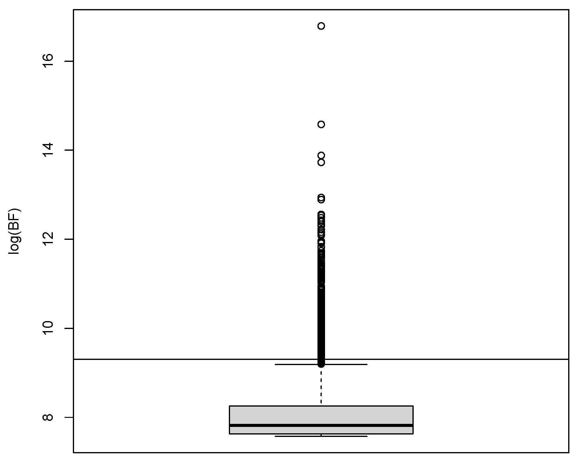
for $i=1,\dots ,n,$ and where the indexes of the variables are randomly selected and the covariates have been scaled so that the contribution of the parameter regression is similar in all the covariates. The standard deviation used for the errors mimics that observed in the real data. As expected, the true model here is highly endorsed by the simulated data, having a Bayes factor of 9.3 against the null, in logarithmic scale. Now, we have computed the Bayes factor of the models that result by adding a spurious covariate $x_j$ where $j\notin \{j_1,j_2,j_3,j_4,j_5\}$:

$$y_i={\beta }_0+{\beta }_{j_1}{x}_{j_{1}i}+{\beta }_{j_2}{x}_{j_{2}i}+{\beta }_{j_3}{x}_{j_{3}i}+{\beta }_{j_4}{x}_{j_{4}i}+{\beta }_{j_5}{x}_{j_{5}i}+{\beta }_j{x}_{ji}+{ϵ}_i,{ϵ}_i\sim N(0,{\sigma }^2).$$

There are $p-5=6092$ of these models whose Bayes factors are represented in Figure 1 in the form of a box-plot where the Bayes factor of the true model is also displayed. We see that there are a few number of models (6%) that surpass in evidence to the Bayes factor of the true model and some by an order of magnitude (the largest Bayes factor is almost 2000 times larger) and these would be eventually favoured in the variable selection scheme if for instance posterior probabilities are proportional to the Bayes factors. Notice that this is not an issue related with penalization for complexity since, if we were to compare only one of these models against the true model, the Bayes factor would, in the very great majority of occasions, successfully penalize complexity. The issue is because we are considering a huge amount of models and this fact should be taken into account. With the prior in Equation (4), the posterior probability of the wrong models to the true model would be approximately the ratio of Bayes factors times $p^{-1}$ so even the wrong model that provides the best fit would barely have 30% of the posterior probability of the true model.

Later we report that only two SNPs exhibit significant posterior inclusion probabilities, for the GWAS problem. This clearly differs from the results drawn by [24] where around 35 SNPs were declared important (the two most evidenced by the data being the two that we obtain). The approach in [24] is developed in two stages and multiplicity issues could be responsible for these disparate results.

The second consideration is of conceptual nature and concerns the existence of competing models $M_{\gamma }$ whose number of regressors, $k_{\gamma }+1$, exceed the sample size n. These are singular models in the sense that their parameters are not estimable because the design matrix is not of full row rank. There are a huge number of such models. For instance, in the GWAS dataset, the larger dimension of non-singular models is $k_{\gamma }=305$, entailing a proportion of around ${10}^{-1311}$ of the model space (hence, an upper bound of the proportion of non-singular models is ${10}^{-1308}$, in other words, the proportion of singular models is essentially one). It is clear that whatever we do with singular models may have a huge impact on the results. A popular possibility is to assign a zero prior probability to singular models (see, e.g., [25,26]). The severe dependence of the assumed prior, $p(M_{\gamma })$, on n is undesirable from a Bayesian perspective (seriously violating the principle of sequential updating). More importantly, from a practical perspective, is that one has to be aware of the strong underlying statement, namely that we are completely certain that the true number of covariates does not exceed n. In our problem, where $n=305$, this does not seem a compromising assumption but it could be so if the sample size was of the order of tens, as is the case of many omic studies.

In [27], the strategy to handle singular models is quite different, simply observing that these models provide a perfect fit, that is, $SS{E}_{\gamma }=0$ and can be reparameterized as models with $k_{\gamma }+1$ regression parameters. This results in Bayes factors equal to 1, like in the saturated models where $n=k_{\gamma }+1$. Once every $M_{\gamma }$ in the model space has a Bayes factor, we can combine these with $p(M_{\gamma })$ in Equation (4) to obtain the posterior distribution. With this simple approach the need for a prior $p(M_{\gamma })$ that depends on n disappears leading to a fully Bayesian methodology. Of course, it could be the case that the set of singular models, say ${\mathcal{M}}^S$, accumulates a probability. This situation, that would typically happen in cases where n is very small, would lead to non-informative results with highly multi-modal summaries and posterior inclusion probabilities of 0.5. Fortunately, we can asses the importance of the singular subset computing $p({\mathcal{M}}^S\mid \mathit{y})$. An estimation of this probability is provided in BayesVarSel. In the GWAS dataset, the estimation of $p({\mathcal{M}}^S\mid \mathit{y})$ is zero, hence confirming that here a sample size of $n=306$ is enough to ensure that the true model will be in the regular part of the model space.

The last consideration regards computational aspects of the problem. The model space is extremely large and, obviously, an exhaustive enumeration is unfeasible. Therefore, the question of how to approximate the posterior distribution arises. The Gibbs sampling, jointly with estimations based on the frequency of visits, was shown to be reliable for problems of moderate size in [15]. Assessing its performance when p is large (or very large) is still an open question and several authors (see, e.g., [28] and references therein) have argued about its possible limitations. Our position on this question is different and we believe that this simple sampling algorithm is a valid numerical tool for high dimensionality problems. A detailed study of this assertion would require a separate and comprehensive analysis that goes beyond the scope of this paper and will be considered in future research. Nevertheless, what it is always convincing is a comparison with the more recent methodologies to cope with scenarios of high dimensionality. One such method is the proposal in [29]—sparsevb—that replaces the actual posterior distribution with a variational approximation that allows for much faster computations. In their implementation, the authors use a spike-and-slab prior based on the Laplace density for the regression parameters and a prior over the model space that induces sparsity (favouring simpler models). Our main interest in the paper [29] is their comparison with a large number of competing Bayesian methods conceived for variable selection in high dimensional settings. In particular, they consider varbvs which is a related variational Bayes procedure but with the spike-and-slab prior using the Gaussian density. Additionally, ordinary (not-variational) spike-and-slab methods like the one based on an implementation of the Expectation Maximization algorithm [30] (called EMVS) and the more recent proposal in [31] (called SSLASSO) based on the well-known LASSO are considered. Finally, in the list of competing methods [29] also include the empirical Bayesian procedure (ebreg) in [32]. Notice that a method based on the popular BIC (Bayesian Information Criterion) is not an option in high dimensional settings because, as shown in [33], this criterion is too liberal with an inadequate tendency to favour complex models.

In the frequentist experiment in [29] they simulate 100 datasets from:

$$y_i=\sum _{j=1}^{380}{\beta }_j{x}_{ji}+\sum _{j=381}^p{\beta }_j{x}_{ji}+{ϵ}_i,{ϵ}_i\sim N(0,{\sigma }^2),i=1,2,\dots ,n$$

where $n=100$, $p=400$ and ${\beta }_j=0$ for $j=1,\dots ,380$ and ${\beta }_j=log(n)$ for $j=381,\dots ,400$ (only the last 20 variables are active). The error variance ${\sigma }^2=25$ and the covariates are simulated as iid standard normal variables. As it is common in the literature of variable selection, what is of most relevance in these type of simulated experiments is the frequency of times a given method provides the right response. This performance is normally summarized with two statistics: the false discovery rate (FDR, frequency of times an inert variable is declared as significant which in the Bayesian setting would correspond to an inclusion probability larger than 0.5) and the true positive rate (TPR, frequency of times a true explanatory variable is declared as irrelevant which in the Bayesian setting would correspond to an inclusion probability lower than 0.5). Obviously, methods with a FDR close to zero and TPR close to one are optimal. To summarize both statistics in only one, we also report the $F_1$ score, defined as the harmonic mean of the TPR and the Positive Predicted Value, PPV, determined by PPV=1-FDR. In the experiment described in [29], these statistics are computed and the results are reproduced in

Table 1. Simulation experiment in [29] for the different methodologies described in the text. In each of the 100 datasets, false discovery rate (FDR) is calculated as the number of inert variables ($1\le i\le 380$) not selected by the methodology, divided by the true number (380, in this case); FDR is reported as mean ± a Monte Carlo estimation of the standard error (estimated through the 100 replications). Similarly, TPR is calculated as the mean of the proportions for truly relevant variables ($381\le i\le 400$). $F_1$ score is the harmonic mean of true positive rate (TPR) and Positive Predicted Value (PPV) = 1-FDR.

	FDR	TPR	F1 Score
sparsevb	0.12 d ± 0.17	0.70 ± 0.31	0.78
varbvs	0.06 ± 0.11	0.34 ± 0.37	0.50
EMVS	0.24 ± 0.13	0.59 ± 0.14	0.66
SSLASSO	0.00 ± 0.00	0.01 ± 0.01	0.02
ebreg	0.38 ± 0.20	0.88 ± 0.18	0.73
Bayes	0.00 ± 0.00	0.99 ± 0.07	0.99

(cf. their Table 2) to which we have added those that correspond to our Bayesian methodology approximated with Gibbs sampling (that we simply label Bayes). This approach shows quite positive results although requiring a considerably greater computational burden: around 7 min per dataset as opposed to their computational time of less than a second.

Our experience on approximating the posterior distribution in the GWAS dataset (with a quite large p) can also be helpful to gain insight about the ability of the Gibbs sampling method. Initially, we ran the algorithm using the command GibbsBvs in BayesVarSel with $N={10}^4$ iterations and a burn-in of 1000 with three independent chains with initial models with one potential covariate randomly selected. In

Table 2. For GWAS dataset, results in several runs of the Gibbs sampling. In all cases, a burn-in of 1000 has been used and the intial model has 1 covariate randomly selected (for $N={10}^4$) and 10, 20 and 15 (randomly selected) in Chain 1, Chain 2 and Chain 3 (respectively) for $N=3\times {10}^4$. In parenthesis $B_{\gamma }(\mathit{y})p(M_{\gamma })$ (log scale) for the HPM found.

	N = 10,000						N = 30,000
	Chain 1		Chain 2		Chain 3		Chain 1		Chain 2		Chain 3
SNP	(22.49)		(26.01)		(19.23)		(26.52)		(25.46)		(26.52)
	ip	HPM	ip	HPM	ip	HPM	ip	HPM	ip	HPM	ip	HPM
rs10837540	1	y	1	y	1	y	1	y	1	y	1	y
rs11036238	1	y	1	y	1	y	1	y	1	y	1	y
rs7483683	0.51	y	0.53	n	0.48	n	0.51	n	0.46	n	0.52	y
rs357116	0.06	y	0.04	n	0.04	n	0.04	n	0.03	n	0.03	n
rs10160707	0.46	n	0.44	y	0.47	y	0.47	y	0.50	y	0.45	n
rs10017809	0.24	n	0.25	y	0.26	n	0.24	n	0.24	n	0.25	n
rs11242740	0.20	n	0.23	y	0.22	n	0.19	n	0.21	y	0.22	n
rs6844867	0.01	n	0.01	n	0.01	y	0.01	n	0.01	n	0.01	n

we have collected results for SNPs that have either an inclusion probability larger than 0.5 or was active in the HPM found. Despite the very large number p, there are only small disagreements on 6 variables. In this respect, the approximation of the inclusion probabilities are very similar for the chains agreeing in that only rs10837540 and rs11036238 have a substantial impact on the response. Of note, these are already known to be related to beta-thalassemia (rs10837540) or to be located near the HBB gene (rs11036238) and were also pointed out by [24]. We find slight variations about the best model encountered but these affect only few variables. To investigate the sensitivity of the method to the number of iterations we additionally ran the simulations for three chains now with $N=3\times {10}^4$ and initial models with 10, 20 and 15 SNPs randomly chosen. We clearly observe that the main conclusions remain the same and, quite remarkably, the inclusion probabilities are highly robust and barely vary. The HPMs found tend to be slightly simpler and with small variations between the chains (as a curiosity, we later discovered that SNPs rs10160707 and rs7483683 have exactly the same values). Finally, we also have computed the posterior probability (except for the normalizing constant) of the HPM model found in each chain (see Table 2). This value speaks about the “quality” of the models visited and it changes substantially in the different chains when $N={10}^4$ (the best model found in Chain 2 is 880 times more probable than that found by Chain 3) nevertheless, this aspect does not influence the goodness in the approximations of the main summaries of the posterior distributions. This observation clearly suggests the convenience of preserving the probabilistic structure of the problem when designing algorithms to explore the model space (as opposed to mechanisms to look for “good” models).

4. Variable Selection with Censored Data

4.1. The Real Problem

Longitudinal studies are very common in health sciences and, among other objectives, allow researchers to determine the risk factors that affect the course of a disease, the performance of a treatment, or determine whether a patient will suffer an adverse event. It is commonplace that these kind of studies deal with censored observations. In this framework, the variable selection problem for censored data naturally comes to light.

For illustration of the variable selection methodology with censored data we analysed data from a registry on acute coronary syndrome (ACS), which recruited patients from 10 hospitals between 2013 and 2017. See [34] for a detailed description of the study and the patients’ characteristics. The purpose of the study was to investigate the safety and efficacy (in terms of adverse events) of the treatment—a percutaneous coronary intervention (PCI) with a certain stent—in a clinical population with ACS. Patients entered the study in the date of the PCI and were followed up until the end of the study, time during which all major adverse cardiac events (MACE) are annotated. Although a lesion oriented outcome was the focus of the original study, in this application, we are interested in a composite endpoint—which we will refer to as MACE from now on—indicating whether the patient has died for cardiac causes, has suffered a myocardial infarction or has been revascularized during follow up, i.e., a patient oriented outcome.

Data of $n=1008$ patients with ACS who underwent a PCI were analysed. The dependent variable is, therefore, time to MACE in logarithmic scale. Free-of-events patients, at closing date, are treated as censored. There are $n_u=n-n_c=60$ uncensored observations, leading to a 94% of censoring.

The following potential explanatory variables were considered: age (years), sex, diabetes, hyperlipidemia, hypertension, current smoker, prior PCI, peripheral vascular disease, glomerular filtration rate (mL/min/1.73 m²), ST elevated MI (STEMI), unestable angina, left ventricular ejection fraction (%), multivessel disease, dual anti-platelet treatment (DAPT) period (months), DAPT with Clopidogrel (vs. Prasugrel or Ticagrelor), oral anticoagulation, stents implanted, total stent length (mm), and severe calcification (in any lesion).

4.2. Implementation of the Bayesian Approach

In this problem, the probability distribution $f_{\gamma }(\mathit{y}\mid {\beta }_0,{\mathit{\beta }}_{\gamma })$ is composed by two factors. The first factor comes from the uncensored data (i.e., those observations for which $y_i<c_i$), and is of the form in (5) and $N(·\mid \mu ,{\sigma }^2)$ denotes the density of a normal distribution with mean $\mu$ and variance ${\sigma }^2$. The second corresponds to the censored data and contributes to the distribution with the survival function:

$$S_{n_c}^{\gamma }(\mathit{c},{\beta }_0,X_c,{\mathit{\beta }}_{\gamma },\sigma )\equiv \prod _{i=1}^{n_c}{\int }_{c_i}^{\infty }N(t\mid {\beta }_0+{{\mathit{x}}_i}_{\gamma }^c{\mathit{\beta }}_{\gamma },{\sigma }^2)dt,$$

where ${{\mathit{x}}_i}_{\gamma }$ is the (transpose) of the i-th row vector of $X_c$ (the design matrix corresponding to the censored observations) for those variables active in $M_{\gamma }$. Also, slightly abusing notation c above represents the censored times for censored observations. With respect to the prior distributions, an obvious possibility would be adopting the conventional priors (6). Authors in [35] discuss in favour of this scheme but with a deep revision of the form of the variance matrix $V_{\gamma }$ (recall that this matrix is inspired by the information, in the sense of expected Fisher terms, that the sample contains about the parameters). These authors argue that the definition (7) is not adequate here since not all the observations contain, a priori, the same amount of information which in fact depends on the value of $c_i$. For instance, an observational unit with a very small $c_i$ will be very likely censored and its covariates ${\mathit{x}}_i$ should barely contribute to $V_{\gamma }$. These arguments are formally explored in [35] where it is shown that (7) in the censored problem leads to unsatisfactory results (like eg. violation of the predictive matching principle). Instead, [35] proposed using a weighted version of (7) that directly results from the analysis of the Fisher information matrix for this censored problem:

$$V_{\gamma }{({\beta }_0,\sigma )}^{-1}=\frac{{\sum }_{i=1}^{n}w(z_i)}{n}\sum _{i=1}^{n}w(z_i)({\mathit{x}}_{i\gamma }-{\overline{\mathit{x}}}_{w\gamma }){({\mathit{x}}_{i\gamma }-{\overline{\mathit{x}}}_{w\gamma })}^t,$$

(9)

where ${\overline{\mathit{x}}}_{w\gamma }={\sum }_{i=1}^{n}w(z_i){\mathit{x}}_{i\gamma }/{\sum }_{i=1}^{n}w(z_i)$, and $z_i$ is the standardization of $c_i$, that is $z_i=(c_i-{\beta }_0)/\sigma$ and

$$w(z)=\Phi (z)+\varphi (z)(\varphi (z)/(1-\Phi (z))-z),$$

where $\Phi ,\varphi$ stand for the cdf and pdf of a standard normal distribution. The properties of the weight function $w()$ are studied in [35] where it is shown that it behaves very similarly to a cumulative distribution function. Hence, the larger the standardized difference $(c_i-{\beta }_0)/\sigma$ (it is more likely that individual i is uncensored), the larger the value of the weight. In the limit, when $c_i\to -\infty$ ($c_i\to \infty$), $w_i\to 0$ ($w_i\to 1$). As a consequence, if all $c_i$ are equal then (9) and (7) coincide and, otherwise, the differences between the matrices will be more pronounced when the $c_i$ are more varying.

These weights are unknown because of its dependence on ${\beta }_0$ and $\sigma$. For the variable selection problem, this dependence is not an issue, as it is automatically handled in the computation of the marginal (2) via integration. Irrespectively of this, an inspection of the estimation of $w_i=w((c_i-{\beta }_0)/\sigma )$ can reveal interesting characteristics of the experiment. For instance, in the registry on ACS, the posterior means of $w_i$ (under $M_0$) vary moderately among the 1008 patients ranging from 0.02 to 0.33 with a mean of 0.25 and a standard deviation of 0.04. The values of the covariates that correspond to the patient with the lowest weight essentially will not contribute to the $V_{\gamma }$. That all the patients have a small estimated weight (recall weights are in the interval [0,1]) is due to very small censoring times in relation with the expected observed time and in fact only few persons are finally uncensored ($n_u=60$). In relation with this, an interesting quantity that arise within this approach is the sum ${\sum }_{i=1}^{n}w(z_i)$ that, following [36], can be interpreted as an effective sample size. That is, the equivalence in observed units of the censoring experiment. In the registry on ACS the posterior mean of the effective sample size under the null is 255 with a posterior standard deviation of 20. Hence, with the censoring mechanism used in this dataset, the $n=1008$ persons enrolled in the study count as 255 uncensored observations. Similarly, [37] analysed a penalization of the Bayesian Information Criterion (BIC) that takes into account that not all observations contribute equally to the likelihood when modelling censored data, implying that this definition of effective sample size could be used also in the context of BIC or other measures of variable selection.

For each competing model $M_{\gamma }$, the marginal density $m_{\gamma }(\mathit{y})$ now involves multivariate integrals in large dimensions (the subindex $\mathit{\gamma }$ has been removed to simplify notation):   

$$m(\mathit{y})=\int N_{n_u}(\mathit{y}\mid 1{\beta }_0+X_u\mathit{\beta },{\sigma }^{2}I)S_{n_c}(\mathit{c},{\beta }_0,X_c,\mathit{\beta },\sigma ){\sigma }^{-1}{N}_p(\beta \mid 0,g{\sigma }^{2}V({\beta }_0,\sigma ))h(g)d(g,\mathit{\beta },\sigma ,{\beta }_0).$$

Unlike the situation in the standard regression model, here the likelihood function does not conjugate with the prior because of the factor $S_{n_c}$. Also, as we already mentioned, the matrix V depends on ${\beta }_0,\sigma$. These two particularities make the computation of the marginal quite challenging and one has to envisage trustful ways to deal with such a multidimensional integral. Just to have an idea of the difficulty of computing $m(\mathit{y})$, the exact evaluation using importance sampling as described in Section 9 in [35] takes about 40 h for a problem with 6 covariates in a Linux machine with 32 parallel treads, making its implementation in the variable selection problem practically unfeasible (in the regression problem this takes a fraction of second). The alternative is to rely on a Laplace approximation, several authors have argued about the convenience of Laplace approximations over numerical approaches like for instance [38]. The only parameter that cannot be properly handled via Laplace integration is g, for that reason this parameter is integrated with standard numerical quadrature (for more details see Section 9 in [35]).

In this case, for the same problem with 6 covariates the approximation of all marginals takes 3 min (a sensible reduction). In our case the implementations in the entire variable selection problem that implies computing it in $2^{19}$ = 524,288 different models requires approximately 14 days to run. Quite obviously, to make the approach more broadly accessible we have to think on an implementation scheme that alleviate this computational burden. The idea is to perform a Gibbs sampling scheme to sample models over the model space then using the frequency of visits as an approximation to the posterior probability. This is of course a standard approach that is successfully implemented in the popular variable selection packages like BayesVarSel (see [22] for alternative R packages that implement related sampling schemes). Nevertheless in our problem, the main bottleneck is the computation of the marginal and we have to redesign the algorithm so that the computation of the Bayes factor is performed only the first time a model is sampled (and if is later resampled then the previous computation is used).

The Gibbs sampling algorithm begins taking an initial model ${\mathit{\gamma }}_{(0)}=({\gamma }_{1(0)},{\gamma }_{2(0)},\dots ,{\gamma }_{p(0)})$ with associated (Laplace) approximated Bayes factor $B_{{\gamma }_{(0)}}$ then repeating, for $i=1,\dots ,N$:

⋄

Step $j:1\le j\le p$. Consider the model ${\mathit{\gamma }}_{*}=({\gamma }_{1(i-1)},\dots ,1-{\gamma }_{j(i-1)},\dots ,{\gamma }_{p(i-1)})$. If this model has been sampled before, use its Bayes factor $B_{{\gamma }_{*}}$; otherwise, compute it and save it. Compute $r=B_{{\gamma }_{*}}p(M_{{\gamma }_{*}})/B_{{\gamma }_{(i-1)}}p(M_{{\gamma }_{(i-1)}})$ and with probability $min\{r,1\}$ re-define ${\mathit{\gamma }}_{(i-1)}={\mathit{\gamma }}_{*}$.

⋄

Final step. Define and save ${\mathit{\gamma }}_{(i)}={\mathit{\gamma }}_{(i-1)}$ and $B_{{\gamma }_{(i)}}p(M_{{\gamma }_{(i)}})$ (a quantity that is proportional to the posterior probability of this model).

The R code implementing this algorithm is provided as supplementary material. The approach is very efficient and produces very reliable results in a considerable shorter time. As an illustration, we describe the performance of this algorithm in the ACS dataset for which we ran the procedure with $N=$ 5000 taking around 20 h. The gain in time is essentially due to the fact that we only computed around 9500 different Bayes factors corresponding to the sampled models so only 2% of all models. For comparison, the estimated inclusion probabilities (through exhaustive enumeration) and their estimations using the Gibbs sampling are provided in

Table 3. Estimated inclusion probability based on exhaustive enumeration over the model space and using the Gibbs sampling algorithm for each variable.

Variable	Exhaustive Evaluation ip	Gibbs ip
Age	0.087	0.079
Sex	0.039	0.035
Diabetes	0.034	0.033
Hyperlipidemia	0.352	0.349
Hypertension	0.043	0.043
Current smoker	0.095	0.096
Prior PCI	0.132	0.123
Peripheral vascular disease	0.086	0.087
Glomerular filtration rate	0.054	0.053
STEMI	0.035	0.035
Unestable angina	0.035	0.033
Left ventricular ejection fraction	0.055	0.052
Multivessel disease	0.963	0.964
DAPT period	0.280	0.279
DAPT with Clopidogrel	0.068	0.063
Oral anticoagulation	0.089	0.084
Stents implanted	0.033	0.029
Total stent length	0.040	0.037
Severe calcification	0.031	0.031

, as it can be appreciated they are very similar.

4.3. Results

Table 4. Posterior probabilities of the more probable models, jointly with the BIC measure for these models.

Variables Included	Bayes Factor	Prior Prob.	Posterior Prob.	BIC
Multivessel dis.	293.09	0.003	0.312	525.58
Multivessel dis. + hyperlipidemia	724.12	0.0003	0.086	525.71
Multivessel dis. + DAPT period	389.5	0.0003	0.046	527.01
Multivessel dis. + hyperlipidemia + DAPT period	1725.87	0.00005	0.036	526.53

contains he Bayes factors, the prior probabilities and the posterior probabilities of the four more probable models. The HPM is the one that only includes multivessel disease, the second adds hyperlipidemia, the third considers variables multivessel disease and DAPT period, and the fourth model includes the three variables. We have also added the BIC defined using n in the penalization term. Results obtained with this definition of BIC are very similar to the ones reported by the posterior probability, the two more probable models are the ones with smaller BIC. However, BIC does not report any measure of uncertainty about the model selection by itself.

The posterior probabilities are, as expected, quite small since the number of models is very large. Perhaps posterior inclusion probabilities are more appealing and easier to interpret (see Table 3). In agreement with results in Table 4, only variable multivessel disease has a significant impact on the survival to a MACE. Also interesting is that there is barely any uncertainty in assessing that none of the other variables have any impact on the appearance of severe episodes of the studied disease.

The variable selection procedure, per se, does not provide the magnitude of the impact of a variable in the variable response. To answer this relevant question we must rely on Model Averaged estimations of the corresponding regression parameter. For illustration purposes, in Figure 2 we show the model averaged posterior distribution of ${\beta }_{Multivessel}$ with an estimated value of about −0.97 (its posterior mean) and a 95% credible interval of [−1.58, 0.54]. In terms of survival probabilities, straightforward computations show that patients with more than one affected vessel has probability of 0.86 of not experiencing a relapse after 5 years of the primary intervention (this probability is 0.95 for patients with none vessels affected).

5. Discussion

5.1. Theoretical Contributions and Practical Implications

The problem of variable selection arises frequently in health sciences research. Decisions made from these type of studies can have a great impact on society. The aim of this paper is to present the Bayesian approach for variable selection based on model choice, in practice, by showing its application to two common problems in health sciences. The first relates to genetics, aiming to link genes with a biomarker of a disease, in which a linear regression model is used, with a number of regressors that can be greater than the sample size. The second application is on a longitudinal study in cardiology, in the presence of censored data. Very little was found in the literature on the question of variable selection in these popular frameworks. One of the strengths of this paper is that goes beyond the standard regression model.

One of the key aspects of Bayesian variable selection is models’ prior selection. In Section 3, the results of this investigation show how multiplicity correction can be achieved by choosing a prior distribution over the model space. Regarding censored data, a prior that accounts for the amount of information provided by each individual in the sample is described in Section 4. The second major contribution was a fully Bayesian approach to deal with variable selection when $p\gg n$.

Both applications deal with a large model space, of which an exhaustive analysis is impractical. The results shown in Table 1 and Table 3 confirmed that the Gibbs sampling algorithm proposed for exploring the model space works satisfactorily.

5.2. Directions of Future Research

In order to summarise the results, the inclusion probability has been proved to be the most adequate measure to help practitioners in model choice. However, all the standard measures for summarising the results of variable selection are subject to certain limitations, when dealing with correlation in the covariates. This issue reasonably emerges in high dimensional problems, especially in genetics, as the set of possible values for the covariates is small. A reasonable approach to tackle this issue is described in [8]. Further research on dealing with covariates correlation would be worthwhile.

6. Conclusions

Overall, this research strengthens the idea that Bayesian variable selection can be applied to health sciences problems, providing a reliable tool to approach these problems. The findings of this study have a number of practical implications and contribute to the understanding of Bayesian methods for variable selection. We hope that this work will expand the use of these methods among medical researchers.

References

- Mirams, G.R.; Pathmanathan, P.; Gray, R.A.; Challenor, P.; Clayton, R.H. Uncertainty and variability in computational and mathematical models of cardiac physiology. J. Physiol. 2016, 594, 6833–6847. [Google Scholar] [CrossRef] [PubMed]
- Desboulets, L.D. A review on variable selection in regression analysis. Econometrics 2018, 6, 45. [Google Scholar] [CrossRef] [Green Version]
- Castillo, I.; Schmidt-Hieber, J.; van der Vaart, A. Bayesian linear regression with sparse priors. Ann. Stat. 2015, 43, 1986–2018. [Google Scholar] [CrossRef] [Green Version]
- Berger, J.O.; Pericchi, L.R. Objective Bayesian Methods for Model Selection: Introduction and Comparison. In Model Selection; Lecture Notes–Monograph Series; Institute of Mathematical Statistics: Beachwood, OH, USA, 2001; Volume 38, pp. 135–207. [Google Scholar] [CrossRef]
- Jeffreys, H. Theory of Probability, 3rd ed.; Oxford University Press: Oxford, UK, 1961. [Google Scholar]
- Kass, R.E.; Raftery, A.E. Bayes Factors. J. Am. Stat. Assoc. 1995, 90, 773–795. [Google Scholar] [CrossRef]
- Barbieri, M.M.; Berger, J.O. Optimal Predictive Model Selection. Ann. Stat. 2004, 32, 870–897. [Google Scholar] [CrossRef]
- Barbieri, M.; Berger, J.O.; George, E.I.; Ročková, V. The median probability model and correlated variables. Bayesian Anal. 2021, in press. [Google Scholar]
- Bayarri, M.J.; Berger, J.O.; Forte, A.; García-Donato, G. Criteria for Bayesian Model Choice with Application to Variable Selection. Ann. Stat. 2012, 40, 1550–1577. [Google Scholar] [CrossRef] [Green Version]
- Scott, J.G.; Berger, J.O. Bayes and Empirical-Bayes Multiplicity Adjustment in the Variable-Selection Problem. Ann. Stat. 2010, 38, 2587–2619. [Google Scholar] [CrossRef] [Green Version]
- Touloupou, P.; Alzahrani, N.; Neal, P.; Spencer, S.E.F.; McKinley, T.J. Efficient model comparison techniques for models requiring large scale data augmentation. Bayesian Anal. 2018, 13, 437–459. [Google Scholar] [CrossRef] [Green Version]
- George, E.I.; McCulloch, R.E. Approaches for Bayesian variable selection. Stat. Sin. 1997, 7, 339–373. [Google Scholar]
- Clyde, M.A.; Ghosh, J.; Littman, M.L. Bayesian Adaptive Sampling for Variable Selection and Model Averaging. J. Comput. Graph. Stat. 2011, 20, 80–101. [Google Scholar] [CrossRef]
- Berger, J.O.; Molina, G. Posterior Model Probabilities Via Path-Based Pairwise Priors. Stat. Neerl. 2005, 59, 3–15. [Google Scholar] [CrossRef]
- Garcia-Donato, G.; Martinez-Beneito, M.A. On Sampling strategies in Bayesian variable selection problems with large model spaces. J. Am. Stat. Assoc. 2013, 108, 340–352. [Google Scholar] [CrossRef]
- Bayarri, M.J.; García-Donato, G. Extending Conventional Priors for Testing General Hypotheses in Linear Models. Biometrika 2007, 94, 135–152. [Google Scholar] [CrossRef]
- Zellner, A.; Siow, A. Posterior Odds Ratio for Selected Regression Hypotheses. Bayesian Statistics 1; Bernardo, J.M., DeGroot, M., Lindley, D., Smith, A.F.M., Eds.; Valencia University Press: Valencia, Spain, 1980; pp. 585–603. [Google Scholar]
- Zellner, A. On Assessing Prior Distributions and Bayesian Regression Analysis with g-prior Distributions. In Bayesian Inference and Decision Techniques: Essays in Honor of Bruno de Finetti; Zellner, A., Ed.; Edward Elgar Publishing Limited: Cheltenham, UK, 1986; pp. 389–399. [Google Scholar]
- Kass, R.E.; Wasserman, L. A Reference Bayesian Test for Nested Hypotheses and its Relationship to the Schwarz Criterion. J. Am. Stat. Assoc. 1995, 90, 928–934. [Google Scholar] [CrossRef]
- García-Donato, G.; Forte, A. Bayesian Testing, Variable Selection and Model Averaging in Linear Models using R with BayesVarSel. R J. 2018, 10, 155–174. [Google Scholar] [CrossRef] [Green Version]
- Clyde, M. BAS: Bayesian Adaptive Sampling for Bayesian Model Averaging; R Package Version 1.4.3; 2017. Available online: https://cran.r-project.org/web/packages/BAS/ (accessed on 28 December 2020).
- Forte, A.; García-Donato, G.; Steel, M. Methods and Tools for Bayesian Variable Selection and Model Averaging in Normal Linear Regression. Int. Stat. Rev. 2018, 86, 237–258. [Google Scholar] [CrossRef] [Green Version]
- Cabras, S.; Castellanos, M.E.; Biino, G.; Persico, I.; Sassu, A.; Casula, L.; del Giacco, S.; Bertolino, F.; Pirastu, M.; Pirastu, N. A strategy analysis for genetic association studies with known inbreeding. BMC Genet. 2011, 12, 63–74. [Google Scholar] [CrossRef] [Green Version]
- Armero, C.; Cabras, S.; Castellanos, M.E.; Quirós, A. Two-Stage Bayesian Approach for GWAS with Known Genealogy. J. Comput. Graph. Stat. 2019, 28, 197–204. [Google Scholar] [CrossRef]
- Johnson, V.E.; Rossell, D. Bayesian Model Selection in High-Dimensional Settings. J. Am. Stat. Assoc. 2012, 107, 649–660. [Google Scholar] [CrossRef] [Green Version]
- Shin, M.; Bhattacharya, A.; Johnson, V.E. Scalable Bayesian variable selection using nonlocal priors densities in ultrahigh-dimensional settings. Stat. Sin. 2018, 28, 1053–1078. [Google Scholar] [PubMed] [Green Version]
- Berger, J.O.; García-Donato, G.; Martinez-Beneito, M.A.; Peña, V. Bayesian variable selection in high dimensional problems without assumptions on prior model probabilities. arXiv 2016, arXiv:1607.02993. [Google Scholar]
- Griffin, J.; Latuszynski, K.; Steel, M. In Search of Lost (Mixing) Time: Adaptive Markov chain Monte Carlo schemes for Bayesian variable selection with very large p. arXiv 2020, arXiv:1708.05678v3. [Google Scholar] [CrossRef]
- Ray, K.; Szabó, B. Variational Bayes for high-dimensional linear regression with sparse priors. J. Am. Stat. Assoc. 2020, 1–31. [Google Scholar] [CrossRef]
- Rockova, V.; George, E.I. EMVS: The EM approach to Bayesian variable selection. J. Am. Stat. Assoc. 2014, 506, 828–846. [Google Scholar] [CrossRef]
- Rockova, V.; George, E.I. The spike-and-slab LASSO. J. Am. Stat. Assoc. 2018, 521, 431–444. [Google Scholar] [CrossRef]
- Martin, R.; Tang, Y.; Walker, S. Empirical Bayes posterior concentration in sparse high-dimensional linear models. Bernoulli 2017, 23, 1822–1847. [Google Scholar] [CrossRef] [Green Version]
- Chen, J.; Chen, Z. Extended Bayesian information criteria for model selection with large model spaces. Biometrika 2008, 95, 759–771. [Google Scholar] [CrossRef] [Green Version]
- de la Torre Hernandez, J.M.; Moreno, R.; Gonzalo, N.; Rivera, R.; Linares, J.A.; Veiga Fernandez, G.; Gomez Menchero, A.; Garcia del Blanco, B.; Hernandez, F.; Benito Gonzalez, T.; et al. The Pt-Cr everolimus-eluting stent with bioabsorbable polymer in the treatment of patients with acute coronary syndromes. Results from the SYNERGY ACS registry. Cardiovasc. Revasc. Med. 2019, 20, 705–710. [Google Scholar] [CrossRef]
- Castellanos, M.E.; García-Donato, G.; Cabras, S. A model selection approach for Variable Selection with Censored Data. Bayesian Anal. 2021, 16, 271–300. [Google Scholar] [CrossRef]
- Berger, J.O.; Bayarri, M.J.; Pericchi, L.R. The Effective Sample Size. Econom. Rev. 2014, 33, 197–217. [Google Scholar] [CrossRef]
- Volinsky, C.T.; Raftery, A.E. Bayesian Information Criterion for Censored Survival Models. Biometrics 2000, 56, 256–262. [Google Scholar] [CrossRef] [PubMed]
- Sabanes, D.; Held, L. Hyper-g priors for generalized linear models. Bayesian Anal. 2011, 6, 387–410. [Google Scholar]
Figure 1.
For the first simulated experiment, based on the genome-wide association studies (GWAS) dataset, boxplot of the Bayes factors (in logarithmic scale and compared to the null) of models defined adding a spurious covariate to the true model. The horizontal line represents the (log) Bayes factor of the true model.
Figure 2.
Model averaged posterior distribution of represented as a histogram. In a darker colour the bar that corresponds to the probability of this variable being zero (which in this case is very low).