Non-Parametric Generalized Additive Models as a Tool for Evaluating Policy Interventions

Abstract

The interrupted time series analysis is a quasi-experimental design used to evaluate the effectiveness of an intervention. Segmented linear regression models have been the most used models to carry out this analysis. However, they assume a linear trend that may not be appropriate in many situations. In this paper, we show how generalized additive models (GAMs), a non-parametric regression-based method, can be useful to accommodate nonlinear trends. An analysis with simulated data is carried out to assess the performance of both models. Data were simulated from linear and non-linear (quadratic and cubic) functions. The results of this analysis show how GAMs improve on segmented linear regression models when the trend is non-linear, but they also show a good performance when the trend is linear. A real-life application where the impact of the 2012 Spanish cost-sharing reforms on pharmaceutical prescription is also analyzed. Seasonality and an indicator variable for the stockpiling effect are included as explanatory variables. The segmented linear regression model shows good fit of the data. However, the GAM concludes that the hypothesis of linear trend is rejected. The estimated level shift is similar for both models but the cumulative absolute effect on the number of prescriptions is lower in GAM.

1. Introduction

Although well-conducted randomized control trial experiments (RCTs) provide the most reliable evidence on the effectiveness of interventions, these are not always feasible for policy intervention analysis. RCTs involves randomly allocating participant units into two groups: the treament group which includes the participants who receive the intervention, and the control group. Selection bias and confounding variables are minimized due to randomization. Thus the differences between groups can be attributed to the intervention. However, when it comes to measuring the effect of policy interventions, there may be obstacled to the use of RCTS, such as economic obstacles (impact evaluation are costly) or political constraints (to give services to some groups and not to others can generate conflicts).

As alternative to RCTs, the interrupted time series analysis (ITSA) offers a quasi-experimental research design to measure the effect of an intervention when randomization is not possible [1]. In an ITSA, the observations on the outcome before and after the intervention are used to test immediate and gradual effects of the intervention. ITSA has been used in various fields, such as financial economics [2], health policies [3] and regulatory actions [4], to name but a few.

Segmented regression analysis is the recommended approach for analysing data from an ITSA [5,6]. It requires data which are are evenly spaced and have enought information before and after the intervention. Segmented regression analysis of interrupted times series data allows us to estimate immediate and gradual effects of the intervention on the outcome. Segmented regression analysis also allows us to assess whether factors other than the intervention could explain the change, controlling for factors such as seasonality or autocorrelation.

Segmented linear regression models have been the most widely used in practice. These models allow estimating the changes both in level and trend that follow an intervention. However, the assumption of linearity often may hold only over short intervals. Trends before and/or after the intervention may follow non-linear patterns, such as curvilinear trends. Some non-linear effects can be accommodated in linear models by using polynomial trends [7] or transformations of the dependent variable such as the logarithmic transformation [8]. Other non-linear trend structures may require other alternative models such as Box–Jenkins models [9]. However, the greater complexity in the specification and interpretation of this type of model has led to their less use [10].

Generalized Additive Models (GAMs) have been proposed as an alternative to characterize general non-linear regressions, without requiring the analyst to prespecify the form of the non-linear relationship [11]. Recently, Sullivan et al. [12] showed that GAMs can be useful for characterizing trends in longitudinal data collected in Single Subject (SS) designs. SS design is most often used in applied fields of psychology, education and human behaviour. SS design is a research design in which a single individual, or very small samples, is analyzed during a baseline period followed by an intervention that can change the outcome. This period can be followed by a return to baseline due to the removal of the intervention. This design can lead to a nonlinear relationship between time and outcomes that may not be easily detected using linear models.

In this paper, we assess whether the use of GAMs can be extended to estimate the impact of an intervention in any ITSA. Simulated data are used to evaluate the performance of the segmented linear regression models and GAMs in estimating the level change and the cumulative effect of an intervention. Data were simulated assuming linear and non-linear trends and the mean squared error (MSE) and the mean percentage error (MPE) are used to compare both methodologies. An illustrative example with real data is shown where the impact of the 2012 Spanish cost-sharing reform on pharmaceutical prescription on the volume of prescriptions dispensed from pharmacies is analyzed [13].

The rest of the paper is organized as follows. Section 2 describes the segmented linear regression models and GAMs applied to ITSA. Section 3 describes the simulation exercise where the process followed to simulate the data and the comparison of the results for both models are shown. Section 4 describes the application to real data. Finally, Section 5 deals with the discussion and the conclusion of the paper.

2. Methods

2.1. The Interrupted Time Series Design

In the ITSA, we have an observed outcome variable $Y_t$ measured at each equally-spaced time point t. $Y_t$ is exposed to the intervention in periods from $T_0+1$ to T and unexposed in periods from 1 to $T_0$. Suppose that $Y_t\left(1\right)$ and $Y_t\left(0\right)$ represent the outcome with and without the intervention, respectively, and $Y_t$ is given as follows:

$$Y_t=\left\{\begin{array}{cc}{Y}_t\left(0\right)& \mathrm{for}t=1,\dots ,T_0\\ Y_t\left(1\right)& \mathrm{for}t=T_0+1,\dots ,T\end{array}\right.$$

(1)

The intervention effect at time t is defined as the subtraction $Y_t\left(1\right)-Y_t\left(0\right)$ for $t=T_0+1,\dots ,T$, and the cumulative effect is defined as the sum of the intervention effects ${\sum }_{t=T_0+1}^T(Y_t\left(1\right)-Y_t\left(0\right))$. However the counterfactual $Y_t\left(0\right)$ is never observed for the post-intervention period, so the intervention effect is not observed in the data. To estimate the intervention effect, it is necessary to make an assumption regarding the outcomes that would have occurred in the absence of intervention. In a segmented regression analysis ([5]), separate levels and trends are estimated in each segment before and after the intervetion. Regression forecast for the post-intervention time period assuming the parameters of the pre-intervention period becomes an accurate option when counterfactual is not observed.

2.2. Segmented Linear Regression Models

A basic statistical method for ITSA is the segmented linear regression model. In a segmented linear regression, or a break–point model, each segment of the time series before and the intervention can have different levels and trends. The segmented linear regression allows the outcome of interest to evolve differently before and after the intervention. This approach controls for secular trends. A change in the level of the outcome after the intervention may constitute an abrupt intervention, and a change in trend shows a variation in the evolution of the series.

The specification of the linear regression is:

$$Y_t={\beta }_0+{\beta }_1·T_t+{\delta }_1·I_t+{\delta }_2·{TI}_t+u_t\mathrm{for}t=1,\dots ,T$$

(2)

where $T_t$, or trend variable, is the value of the time variable at moment t (takes values from 0 to $T-1$), $I_t$ is an indicator variable of the intervention that takes value 0 for the periods from 1 to $T_0$ and value 1 for the periods from $T_0+1$ to T, and the variable ${TI}_t$ is a sequential numbering of the time periods of the intervention, that takes value 0 for the pre-intervention period, and takes values from 0 to $T-T_0-1$ for the periods from $T_0+1$ to T. Following the definition in (1), the expressions $Y_t\left(0\right)$ and $Y_t\left(1\right)$ are:

$$Y_t\left(0\right)={\beta }_0+{\beta }_1·T_t+u_t\mathrm{for}t=1,\dots ,T_0\mathrm{and}$$

$$Y_t\left(1\right)=({\beta }_0+{\delta }_1)+{\beta }_1·T_t+{\delta }_2·{TI}_t+u_t\mathrm{for}t=T_0+1,\dots ,T$$

The linear regression analysis can accommodate additional structures that allow a more accurate estimate of the change in level and/or trend of the outcome due to the intervention, such as explanatory variables not affected by the intervention (or control variables), seasonality or serial correlation of the data. In this last case, when the errors are assumed to follow a first order autoregressive process AR(1), the linear regression model can be estimated using the Prais-Winsten method [14] which uses the generalized least-squares method. When the order of correlation is assumed to be higher, the coefficients can be estimated using the OLS estimator but Newey–West standard errors [15] are used to handle this autocorrelation.

2.3. Generalized Additive Models

Generalized additive models (GAMs) are extensions of general linear models in which the outcome depends linearly on smooth functions of some predictor variables. GAMs link the outcome variable with the independent variables using smoothing splines, which are piecewise polynomials joined together at locations in the data known as knots. There are different methods proposed by the literature for smoothing with respect to a predictor variable (cubic regression splines, p-splines, adaptive smoothing, etc.) but the choice of the smoother has not been analyzed in this paper and we used the default thin plate regression splines. They are the default smoothing for the package mgcv in R [16] because they are an optimal smoother given basis dimension/rank ([17]) and they are more flexible than the cubic smoothing splines [18]. Thin plate regression splines do not have knots but are more computationally costly to set up [16]. GAMs can be defined by the next equation:

$$Y_t={\beta }_0+\sum f_j\left(x_t\right)+u_t,$$

(3)

where $f_j$ is the smoothing spline for the independent variable $x_t$. The more knots in the GAM, the more piecewise polynomials that will be estimated and the better the fit of the model to the data. The optimal set of smoothing functions is obtained by minimizing the penalized sum of squares criterion (PSS) in:

$$PSS=\sum _{t=1}^T{\left[Y_t-{\beta }_0-\sum f_j\left(x_t\right)\right]}^2+\sum _j\lambda \int f_j^{″}{\left(z_j\right)}^{2}d{z}_j$$

(4)

where $\lambda \ge 0$ is a parameter that controls the trade–off between the model’s fidelity to the data and the function smoothness of f. A value of $\lambda =0$ results in the relatively minimum smoothing, whereas large values result in an extremely smoothed (i.e., linear in the limit) function. The optimal smoothing parameter is chosen by cross-validation.

GAMs can be useful for characterizing trends in longitudinal data when it is thought that change over time is non-linear but the exact nature of that nonlinearity is not known. In such a case, the independent variable $x_t$ would be a variable for time $T_t$. This work proposes to apply GAMs for evaluating policy interventions. The expression in (2) would be replaced by the expression:

$$Y_t={\beta }_0+s_1\left(T_t\right)+{\delta }_1·I_t+s_2\left({TI}_t\right)+u_t\mathrm{for}t=1,\dots ,T$$

(5)

where $s_1$ and $s_2$ are smoothing functions for each corresponding predictor. This model applies a smoothing function to both the secular trend ($T_t$) and to the sequential numbering of the time periods of the intervention ${TI}_t$. It implies that there may be a nonlinear data trajectory without the implementation of the intervention, as well as a (potentially different) nonlinear data trajectory after the intervention.

GAMs can also adjust for serial correlation of the data assuming a generalized additive mixed model. Smooths are specified as part of the fixed effects model formula, but the wiggly components of the smooth are treated as random effects. This approach allows correlated errors to be dealt with via random effects [19,20]. Control variables not affected by the intervention or seasonality can also be included in the equation assuming a linear or non-linear relationship with the outcome variable.

3. Simulation Analysis

3.1. Data Generation Process

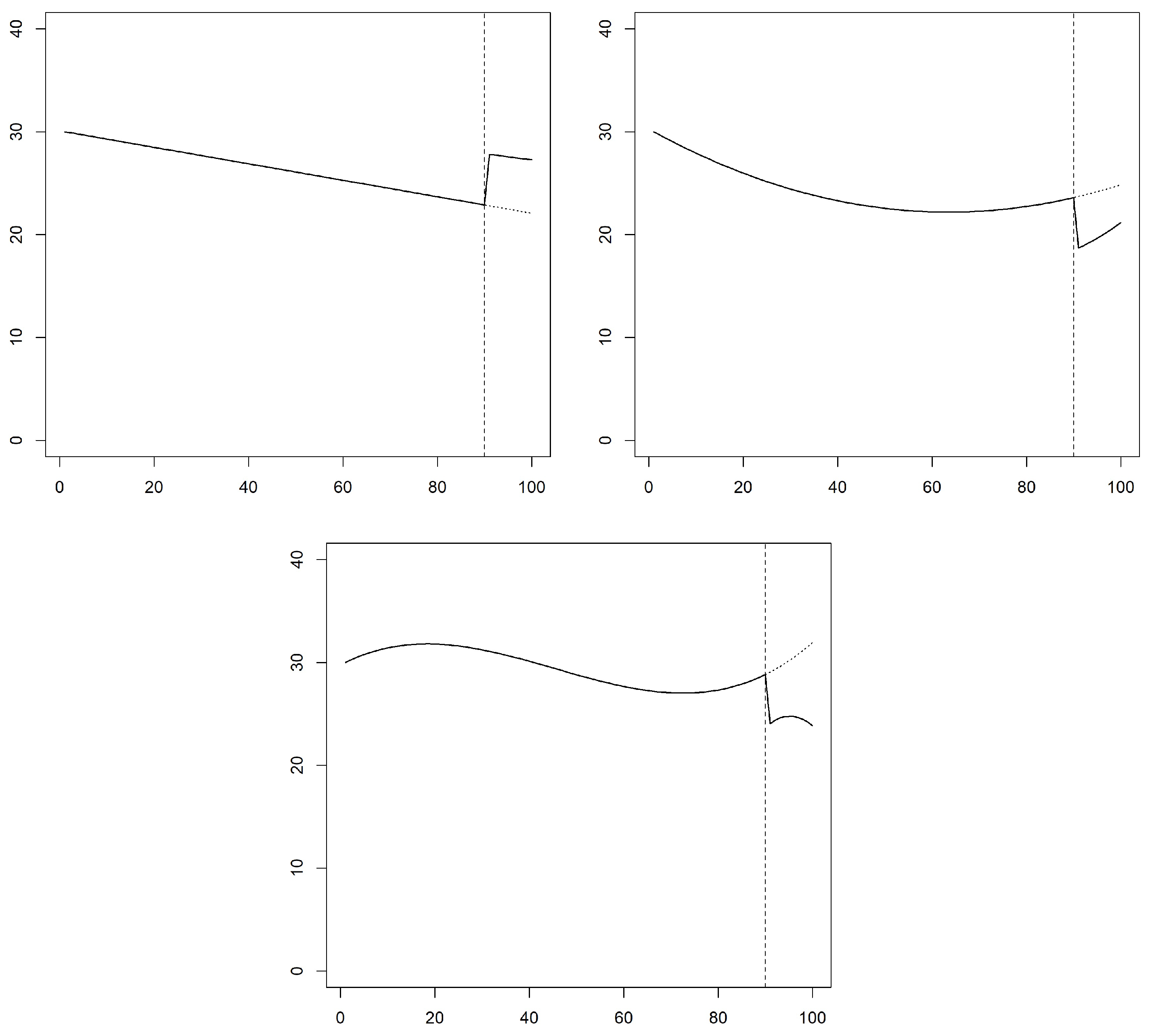
In this subsection we show how the simulated data were generated. For the sake of simplicity, we have assumed a fixed sample size of 100 for all time series, where the intervention affected the last 10 periods of the series. We have considered linear and non-linear trends before and after the intervention in the simulation process to study the performance of the segmented linear regression models and the GAMs in each of the cases. The number of simulations for each model was 500 and the possible autocorrelation in the series is considered assuming that the error term is distributed according to a first order autoregressive process AR(1) with parameter 0.3 and a standard deviation of the white noise process of 0.5.

The level change and the cumulative effect are analyzed and the performance of the models was evaluated through the comparison of estimated impacts of the intervention and the expected real impacts assumed in the simulation, using the mean squared error (MSE) and the mean percentage error (MPE).

The first simulation model assumes a linear but different trend before and after the intervention. It also assumes a change in the level of 5 units.

Table 1. Data generation.

Model	Specification	E [Immediate Impact]	E [Total Impact]
Linear model	$Y_t=30-0.08·T_t+5·I_t+0.02·T{I}_t+u_t$	5	50.9
Quadratic model	$Y_t=30-0.25·T_t+0.002·T_t^2-$ $-5·I_t+0.1·T{I}_t+0.005·T{I}_t^2+u_t$	$-5$	$-44.075$
Polynomial model	$Y_t=30+0.2235·T_t-0.008·T_t^2+0.00006·T_t^3-$ $-5·I_t+0.1·T{I}_t-0.05·T{I}_t^2+0.0001·T{I}_t^3+u_t$	$-5$	$-59.5475$

t varies from 1 to 100, $T_t$ is a sequential variable that takes values from 0 to 99; $I_t$ is an indicator variable that takes value 0 for the periods from 1 to 90 and value 1 for the periods from 91 to 100; $T{I}_t$ takes values 0 for period from 1 to 90 and takes values from 0 to 9 for the periods from 91 to 100; $u_t$ follows an AR(1) with parameter 0.3.

shows the parameters of this model. Figure 1 shows the deterministic part of the time series, where it is easily observed the assumed impact of the intervention through the comparison of the series before and after the intervention. The expected level change is 5 and the expected cumulative effect which includes the change in trend is 50.9 ($5·10+0.02·(0+1+2+\dots +9)$).

The second simulation model assumes a quadratic trend. Table 1 shows the parameters of this model and Figure 1 shows the deterministic part of the simulated data. In this case we have assumed a negative level change of $-5$ and an expected cumulative effect of −44.075.

Finally, the third simulation model assumes a cubic function. With this example we try to show a nonlinear model with several trend changes during the pre-intervention period. A cubic function can accommodate this behaviour. In practice a great majority of time series can be adequately fitted with polynomials with a maximum degree of 3 [21]. Table 1 and Figure 1 show the behaviour of this model, where the expected level change is assumed to be $-5$ and the expected cumulative effect is $-59.5475$.

The models have been estimated using the R statistical software, version 4.0.4. The codes are provided in the supplementary documents.

3.2. Results of the Simulation Analysis

Table 2. Results of the simulation analysis.

Simulation Model:	Linear Model		Quadratic Model		Polynomial Model
Level change
Estimated model:	SLRM	GAM	SLRM	GAM	SLRM	GAM
Mean (sd)	$5.0218\left(0.3935\right)$	$5.0246\left(0.4411\right)$	$-4.5442\left(0.6264\right)$	$-4.8969\left(0.4787\right)$	$-4.2842\left(0.6205\right)$	$-4.5857\left(0.5535\right)$
MSE	0.1550	0.1948	0.5993	0.2393	0.8966	0.4774
MPE	0.0627	0.0704	0.1273	0.0776	0.1594	0.1133
Cumulative effect
Estimated model:	SLRM	GAM	SLRM	GAM	SLRM	GAM
Mean (sd)	51.0629 (2.5283)	$51.1704\left(2.9021\right)$	$-23.6094\left(5.4400\right)$	$-40.5424\left(4.8718\right)$	$-36.0033\left(5.0288\right)$	$-49.8200\left(5.8647\right)$
MSE	6.4061	8.4787	448.3769	36.1665	579.5690	128.9503
MPE	0.0403	0.0449	0.4643	0.1119	0.3954	0.1698

SLRM: segmented linear regression model; GAM: generalized additive model; MSE: mean squared error; MPE: mean percentage error.

shows the results of the simulation analysis. Results include the mean and standard deviation of the level change estimated for the 500 simulations, along with the MSE and MPE obtained from the comparison with the expected level change for each simulation model. Similarly, the results for the cumulative effect are showed.

As expected, the segmented linear regression model obtains the best results for the linear simulation model. The mean level change is very close to the real expected level change (5.0218 and 5, respectively). The MSE is 0.1550 and the MPE is $6.27\%$. The mean cumulative effect is 51.0629 versus the real expected cumulative effect of 50.9. The MPE for the cumulative effect is $3.98\%$. Surprisingly, the GAM also obtains good results for the linear simulation model. The mean level change is 5.0246 although the dispersion is greater than that observed for the segmented linear regression model (0.4411 and 0.3935, respectively). The MPE for the level change is slightly higher, $7.04\%$. The results are similar for the estimation of the cumulative effect, where the MPE is $4.49\%$.

However, when the data are simulated from a non-linear model, the performance of the segmented linear regression model worsens. For the quadratic simulation model, the segmented linear regression model estimates a mean level change of $-4.5442$ when the real expected level change is $-5$. The MPE is $12.73\%$. The MPE for the cumulative effect is even greater, $46.43\%$. The flexibility of the GAM allows for a better fit for the non-linear simulation models. The mean estimated level change is $-4.8969$, very close to the real level change of $-5$. The good results of the GAM are maintained when estimating the cumulative effect. The mean cumulative effect is $-40.5424$ and the real cumulative effect is $-44.075$. The MPE is $11.19\%$.

For the more complex polynomial simulation model, the results of the GAM get worse, with an MPE of $11.33\%$ and $16.98\%$ for the estimation of the level change and the cumulative effect, respectively. However, these results are better than those obtained by the segmented linear regression model, where the MPEs are $15.94\%$ and $39.54\%$, respectively.

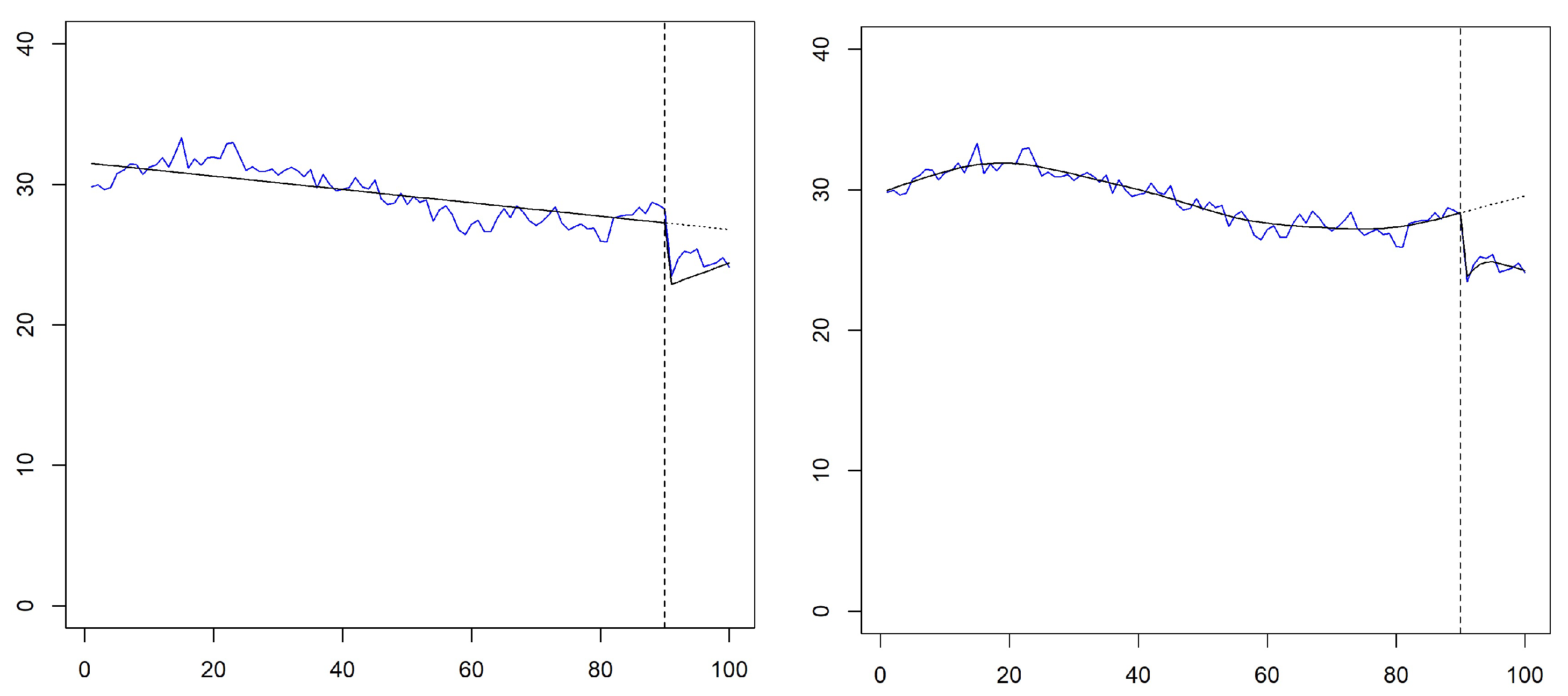
Figure 2 shows an illustrative example of how both models fit the same time series simulated from the polynomial model. The segmented linear regression model estimates a negative trend for the pre-intervention period. The level change is estimated at $-4.3307$, and the trend becomes a positive trend after the intervention, estimating a cumulative effect of $-33.5915$. The GAM fits a positive trend at the end of the pre-intervention period. The level change is now estimated at $-4.6535$. The estimated trend for the post-intervention period is lower than that observed before the intervention, and the cumulative effect is estimated at $-45.1620$.

4. Illustration with Real Data: Impact of the Cost-Sharing Reforms on Pharmaceutical Prescriptions Established in Spain

To illustrate the use of GAMs in a real-life application, we investigate the impact of the 2012 Spanish cost-sharing reforms on pharmaceutical prescription financed by the Spanish National Health Systems (SNHS) [13]. In June 2012 Spain enacted a reform of the co-payment for outpatient prescription drugs scheme, implemented early July 2012. Cost-free arrangements for all pensioners’ drugs were replaced by a $10\%$ co-payment subject to a monthly cap, depending on the income [22].

We use data relating to dispensed prescriptions for Pharmacies and financed by the SNHS. Data were collected from reports published by the Spanish Ministry of Health. We use monthly data from January 2004 to December 2015. The per-capita total prescription dispensed was calculated by dividing by the resident population of Spain.

The segmented linear regression model and GAM are applied to this dataset. Besides the level and trend before and after the intervention we have included as explanatory variables the seasonality (using indicator variables for the segmented linear regression model and a smoothing function for the GAM) and an indicator variable for the month previous to the intervention which examines the “stockpiling” effect between the announcement and the implementation of the law [23]. The codes are provided in the supplementary documents.

Table 3. Descriptive statistics of the per-capita prescriptions dispensed in Spain during the period 2004–2015.

	Pre-Intervention (2004–June 2012)	Post-Intervention (July 2012–2015)	2004–2015
Mean	1.6006	1.5429	1.5838
Median	1.6025	1.5599	1.5841
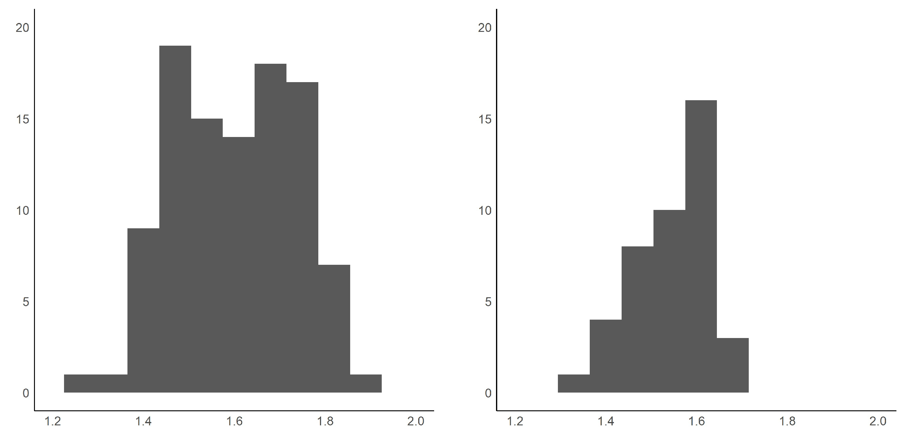
Standard deviation	0.0134	0.01222	0.0104

shows the descriptive statistics for the dependent variable for the pre- and post- intervention periods. The mean number of prescriptions decreased after the reform. The histogram plots of the per-capita prescriptions are shown in Figure 3. The Shapiro–Wilk normality tests confirm the normality hypothesis with p-values of 0.0806 and 0.1066 for the pre- and post- intervention periods, respectively.

Table 4. Results of the segmented linear regression model for real data.

Coefficients	Estimate (Standard Error)	p-Value
Intercept	1.4765 (0.0151)	<0.0001
$T_t$	0.0039 (0.0001)	<0.0001
$I_t$	−0.3068 (0.0138)	<0.0001
$T{I}_t$	−0.0012 (0.0005)	$0.0214$
Stockpiling	0.1117 (0.0477)	0.0207
January	reference
February	−0.0896 (0.0215)	<0.0001
March	−0.0324 (0.0188)	0.0871
April	−0.0500 (0.0195)	0.0115
May	−0.0373 (0.0194)	0.0559
June	−0.0676 (0.0198)	0.0009
July	−0.0978 (0.0194)	<0.0001
August	−0.2033 (0.0194)	<0.0001
September	−0.1207 (0.0194)	<0.0001
October	−0.0393 (0.0195)	0.0461
November	−0.0886 (0.0189)	<0.0001
December	−0.0723 (0.0214)	0.0010

shows the results of the segmented linear regression model. The level shift due to the new law is estimated at $-0.3068$, so the prescriptions per-capita decreased significantly as soon as the law was implemented. The upward trend of the series also decreases after the law in 0.0012 units. Combining both effects, the cumulative effect for the 42 months of law implementation is estimated in $-13.8856$ $[IC95\%$: $(-14.0628,-13.7085)]$. The rest of the coefficients shows a significant stockpiling effect, and a greater number of prescriptions during the month of January, compared to a lower number of prescriptions in the summer. The goodness of fit of the segmented linear regression model for these data is determined by an adjusted coefficient of determination of $0.9087$. The coefficient of the autoregresive model for the error term is estimated in $-0.2376$ and the residuals show a Durbin-Watson statistic of 2.007, showing that the Prais–Winsten estimation adequately controls for the autocorrelation.

Table 5. Results of the generalized additive model for real data.

	M1		M2
Coefficients	Estimate (Standard Error)	p-value	Estimate (Standard Error)	p-value
Intercept	1.6615 (0.0065)	<0.0001	1.6491 (0.0146)	<0.0001
$I_t$	$-0.2704$ (0.0198)	<0.0001	$-0.2704$ (0.0198)	<0.0001
Stockpiling	0.1604 (0.0471)	0.0009	0.1604 (0.0471)	0.0009
$T{I}_t$			0.0021 (0.0021)	0.3153
Smooth terms	EDF	p-value	EDF	p-value
$s\left(T_t\right)$	4.167	<0.0001	4.167	<0.0001
$s\left(T{I}_t\right)$	1.000	$0.315$
$s\left({month}_t\right)$	9.169	<0.0001	9.169	<0.0001

EDF: effective degrees of freedom.

shows the results of the GAM. The model M1 includes three coefficients: the intercept, an indicator variable for the intervention ($T_t$) and the indicator variable for the month before the intervention which refers to the stockpiling effect. Besides, the model includes three terms to be smoothed, the secular trend $s\left(T_t\right)$, the change in the trend after the intervention $s\left(T{I}_t\right)$ and the seasonality $s\left({month}_t\right)$. For this last smooth term, the maximum possible dimensions of the basis used for the spline is set to 12 ($k=12$), the number of months, while k is set by default as 9 for the rest of the smooth terms.

The level change is estimated in $-0.2704$ $[IC95\%$: $(-0.3096,-0.2312)]$, similar to that obtained by the segmented linear regression model, $-0.3068$. The stockpiling effect is statistically significant (p-value: 0.0009). The results for the smooth terms are summarized by the effective degrees of freedom (EDF), which measure the complexity of a penalized smooth term. EDF can be interpreted as an estimate of how many parameters are needed to represent the smooth [20]. If the EDF is equal to 1, a linear relationship cannot be rejected. In this analysis, the EDF is estimated at 4.167 for the secular trend showing its non-linearity. However, we cannot reject that the change in the trend after the intervention is linear. Seasonality is clearly non-linear. The cumulative effect is estimated at $-9.5623$ $[IC95\%$: $(-10.2504,-8.8742)]$, which is lower than that observed in the segmented linear regression model.

Due to the linearity of the $T{I}_t$ covariate, an alternative model M2, where $T{I}_t$ is included in the linear part of the model, is also shown in Table 5. Estimates do not vary and the variable $T{I}_t$ is not statistically significant. The cumulative effect is also estimated in $-9.5623$ $[IC95\%$: $(-10.2504,-8.8742)]$. The normality and unbiased error distribution were verified through four residual plots (using the command gam.check [16]). We also checked that the default maximum possible dimensions of the basis used for the trend spline ($k=9$) was enough.

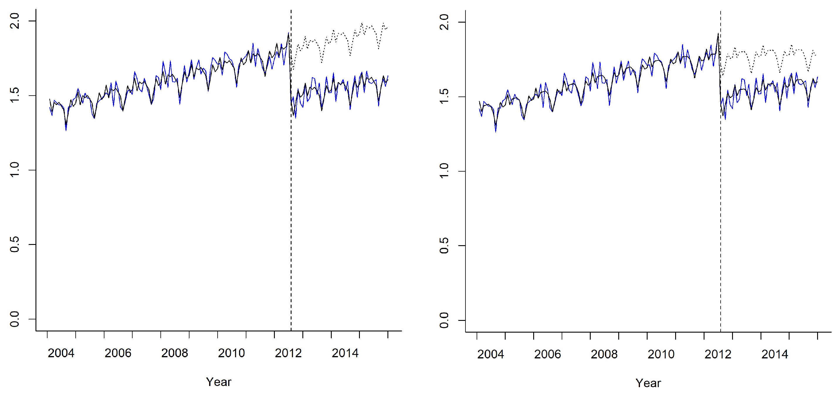
Figure 4 shows the fitted values for both models. The fits are similar, but the GAM predicts a lower trend for the post-intervention period if the intervention had not been performed, which leads to a smaller total impact. Even in this case where the linear model fits the data well, the difference in the total impact estimated by both models is statistically significant.

5. Conclusions

Interrupted time series analysis (ITSA) is a useful quasi-experimental design with which to evaluate the longitudinal effects of interventions. Its design is particularly useful for evaluating policy interventions. Segmented linear regression models have been the most used models to carry out this analysis. However, it may not be appropriate when trends are not linear and they cannot be transformed to be so.

In this paper, we show how generalized additive models (GAMs) [24,25,26,27] can be useful to accommodate nonlinear trends. GAM is a non-parametric regression-based method that can estimate non-linear trends in time series and can handle the irregular structure of some time series.

Our method generalizes the widely used regression methods applied to ITSA, which explicitly models the time series observed both before and after the intervention. The projection of the pre-intervention model for the post-intervention period can then be used as a counterfactual for the post-intervention period as if the intervention had not occurred.

The analysis with simulated data showed how GAMs improve on existing methods when the trend is non-linear, but they also show good performance when the trend is linear. The analysis with simulated data also showed how the segmented linear regression model fails as the trend model gets more complex. Other intervention effects, such as a pulse intervention, or other non-linear models for the trends, are also possible but we do not expect to observe different conclusions.

A real-life application where the impact of the 2012 Spanish cost-sharing reforms on pharmaceutical prescription is analyzed allows us to observe the differences that can be achieved when applying one or another methodology even in the case where the linear model fits the data well. GAMs also allow the inclusion of other explanatory (control) variables into the analysis assuming a linear or non-linear relationship with the outcome. In our example, the seasonality was included assuming a non-linear trend. The EDF has shown how the change in trend after the intervention ($T{I}_t$) could be modeled linearly. In that case, we recommend its inclusion in the linear part of the model due to its simplicity of estimation and interpretation. The autocorrelation in the error term can also be considered with GAMs which makes this method flexible enough to be applied in most situations.

In addition to GAMs, there are other alternative statistical methods for dealing with non-linear trends. These methods can be divided into two categories: the first includes regression methods like GAM such as the autoregressive integrated moving average (ARIMA) [10], and local regression (LOESS) [28]. The second category includes computing methods such as recurrent neural networks (RNN) [29], and other artificial intelligent systems. ARIMA models are usually considered robust for a long time-series only. These models have been used more in a predictive than an explanatory approach. To use ARIMA models we must to transform a time series into stationary one. ARIMA models are backward looking and not very flexible. Besides, ARIMA models are subjective and the reliability of the chosen model depends on the skill and experience of the researcher. Like GAMs, LOESS is a non-parametric regression method that fits a smooth line through data. But unlike LOESS, GAMs use flexible smoothing functions with automatic choice of smoothing parameteres. Finally, opacity is the most important disadvantage of RNN methods. Furthermore, training of RNN models can be difficult [30].

GAMs allow for model shapes from linear to nonlinear trends, a balanced reducing of model uncertainty, and the identification of time–periods of significant events [31]. However, the propensity to overfit is the main limitation of GAMs. Another limitation is that the model will lose predictability when the smoothed variables have values outside of the range of training dataset. GAMs are also restricted to be additive, thus important interactions can be missed. However, as with regular linear regression, we can manually add the interaction effects.

References

1. Shadish, W.R.; Cook, T.D.; Campbell, D.T. Experimental and Quasiexperimental Designs for Generalized Causal Inference; Houghton Mifflin: Boston, MA, USA, 2002. [Google Scholar]
2. Ho, A.K.F.; Wan, A.T.K. Testing for covariance stationarity of stock returns in the presence of structural breaks: An intervention analysis. Appl. Econ. 2002, 9, 441–447. [Google Scholar] [CrossRef]
3. Lagarde, M. How to do (or not to do)... Assessing the impact of a policty change with routine longitudinal data. Health Policy Plan. 2012, 27, 76–83. [Google Scholar] [CrossRef] [PubMed] [Green Version]
4. Briesacher, B.A.; Soumerai, S.B.; Zhang, F.; Toh, S.; Andrade, E.; Wagner, J.L.; Shoaibi, A.; Gurwitz, J.H. A critical review of methods to evaluate the impact of FDA regulatory actions. Pharmacoepidemiol. Drug Saf. 2013, 22, 986–994. [Google Scholar] [CrossRef] [PubMed] [Green Version]
5. Wagner, A.K.; Soumerai, S.B.; Zhang, F.; Ross-Degnan, D. Segmented regression analysis of interrupted time series studies in medication use research. J. Clin. Pharm. Ther. 2002, 27, 299–309. [Google Scholar] [CrossRef] [PubMed]
6. Taljaard, M.; McKenzie, J.E.; Ramsay, C.R.; Grimshaw, J.M. The use of segmented regression in analysing interrupted time series studies: An example in pre-hospital ambulance care. Implement. Sci. 2014, 9, 77. [Google Scholar] [CrossRef] [PubMed] [Green Version]
7. Gillings, D.; Makuc, D.; Siegel, E. Analysis of interrupted time series mortality trends: An example to evaluate regionalized perinatal care. Am. J. Public Health 1981, 71, 38–46. [Google Scholar] [CrossRef] [PubMed] [Green Version]
8. McCleary, R.; McDowall, D.; Bartos, B. Design and Analysis of Time Series Experiments; Oxford University Press Inc.: New York, NY, USA, 2017. [Google Scholar]
9. McDowall, D.; McCleary, R.; Meidinger, E.E.; Hay, R.A. Interrupted Time Series Anlaysis; Sage: Newbury Park, CA, USA, 1980. [Google Scholar]
10. Hategeka, C.; Ruton, H.; Karamouzian, M.; Lynd, L.D.; Law, M.R. Use of interrupted time series methods in the evaluation of health system quality improvement interventions: A methodological systematic review. BMJ Glob. Health 2020, 5, e003567. [Google Scholar] [CrossRef] [PubMed]
11. Hastie, T.; Tibshirani, R. Generalized Additive Models; John Wiley & Sons, Inc.: Hoboken, NJ, USA, 1990. [Google Scholar]
12. Sullivan, K.J.; Shadish, W.R.; Steiner, P.M. An introduction to modeling longitudinal data with generlaized additive models: Applications to single-case designs. Psychol. Methods 2015, 20, 26–42. [Google Scholar] [CrossRef] [PubMed] [Green Version]
13. Puig-Junoy, J.; Rodríguez-Feijoó, S.; López-Valcárcel, B.G. Paying for formerly free medicines in Spain after 1 year of co-payment: Changes in the number of dispensed prescriptions. Appl. Health Econ. Health Policy 2014, 12, 279–287. [Google Scholar] [CrossRef] [PubMed]
14. Prais, S.J.; Winsten, C.B. Trend Estimators and Serial Correlation; Working paper 383; Cowles Commission: Chicago, IL, USA, 1954. [Google Scholar]
15. Turner, S.; Karahalios, A.; Forbes, A.B.; Taljaard, M.; Grimshaw, J.M.; Cheng, A.C.; Bero, L.; McKenzie, J.E. Design characteristics and statistical methods used in interrupted time series studies evaluating public health interventions: A review. J. Clin. Epidemiol. 2020, 122, 1–11. [Google Scholar] [CrossRef] [PubMed]
16. Wood, S. Package “mgcv”. Mixed GAM Computation Vehicle with Automatic Smoothness Estimation. R package version 1.8-33. 2020. Available online: https://cran.r-project.org/web/packages/mgcv/mgcv.pdf (accessed on 26 January 2021).
17. Wood, S.N. Thin plate regression splines. J. R. Stat. Soc. Ser. B 2003, 65, 95–114. [Google Scholar] [CrossRef]
18. Perperoglou, A.; Sauerbrei, W.; Abrahamowicz, M.; Schmid, M. A review of spline function procedures in R. BMC Med. Res. Methodol. 2019, 19, 46. [Google Scholar] [CrossRef] [PubMed] [Green Version]
19. Wood, S. Low rank scale invariant tensor product smooths for generalized additive mixed models. Biometrics 2006, 62, 1025–1036. [Google Scholar] [CrossRef] [PubMed] [Green Version]
20. Wood, S. Generalized Additive Models: An Introduction with R; Taylor and Francis: Boca Raton, FL, USA, 2006. [Google Scholar]
21. Van Gellecom, F.S. Advances in non-linear economic modeling-theory and applications. In Dynamic Modeling and Econometrics in Economics and Finance; Springer: Berlin/Heidelberg, Germany, 2014; Volume 17. [Google Scholar]
22. Official State Bulletin (BOE). Urgent Measures to Guarantee the Sustainability of the National Health System and Improve the Quality and Safety of Services; Royal Decree Law (RDL) 16/2012; BOE: Madrid, Spain, 2012. [Google Scholar]
23. Hernandez-Izquierdo, C.; López-Valcárcel, B.G.; Morris, S.; Melnychuk, M.; Abásolo, I. The effect of a change in co-payment on prescription drug demand in a National Health System: The case of 15 drug families by price elasticity of demand. PLoS ONE 2019, 14, E0213403. [Google Scholar]
24. Hastie, T.; Tibshirani, R. Generalized Additive Models. Stat. Sci. 1986, 1, 297–318. [Google Scholar] [CrossRef]
25. Yee, T.W.; Mitchell, N.D. Generalized additive models in plant ecology. J. Veg. Sci. 1991, 2, 587–602. [Google Scholar] [CrossRef]
26. Ruppert, D.; Wand, M.P.; Carroll, R.J. Semiparametric Regression; Cambridge University Press: Cambridge, UK, 2003. [Google Scholar]
27. Wood, S. Generalized Additive Models and Introduction with R, 2nd ed.; Chapman and Hall/CRC: London, UK, 2017. [Google Scholar]
28. Wasserman, L. All of Nonparametric Statistics; (Springer Texts in Statistics); Casella, G., Fienberg, S., Olkin, I., Eds.; Springer: New York, NY, USA, 2006; Chapter 5; pp. 61–123. [Google Scholar]
29. Hewamalage, H.; Bergmeir, C.; Bandara, K. Recurrent Neural Networks for Time Series Forecasting: Current Status and Future Directions. Int. J. Forecast. 2020, 37, 388–427. [Google Scholar] [CrossRef]
30. Levin, E. A recurrent neural network: Limitations and training. Neural Netw. 1990, 3, 641–650. [Google Scholar] [CrossRef]
31. Simpson, G.L. Modelling Palaeoecological Time Series Using Generalised Additive Models. Front. Ecol. Evol. 2018, 6, 149. [Google Scholar] [CrossRef] [Green Version]
Figure 1. Simulated data. The left upper plot shows the linear model, the right upper plot shows the quadratic model and the lower plot shows the polynomial model. In all pictures, the black line refers to the deterministic part of the simulated data, and the dashed line refers to the projection of the pre-intervention model in the post-intervention period.
Mathematics 09 00299 g001
Figure 2. Results for simulated data. The left plot shows the segmented linear regression analysis and the right plot shows the generalized additive analysis. In both pictures, the blue line refers to the simulated data, the black line refers to the fitted values and the dashed line refers to the projection of the pre-intervention model in the post-intervention period.
Mathematics 09 00299 g002
Figure 3. Histogram plots of the per-capita prescriptions for the pre-intervention period (left plot) and the post-intervention period (right plot).
Mathematics 09 00299 g003
Figure 4. Results for real data. The left plot shows the segmented linear regression analysis and the right plot shows the generalized additive analysis. In both pictures, the blue line refers to the simulated data, the black line refers to the fitted values and the dashed line refers to the projection of the pre-intervention model in the post-intervention period.
Mathematics 09 00299 g004