
An Intuitionistic Fuzzy Set Driven Stochastic Active Contour Model with Uncertainty Analysis


School of Electronic Engineering, Xidian University, Xi’an 710071, China
*
Author to whom correspondence should be addressed.
Mathematics 2021, 9(4), 301; https://doi.org/10.3390/math9040301
Submission received: 8 January 2021
/
Revised: 29 January 2021
/
Accepted: 29 January 2021
/
Published: 3 February 2021
(This article belongs to the Special Issue Fuzzy Sets and Soft Computing)
Abstract
:Image segmentation is a process that densely classifies image pixels into different regions corresponding to real world objects. However, this correspondence is not always exact in images since there are many uncertainty factors, e.g., recognition hesitation, imaging equipment, condition, and atmosphere environment. To achieve the segmentation result with low uncertainty and reduce the influence on the subsequent procedures, e.g., image parsing and image understanding, we propose a novel stochastic active contour model based on intuitionistic fuzzy set, in which the hesitation degree is leveraged to model the recognition uncertainty in image segmentation. The advantages of our model are as follows. (1) Supported by fuzzy partition, our model is robust against image noise and inhomogeneity. (2) Benefiting from the stochastic process, our model easily crosses saddle points of energy functional. (3) Our model realizes image segmentation with low uncertainty and co-produces the quantitative uncertainty degree to the segmentation results, which is helpful to improve reliability of intelligent image systems. The associated experiments suggested that our model could obtain competitive segmentation results compared to the relevant state-of-the-art active contour models and could provide segmentation with a pixel-wise uncertainty degree.
1. Introduction
Image segmentation is an important technology in computer vision, and it has been widely applied to many fields [1,2,3]. It essentially is a process to extract image objects according to human recognition in the real world. Many factors, however, e.g., human recognition, digital imaging equipment, imaging condition, and atmospheric environment, usually result in inconsistency in image feature and uncertainty in recognition. These also put great challenges on image segmentation, parsing, and recognition. For example, Google identified Africans as chimpanzees, Flickr identified concentration camps as gyms, and Uber’s autonomous vehicles killed a pedestrian. These unfortunate accidents called extensive attention from academia and industry. To avoid the aforementioned accidents, we model the uncertainty in segmentation via intuitionistic fuzzy set and design a novel energy functional for stochastic active contour model (ACM) to realize a segmentation with low uncertainty.
In the past three decades, due to the flexible and accurate representation of object boundaries, ACMs have attracted extensive attention in image segmentation. The earliest ACM, proposed by Kass et al. and named Snakes [4], used parametric equations to implicitly represent closed planar curves, and suffered from the inefficiency of handling topology changing, i.e., emerging and splitting of curves. To overcome this problem, Osher and Sethian [5] proposed an implicit ACM, i.e., level set method (LSM). It employed the zero level set of a signed distance function to describe planar curves, which greatly facilitates the handling of curves’ topology changes. After that, most ACMs basically followed this implicit representation for planar curves. Caselles et al. proposed an edge-based LSM inspired by geodesics active contour model [6] to avoid boundary leakage caused by the stopper function based on image gradient. This method, however, is sensitive to initial curves. Mumford and Shah [7] proposed a smooth image approximation for segmentation; however, its computation cost is pretty high. Simplifying this model by a piecewise constant function for the image approximation, Chan and Vese proposed a region-based LSM, called CV model [8], to extract objects without clear boundaries, but it could not obtain the desired result on inhomogeneous images. Aiming at this problem, many improved LSMs have been proposed; for example, Tsai et al. [9] adopted piecewise smooth function instead of piecewise constant function to approximate images, Li et al. proposed Local Binary Fitting model (LBF) [10] and a Region-Scalable Fitting (RSF) energy functional [11] to locally approximate inhomogeneous images, and Zhang et al. proposed a Local Image Fitting model (LIF) [12]. In addition, many scholars combined ACMs with fuzzy logic to improve segmentation accuracy. Gibou et al. [13] proposed a fast LSM with K-means to handle blur images. Chen et al. combined fuzzy clustering method with geodesic active contour model and applied it to magnetic resonance (MR) images [14]. Krinidis and Chatzis proposed a Fuzzy Energy-Based Active Contour (FEBAC) model [15]. Then, Tran et al. [16] added a shape-prior to fuzzy energy that improves the segmentation effectiveness on images with clutter background and object occlusion. In brief, currently, most ACMs basically focus on harnessing more image features or finding more reasonable appearance model for the data-driven functional terms.
ACMs essentially utilize Partial Differential Equations (PDEs) designed in advance to drive planar curves approaching object boundaries in images. PDEs, however, being a kind of deterministic physical equation, form a contradiction with the randomness in real images. Considering the disability of PDEs, many scholars, hence, introduced Stochastic Differential Equations (SDEs) to evolve curves and proposed Stochastic ACM [17]. After the concept of stochastic integral was put forward by Itô, SDEs have gradually become an important mathematical tool for systematic quantitative analysis and stochastic phenomena. It has been extensively used in physics, chemistry, electronic engineering, etc. [18]. Juan et al. proposed an ACM on Stratonovich SDEs for image segmentation, which greatly improved the segmentation performance against noise [17]. Law et al. proposed a hybrid approach which combines gradient based method and stochastic optimization method to find the global optimal solution [19]. Dariusz et al. adopted the backward stochastic differential equation to reconstruct images, which could smoothen images and sharpen image edges as well [20]. Hedges et al. proved that deterministic algorithms easily get trapped in local extremes in non-convex optimization problem and proposed a method for stochastic shape optimization of engineering structures [21]. Due to the outstanding intrinsic features, SDEs possess potential and play more and more important role in different tasks.
Fuzzy set proposed by Zadeh is a kind of soft computing methods that is suitable for solving the scientific problems having no exact solutions [22]. Soft computing made dramatic progress and wide application in recent years and is composed of various methods: fuzzy logic, neural networks, genetic algorithm, etc. Attanassov proposed an intuitionistic fuzzy set (IFS) to model the hesitation when people make a determination [23]. Xuan et al. proposed a support IFS in which an element has three membership functions in a given set and defined new operators on membership functions [24]. Song et al. proposed a new similar measure of membership functions and applied it to clustering analysis and medical diagnosis [25]. Riaz, e.g., analyzed the properties of soft multi-set topology and proposed multi-criteria decision-making algorithms with aggregation operators [26]. Sahoo et al. presented a soft computing neural networks tool based on radial function networks and studied the problem of transmission line congestion in electrical power systems [27]. Das et al. reviewed several types of support vector machine based methods in data mining and compared and analyzed various methods and techniques [28]. Rzheutskaya et al. employed genetic programming to generate an appropriate classification tree [29]. Zhang et al. proposed a new optimized method to automatically select edge servers in mobile edge environment via combining genetic algorithm and simulated annealing algorithm [30].
In summary, image segmentation is an ill-posed problem, and people usually classify pixels into different categories according to their different recognition. Meanwhile, many factors, e.g., imaging equipment and condition as well as atmosphere environment, also accentuate this uncertainty, which results in segmentation results full of uncertainty. Considering the great progress of ACM in recent years, we leverage IFS to model this uncertainty, and firstly introduce it into stochastic ACM by designing a new energy functional. By optimizing this functional, we realize image segmentation with low uncertainty. In addition, we also achieve the relevant uncertainty degree as a co-product of segmentation. The proposed method possesses the following advantages: (1) more competitive segmentation performance on complex images; (2) segmentation results with low uncertainty; and (3) the ability to cross saddle points when optimizing the energy functional. The proposed method benefits to the subsequent procedures of computer vision, e.g., image parsing and image understanding, due to the segmentation result with low uncertainty. The experiments also suggest that our method could achieve promising segmentation results as well as the uncertainty degree of segmentation as a co-product.
The remainder of this paper is organized as follows. Section 2 briefly revisits a few representative ACMs related to our model. In Section 3, the proposed method is expounded including the generation of stochastic images, designing of the energy functional based on IFS, and optimization of the energy functional in detail. Section 4 verifies our method against the state-of-the-art ACMs on different images. Finally, Section 5 presents a conclusion of our work.
2. The Previous Works
Given an image on a domain where , Chan and Vese [8] adopted a piece-wise constant function to approximate the intensity distribution of two regions inside and outside the closed curve , respectively. The associated energy functional is defined as
where , and are empirical positive parameters. is a signed distance function referred to as hereinafter. is Heaviside function and is its derivative function, i.e., Dirac function. represents the region inside the closed curve C, and the region outside C. and are the average values of the pixels’ grayscale inside and outside C, respectively. When fixing , we could update these two parameters by
This model is insensitive to noise, and could obtain good performance on blur images. However, it could not well handle inhomogeneous images due to using a piece-wise constant function to approximate segmentation. Li et al. proposed an ACM named RSF that drew upon intensity information in local regions at a controllable scale [11]. Its energy functional is defined as
where is a Gaussian kernel with standard deviation . Instead of and in (1), and are the functions of , and they denote the prototypes for the regions inside and outside the closed curve , respectively. These two functions could be updated by
This method could achieve better performance on inhomogeneous images compared with CV method [8]. It, however, could not well handle the images with rich texture and complex background; it also easily gets stuck in the local extremes of the energy functional. Additionally, Niu et al. proposed a novel region-based ACM for segmentation of objects by introducing a local similarity regularization, naming it RLSF [31]. The energy functional is formulated as
where is the neighborhood of the point and is a spatial Euclidean distance between the pixel and the center . and represent the intensity means in the local interior and exterior regions centered at the pixel , which can be computed by
where the mask is an indicator function for a local region. This method utilizes prototype functions to depict object and background, i.e., (6). similar to RLSF [31]. It, however, brings a pretty heavy computation cost as well as makes a more precise representation.
Krinidis and Chatzis [15] combined ACM with fuzzy set to make the FEBAC model and proposed a fuzzy-based energy function defined as
where the membership function is the degree of the pixel belonging to the region inside the curve C denoted by . Keeping fixed, we can update and in a similar way as (2). Keeping and fixed, the membership degree function can be updated by
The fuzzy energy terms contribute to dealing with blurriness and inhomogeneity in images and make the model robust against initial curves.
3. The Proposed Stochastic ACM
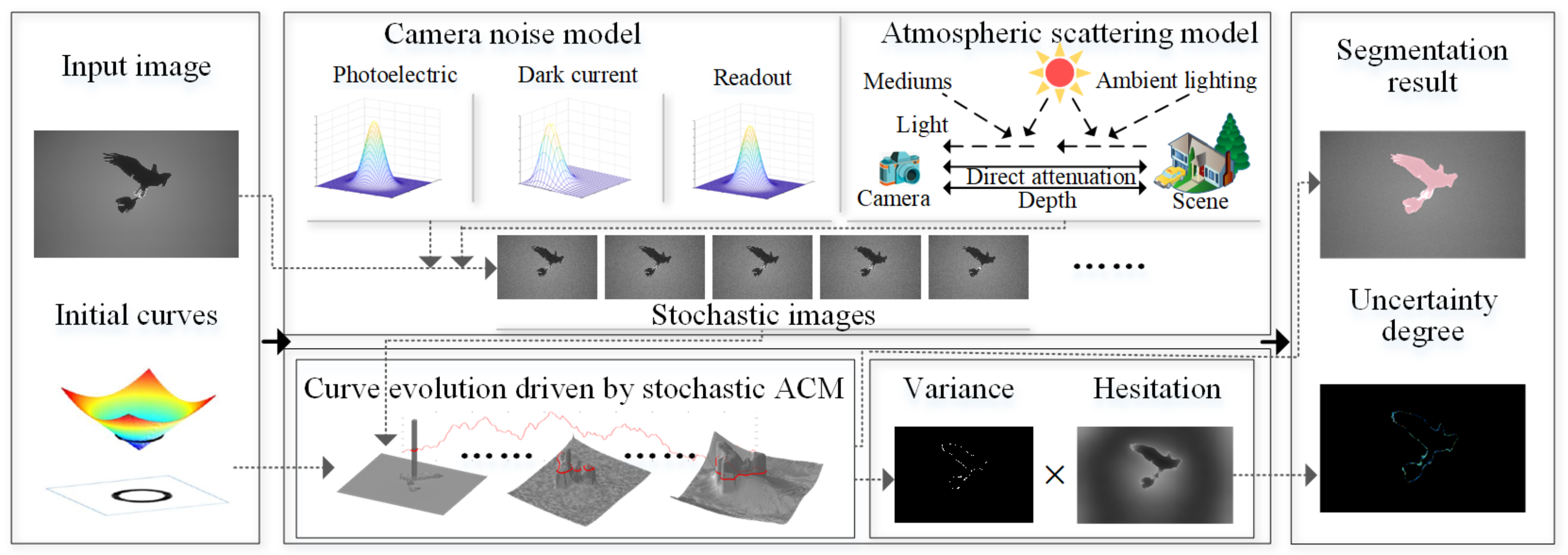
In this section, we detail the proposed stochastic ACM including its energy functional, the evolution equation, and the uncertainty measurement of segmentation. Our model utilizes Stochastic Partial Differential Equation (SPDE) to handle the uncertainty of data, employs IFS to simulate the recognition uncertainty, and provides segmentation result with uncertainty degree. The general architecture is illustrated in Figure 1.
In our model, one image is taken as input, and it is utilized to generate a series of images by several stochastic processes to model the effect from digital imaging equipment as well as atmospheric environment. The stochastic active contour model with the energy term based on intuitionistic fuzzy set drives the initial surface/curve approaching the object boundaries. When iteration is over, the variance of the final results on stochastic images and the hesitation degree from IFS are combined to be an uncertainty degree about segmentation.
3.1. The Generation of Stochastic Images
Acquisition devices, imaging condition, and atmospheric environment all result in inevitable randomization of imaging, which herein are numerically simulated by some stochastic distribution according to the existing works [32,33]. The key procedure of image capture is essentially a photoelectric conversion in which photons with enough energy are absorbed, and the photoelectric noise is usually modeled by Poisson distribution. Thermal effect of imaging sensors also introduce dark current noise simulated by Gaussian distribution, and the noise of readout processing is simulated by Poisson distribution [32,34]. The noise from the intersection between light and atmospheric particles is simulated by an atmospheric scattering model proposed by McCartney et al. [35] For these concerns, we generate stochastic image by
where is a desired stochastic image, is a synthetic image, and and are stochastic variables with Poisson and Gaussian density distribution, respectively. Moreover, A is the global atmospheric light value (i.e., sky brightness), which can be regarded as a global constant. represents the transmittance of atmospheric medium. is the scattering coefficient of the atmosphere and d is the depth of the scenic spot.
3.2. The ACM Driven by IFS
Zadeh’s fuzzy set theory describes the relationship between samples and sets with degree of membership [22]. In this theory, a sample does not belong to a specified set exactly, but rather it belongs with a membership degree in the range of to each set. In the real world, however, human beings cannot easily specify this degree and might not even recognize which set some samples belong to. That is a kind of recognition hesitation or uncertainty due to lack of knowledge about the relationship. IFS is a generalization of fuzzy set [23], in which a parameter , called hesitation degree, is introduced to indicate this uncertainty. An IFS A in a finite set is defined according to Szmidt and Kacprzyk [36] as
where the functions are the membership degree, the non-membership degree, and the hesitation degree of an element in a finite set under the following condition:
ACMs depict object boundaries by the zero level set of the signed distance function, i.e., , and characterize the objects by in the manner of hard classification that easily results in mis-classification of samples in intermediate zone. Additionally, considering the character of human recognition, we introduce IFS into functional energy to involve this recognition uncertainty into segmentation. In our model, denotes that is the membership degree of belonging to the object to be segmented, denotes that is the membership degree that belongs to the background, and denotes that is the hesitation degree of belonging to the object. The proposed energy functional is
where the first term on the right-hand side of (12) is the intrinsic term and the others are the data-driven terms. Considering that , which implies that belongs to the objects and the background with equal degree, we treat as the object’s boundaries. m is a weighting exponent on each fuzzy membership and is empirically set as 2. Non-membership degree is borrowed from Sugeno type intuitionistic fuzzy generator [37]. The hesitation degree is according to (11). and in (12) are the averages of pixels inside and outside the evolving curve, which are updated by
Keeping and fixed, we could minimize the energy functional by updating u according the following equation, i.e.,
Additionally, to ensure the membership function u fall into the field of , we initialize it as
where is the signed distance function borrowed from traditional ACMs [8].
3.3. The Stochastic ACM Driven by IFS
Most ACMs segment an image via evolving an embedded level set function defined on the image domain. This is actually realized by solving a PDE, e.g., (14), which is a traditional tool for deterministic system. Considering the data in Section 3.1 is stochastic, we derive a SPDE from (14) by adding an additive noise. This additive noise is generated by Brownian motion, which helps to cross the saddle points of the energy functional. Inspired by the work of Juan et al. [17], we propose a stochastic ACM. The general SPDE is defined as
where F is a function with respect to the LSF u and its first- and second-order derivatives. is a Brownian motion or a Wiener process with zero initial value, i.e., . For , is a smooth independent increment and denotes a normally distributed stochastic variable with zero mean and unit variance. Here, the stochastic term is
where are smooth functions moderating the effect of stochastic process of .
Since the stochastic term only depends on and the time parameter t, all the points of the contour have an extra stochastic force which will be the same on the entire contour at each time step. Therefore, this term is of great help to cross local saddle points of the energy functional. Then, we combine SAC and IFS to build our model. After adding the stochastic term into (14), the equation is written as
where the empirical parameter . Finally, we utilize Euler–Maruyama method [38] to numerically solve (18).
3.4. The Uncertainty Degree
To our knowledge, most segmentation methods take a binary image or a labeled image as their output. In this way, one label is assigned to a pixel; however, this makes the segmentation uncertainty invisible to the following procedures, e.g., image parsing and understanding. The uncertainty mainly comes from two causes: data and recognition. In our model, we segment the stochastic images generated in Section 3.1 a few times to analyze the influence from data randomness and simulate human recognition by intuitionistic fuzzy set.
We define an uncertainty degree by multiplying the variance of segmentation results on stochastic images and the hesitation degree of IFS when segmentation is obtained, i.e.,
where is the variance between the segmentation results on different stochastic images and is the hesitation degree of recognition.
4. Results
To verify the effectiveness and efficiency of the proposed model, we present qualitative, quantitative, and robustness experiments. The proposed method was implemented with MATLAB R2017a and executed on a computer with Intel® Core™ i7-7700 CPU 3.60 GHz and 16 GB RAM. The parameter in (18) controls the smoothness of evolution curve, and it was chosen from the range of . The parameters , , and are the weightings that affect the similarity of the objects, the background, and the uncertainty of each pixel in the image. They were chosen from within , , and , respectively. The parameters and p in (18) were empirically assigned as in all the presented experiments. Additionally, the segmentation results, herein, are verified with the Dice Similarity Coefficient (DSC) [39] and Jaccard Similarity Coefficient (JSC) [40]. The two coefficients both exhibit the similarity between results and their ground-truth, and the more similar they are, the closer the coefficients approach 1.
4.1. The Qualitative Experiments
We present the visualized segmentation results against four representative ACMs, namely, CV [8], RSF [11], FEBAC [15], and RLSF [31], on synthetic images, medical images, infrared images, and natural images. The results suggest that our model could achieve promising performance on all involved images and simultaneously provide uncertainty assessment about the associated segmentation.
The comparison results of five ACMs on two synthetic images containing several objects in different shape and with different grayscale are shown in Figure 2. RSF, RLSF, and our method separated entire regions which simulate inhomogeneous objects in image, which CV and FEBAC did not segment the region similar to the background. It is because the global piecewise constant approximation utilized by CV and FEBAC could not well handle inhomogeneity in images, although FEBAC involves fuzzy set to design its energy functional.
As shown in Figure 3, two Magnetic Resonance Angiography (MRA) images were employed to validate the performance of our method on medical images. These two images are with low contrast, and the blood vessels share a similar grayscale with their background. CV model and FEBAC could not obtain the desired result, which illustrates that the global piecewise constant approximation and fuzzy set could not well handle the segmentation of medical images. Due to introducing the local approximation, RSF and RLSF obtained competitive results on vessels segmentation. Achieving the same segmentation as RLSF means that the proposed method could well handle blur edges in medical image; it also provided the uncertainty degree of segmentation.
The comparison results on infrared images are shown in Figure 4 in which the infrared images are with inhomogeneity that usually makes segmentation more challenged. Based on global region information, both the CV and FEBAC could not well handle the segmentation of infrared images, for example, the tail of the plane and the thinner wires are not detected. RSF could not deal with imhomogeneous area in images since its local approximation. RLSF obtained similar result with ours, however, it still missed many weak boundaries that is distinct in the third image of Figure 4. It, to some extent, means IFS is more effective than local image approximation when handling image inhomogeneity.
The comparison results on natural images are presented in Figure 5. Herein, the four images were randomly chosen from an online dataset, i.e., the Berkeley Segmentation Dataset–500 (BSD-500) [41]. RSF and RLSF obtained better performance on image details compared with CV method due to the local approximation; however, they did not obtain desire results on inhomogeneous objects since global image information is not considered. FEBAC obtained pretty good result on inhomogeneity, thanks to introducing fuzzy set into ACM. However, it is still not good enough at handling real images. Taking IFS to redesign the data-driven energy term, our method could well handle noise and inhomogeneity in these real images, and it obtained competitive and better performance compared with RLSF. That means IFS possesses better performance than the strategy of local approximation used in the compared ACMs.
4.2. The Quantitative Experiments
To objectively verify the superiority of our method, we executed the above five methods on BSD-500 that covers 500 natural images. DSC and JSC are taken as two quantitative measures for comparison. Table 1 illustrates that our method obtained the highest averages and the lowest standard deviations in DSC and JSC on both 11 images and BSD-500 [41]. It means that our method obtained stable and better segmentation results compared with the other methods. The iteration times presented in Table 2 illustrate that FEBAC is fastest, while CV model and RSF are more time efficient than RLSF and ours. It is because FEBAC removes the curve length term in its energy functional, and CV only models the image via a piecewise constant function which makes a low computation. To well handle inhomogeneity, RSF gives the image a local approximation that makes a more heavy computation compared with CV model. Our method combines IFS and the piecewise constant approximation, which obtained a balance between efficiency and effectiveness.
4.3. The Miscellaneous Experiments
Our method is robust against initial curve, image noise, and blur edges. With different initial curves, the proposed method could obtain same or similar segmentation results, as shown in Figure 6a. Even if the initial curve is placed outside the object, our model still could track object boundaries. To verify the robustness against, we interpolated the images by using different noise models with different levels, and then ran the five methods on the image. The results suggest that our method could obtain the same results, as shown in Figure 6b. Meanwhile, the results on the images smoothened by different Gaussian filters, as shown in Figure 6c, also verified that our model could well handle the blur edges in images. These all benefit from the introduction of data-driven term based on the intuitionistic fuzzy set.
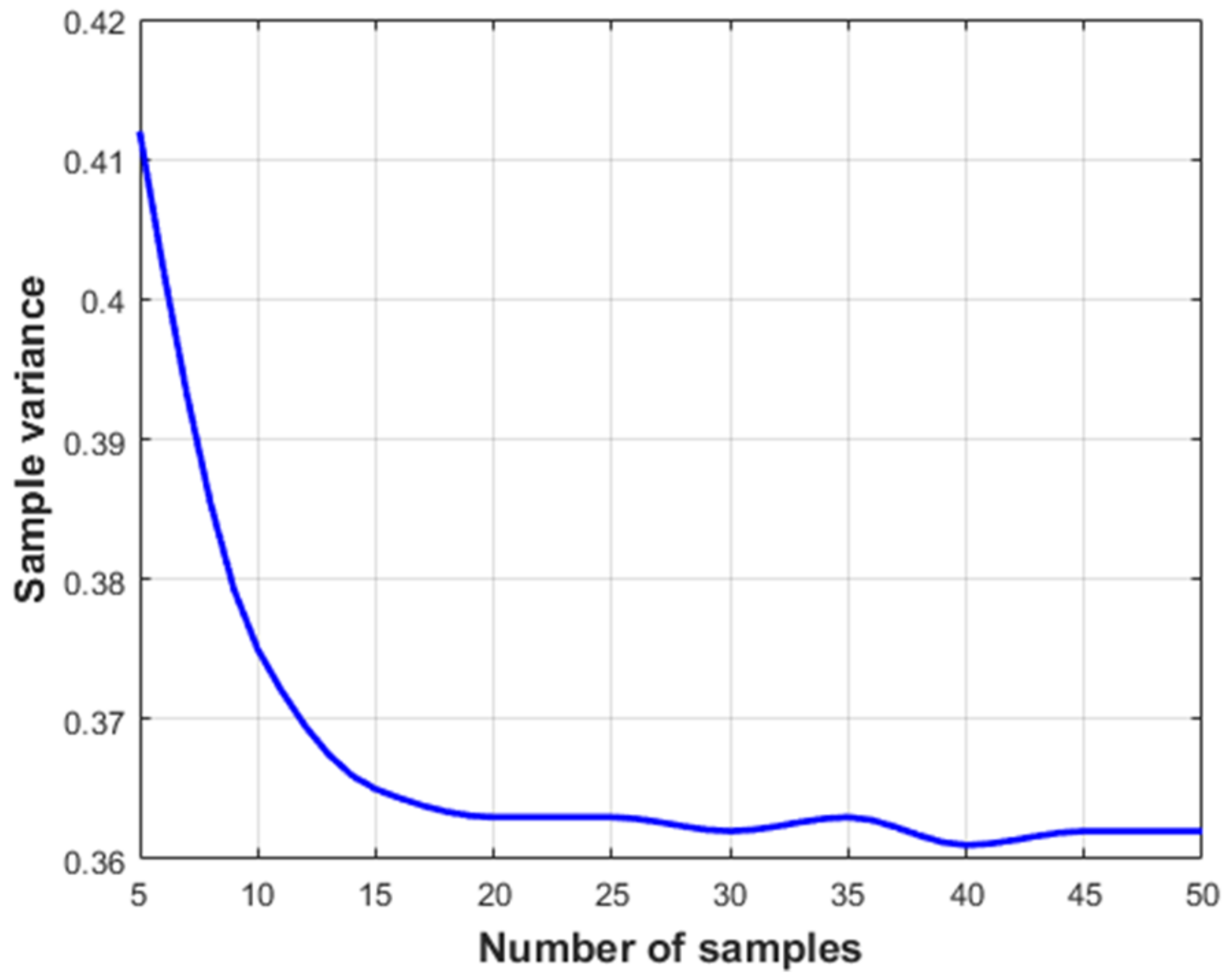
In our model, the number of generated stochastic images might affect the results of uncertainty degree. To illustrate this influence, we ran our method on 10 different images randomly selected from BSD-500 [41], generated multiple stochastic images of each selected image, and calculated the variance between the segmentation result based on the stochastic image sequence. Figure 7 shows that, when the number of stochastic images increases to a certain value, i.e., 20, the standard deviation between segmentation results will not change dramatically. Therefore, we suggest choosing a number with . In addition, the Brownian motion in our method generates stochastic disturbance, being of great help for crossing local saddle points, and contributes to converging to a global optimal value rapidly when optimizing the energy functional. Hence, to verify its effect, we randomly chose 10 different images and segmented each one by solving (14) and (18), respectively. The average value of the energy functional of each image is calculated for different iterations, as shown in Figure 8. The blue one is the convergence curve with the stochastic term, while green is the one without the stochastic term. Obviously, the addition of stochastic term contributes to crossing the saddle points and rapidly converging to an optimized value.
In addition, to verify the effect of uncertainty regularization in the energy functional, i.e., the last term on the right-hand side of (12), we present ablation experiments on the selected 11 images and the entire BSD-500 [41]. We take the method by removing the uncertainty regularization term as baseline, and use the mean of hesitation degree on an image as a measure for uncertainty. The quantities shown in Table 3 suggest that the algorithm with uncertainty regularization could achieve better segmentation performance than the one without uncertainty regularization. Meanwhile, the uncertainty regularization in the energy functional makes the segmentation have low uncertainty.
5. Conclusions
In this paper, we propose a novel stochastic active contour model by designing a novel energy functional of stochastic ACM based on IFS to realize an image segmentation with low uncertainty. In our model, IFS models the uncertainty of human recognition, while stochastic ACM contributes to crossing the saddle points of the energy functional when optimization. The qualitative and quantitative experiments show that the proposed method obtains promising and competitive results on different types of images. The miscellaneous experiments suggest that the proposed method is robust against initial curve, image noise, and blur edges. The experiment on the convergence of Brownian motion verifies the ability of crossing saddle points when optimizing the energy functional. The ablation experiment shows that the uncertainty regularization in the energy functional makes the segmentation have lower uncertainty, which helps to improve the credibility of the segmentation. However, our model still suffers from pretty heavy computation. This is because it needs to perform multiple iterative segmentation on stochastic images. Additionally, intuitionistic fuzzy set could be replaced by more powerful methodologies, e.g., support intuitionistic fuzzy set. The future work might focus on: (1) improving the efficiency by introducing lattice Boltzmann method and parallel programming; and (2) enhancing the model for uncertainty.
Author Contributions
Conceptualization and supervision, B.W.; methodology and software, Y.L.; and validation, J.Z. All authors have read and agreed to the published version of the manuscript.
Funding
This work was partially supported in part by the National Natural Science Foundation of China under Grants 61971331 and 61571347.
Institutional Review Board Statement
Not applicable.
Informed Consent Statement
Not applicable.
Data Availability Statement
The online dataset BSD-500 could be found at https://www2.eecs.berkeley.edu/Research/Projects/CS/vision/bsds/.
Acknowledgments
The authors would like to thank the editor and anonymous reviewers for their critical and constructive comments and suggestions.
Conflicts of Interest
The authors declare no conflict of interest.
Abbreviations
The following abbreviations are used in this manuscript:
| ACM | Active Contour Model |
| LSM | Level Set Method |
| LBF | Local Fitting Model |
| RSF | Region-Scalable Fitting |
| LIF | Local Image Fitting |
| FEBAC | Fuzzy Energy-Based Active Contour |
| PDE | Partial Differential Equation |
| SPDE | Stochastic Partial Differential Equation |
| SDE | Stochastic Differential Equation |
| IFS | Intuitionistic Fuzzy Set |
References
- Liu, C.; Ng, M.K.P.; Zeng, T. Weighted Variational Model for Elective Image Segmentation with Application to Medical Images. Pattern Recognit. 2018, 76, 367–379. [Google Scholar] [CrossRef]
- Zhang, Y.; Su, Y.; Yang, J.; Ponce, J.; Kong, H. When Dijkstra Meets Vanishing Point: A Stereo Vision Approach for Road Detection. IEEE Trans. Image Process. 2018, 27, 2176–2188. [Google Scholar] [CrossRef] [PubMed]
- Liu, C.; Xiao, Y.; Yang, J. A Coastline Detection Method in Polarimetric SAR Images Mixing the Region-Based and Edge-Based Active Contour Models. IEEE Trans. Geosci. Remote Sens. 2017, 55, 3735–3747. [Google Scholar] [CrossRef]
- Kass, M.; Witkin, A.; Terzopoulos, D. Snakes: Active Contour Models. Int. J. Comput. Vis. 1988, 1, 321–331. [Google Scholar] [CrossRef]
- Osher, S.; Sethian, J.A. Fronts Propagating with Curvature-Dependent Speed: Algorithms Based on Hamilton-Jacobi Formulation. J. Comput. Phys. 1988, 79, 12–49. [Google Scholar] [CrossRef] [Green Version]
- Caselles, V.; Kimmel, R.; Sapiro, G. Geodesic Active Contours. Int. J. Comput. Vis. 1997, 22, 61–79. [Google Scholar] [CrossRef]
- Mumford, D.; Shah, J. Optimal Approximations by Piecewise Smooth Functions and Associated Variational Problems. Commun. Pure Appl. Math. 1989, 42, 577–685. [Google Scholar] [CrossRef] [Green Version]
- Chan, T.F.; Vese, L.A. Active Contours without Edges. IEEE Trans. Image Process. 2001, 10, 266–277. [Google Scholar] [CrossRef] [Green Version]
- Tsai, A.; Yezzi, A.; Willsky, A.S. Curve Evolution Implementation of the Mumford-Shah Functional for Image Segmentation, Denoising, Interpolation, and Magnification. IEEE Trans. Image Process. 2001, 10, 1169–1186. [Google Scholar] [CrossRef] [Green Version]
- Li, C.; Kao, C.Y.; Gore, J.C.; Ding, Z. Implicit Active Contours Driven by Local Binary Fitting Energy. In Proceedings of the 2007 IEEE Conference on Computer Vision and Pattern Recognition, Minneapolis, MN, USA, 17–22 June 2007. [Google Scholar]
- Li, C.; Kao, C.Y.; Gore, J.C.; Ding, Z. Minimization of Region-Scalable Fitting Energy for Image Segmentation. IEEE Trans. Image Process. 2008, 17, 1940–1949. [Google Scholar]
- Zhang, K.; Song, H.; Zhang, L. Active Contours Driven by Local Image Fitting Energy. Pattern Recognit. 2010, 43, 1199–1206. [Google Scholar] [CrossRef]
- Gibou, F.; Fedkiw, R. A Fast Hybrid K-Means Level Set Algorithm for Segmentation. In Proceedings of the 2002 4th Annual Hawaii International Conference on Statistics and Mathematics, Hawaii, HI, USA, 28 October–1 November 2002. [Google Scholar]
- Chen, Z.; Qiu, T.; Ruan, S. Fuzzy Adaptive Level Set Algorithm for Brain Tissue Segmentation. In Proceedings of the 2008 9th International Conference on Signal Processing, Beijing, China, 26–29 October 2008. [Google Scholar]
- Krinidis, S.; Chatzis, V. Fuzzy Energy-Based Active Contour. IEEE Trans. Image Process. 2009, 18, 2747–2755. [Google Scholar] [CrossRef] [PubMed]
- Tran, T.T.; Pham, V.T.; Shyu, K.K. Image Segmentation Using Fuzzy Energy-Based Active Contour with Shape Prior. J. Vis. Commun. Image Represent. 2014, 25, 1732–1745. [Google Scholar] [CrossRef]
- Juan, O.; Keriven, R.; Postelnicu, G. Stochastic Motion and the Level Set Method in Computer Vision: Stochastic Active Contours. Int. J. Comput. Vis. 2006, 69, 7–25. [Google Scholar] [CrossRef]
- Mao, W.J.; Chu, J. Stochastic Differential Equations—An Introduction with Applications. IEEE Trans. Autom. Control. 2006, 15, 1731–1732. [Google Scholar]
- Law, Y.N.; Lee, H.K.; Yip, A.M. A Multiresolution Stochastic Level Set Method for Mumford-Shah Image Segmentation. IEEE Trans. Image Process. 2008, 17, 2289–2300. [Google Scholar]
- Dariusz, B.; Katarzyna, J.B. Image Denoising Using Backward Stochastic Differential Equations (Colour Version). Adv. Intell. Syst. Comput. 2017, 659, 185–194. [Google Scholar]
- Hedges, L.O.; Kim, H.A.; Jack, R.L. Stochastic Level-Set Method for Shape Optimisation. J. Comput. Phys. 2017, 348, 82–107. [Google Scholar] [CrossRef] [Green Version]
- Zadeh, L.A. The Concept of a Linguistic Variable and Its Application to Approximate Reasoning—III. Inf. Sci. 1975, 9, 43–80. [Google Scholar] [CrossRef]
- Atanassov, K.T. Intuitionistic Fuzzy Set. Fuzzy Sets Syst. 1986, 20, 87–96. [Google Scholar] [CrossRef]
- Nguyen, X.T. Support-intuitionistic fuzzy set: A new concept for soft computing. Int. J. Intell. Syst. Appl. 2015, 7, 11–16. [Google Scholar] [CrossRef] [Green Version]
- Song, Y.; Wang, X.; Quan, W.; Huang, W. A new approach to construct similarity measure for intuitionistic fuzzy sets. Soft Comput. 2019, 23, 1985–1998. [Google Scholar] [CrossRef]
- Riaz, M.; Çagman, N.; Wali, N.; Mushtaq, A. Certain properties of soft multi-set topology with applications in multi-criteria decision making. Decis. Mak. Appl. Manag. Eng. 2020, 3, 70–96. [Google Scholar] [CrossRef]
- Sahoo, P.K.; Satpathy, P.K.; Patnaik, S. Application of soft computing neural network tools to line congestion study of electrical power systems. Int. J. Inf. Commun. Technol. 2018, 13, 219–226. [Google Scholar] [CrossRef]
- Das, S.; Saha, S. Data mining and soft computing using support vector machine: A survey. Int. J. Comput. Appl. 2013, 77, 40–47. [Google Scholar] [CrossRef]
- Rzheutskaya, S.; Rzheutskiy, A.; Salikhova, R. Applying a genetic algorithm to build a classification tree. In Proceedings of the III International Scientific and Practical Conference, St. Petersburg, Russia, 14–15 March 2020; pp. 1–4. [Google Scholar]
- Zhang, Y.W.; Zhang, W.M.; Peng, K.; Yan, D.C.; Wu, Q.L. A novel edge server selection method based on combined genetic algorithm and simulated annealing algorithm. Automatika 2021, 62, 32–43. [Google Scholar] [CrossRef]
- Niu, S.; Chen, Q.; Sisternes, L.D.; Ji, Z.; Zhou, Z.; Rubin, D.L. Robust Noise Region-Based Active Contour Model Via Local Similarity Factor for Image Segmentation. Pattern Recognit. 2017, 61, 104–119. [Google Scholar] [CrossRef] [Green Version]
- Boncelet, C. Image Noise Models. In The Essential Guide to Image Process; Academic Press: Pittsburgh, PA, USA, 2009. [Google Scholar]
- Peirson, D.; Cawse, P.; Salmon, L.; Cambray, R. Trace Elements in the Atmospheric Environment. Nature 1973, 241, 252–256. [Google Scholar] [CrossRef]
- Tsin, Y.; Ramesh, V.; Kanade, T. Statistical Calibration of CCD Imaging Process. In Proceedings of the 2001 IEEE International Conference on Computer Vision, Vancouver, BC, Canada, 7–14 July 2001. [Google Scholar]
- McCartney, E.J. Optics of the Atmosphere: Scattering by Molecules and Particles. Phys. Today 1977, 30, 76–77. [Google Scholar] [CrossRef]
- Szmidt, E.; Kacprzyk, J. Entropy for Intuitionistic Fuzzy Set. Fuzzy Sets Syst. 2001, 118, 467–477. [Google Scholar] [CrossRef]
- Sugeno, M. Fuzzy Measures and Fuzzy Integral: A Survey. Fuzzy Autom. Decis. Process. 1977, 78, 89–102. [Google Scholar]
- Mao, X. The Truncated Euler–Maruyama Method for Stochastic Differential Equations. J. Comput. Appl. Math. 2015, 290, 370–384. [Google Scholar] [CrossRef] [Green Version]
- Zhang, K.; Zhang, L.; Lam, K.M.; Zhang, D. A Level Set Approach to Image Segmentation with Intensity Inhomogeneity. IEEE Trans. Cybern. 2016, 46, 546–557. [Google Scholar] [CrossRef] [PubMed]
- Li, G.; Zhao, Y.; Zhang, L.; Wang, X.; Zhang, Y.; Guo, F. Entropy-Based Global and Local Weight Adaptive Image Segmentation Models. Tsinghua Sci. Technol. 2019, 25, 149–160. [Google Scholar] [CrossRef]
- Martin, D.; Fowlkes, C.; Tal, D.; Malik, J. A Database of Human Segmented Natural Images and its Application to Evaluating Segmentation Algorithms and Measuring Ecological Statistics. In Proceedings of the 8th International Conference on Computer Vision, Vancouver, BC, Canada, 7–14 July 2001; Volume 2, pp. 416–423. [Google Scholar]
Figure 1.
The block diagram of the proposed stochastic ACM.

Figure 2.
The comparison results on synthetic images. The first column is the images to be segmented, the middle five columns are the segmentation result of the five methods (CV [8], RSF [11], FEBAC [15], RLSF [31], and ours), and the last column is the uncertainty degree.

Figure 3.
The comparison results on medial images. The first column is the images to be segmented, the middle five columns are the segmentation result of the five methods (CV [8], RSF [11], FEBAC [15], RLSF [31], and ours) and the last column is the uncertainty degree generated by our method.

Figure 4.
The comparison results on infrared images. The first column is the images to be segmented, the middle five columns are the segmentation result of the five methods (CV [8], RSF [11], FEBAC [15], RLSF [31], and ours) and the last column is the uncertainty degree generated by our method.

Figure 5.
The comparison results on natural images. The first column is the images to be segmented, the middle five columns are the segmentation result of the five methods (CV [8], RSF [11], FEBAC [15], RLSF [31], and ours) and the last column is the uncertainty degree generated by our method.

Figure 6.
The verification of the robustness against initial curve, noise and blurriness of our method, respectively: (a) Columns 1–4 denote the original image with different initial regions, which are the enclosed by the initial curve, and Column 5 is the final segmentation; (b) the segmentation result on the images with different level noise; and (c) the segmentation results on the images with different smoothness.

Figure 7.
Robustness experiment.

Figure 8.
Convergence with/without Brownian motion.


Table 1.
The quantitative experiments with five methods on the 11 images and BSD-500 [41].
Table 1.
The quantitative experiments with five methods on the 11 images and BSD-500 [41].
| Image | CV | RSF | FEBAC | RLSF | Ours | |||||
|---|---|---|---|---|---|---|---|---|---|---|
| DSC ↑ | JSC ↑ | DSC ↑ | JSC ↑ | DSC ↑ | JSC ↑ | DSC ↑ | JSC ↑ | DSC ↑ | JSC ↑ | |
1.  | 0.634 | 0.618 | 0.989 | 0.961 | 0.637 | 0.611 | 0.991 | 0.973 | 0.993 | 0.972 |
2.  | 0.852 | 0.837 | 0.982 | 0.952 | 0.856 | 0.847 | 0.984 | 0.965 | 0.987 | 0.967 |
3.  | 0.681 | 0.665 | 0.978 | 0.951 | 0.702 | 0.674 | 0.981 | 0.962 | 0.984 | 0.963 |
4.  | 0.783 | 0.766 | 0.974 | 0.944 | 0.825 | 0.798 | 0.976 | 0.958 | 0.978 | 0.956 |
5.  | 0.812 | 0.796 | 0.862 | 0.833 | 0.853 | 0.826 | 0.915 | 0.895 | 0.975 | 0.954 |
6.  | 0.637 | 0.620 | 0.815 | 0.787 | 0.681 | 0.654 | 0.893 | 0.874 | 0.972 | 0.952 |
7.  | 0.785 | 0.768 | 0.542 | 0.512 | 0.802 | 0.774 | 0.887 | 0.866 | 0.965 | 0.943 |
8.  | 0.773 | 0.757 | 0.706 | 0.677 | 0.826 | 0.798 | 0.872 | 0.853 | 0.981 | 0.961 |
9.  | 0.671 | 0.654 | 0.623 | 0.593 | 0.898 | 0.871 | 0.885 | 0.865 | 0.973 | 0.951 |
10.  | 0.814 | 0.798 | 0.587 | 0.560 | 0.925 | 0.897 | 0.902 | 0.884 | 0.987 | 0.967 |
11.  | 0.796 | 0.779 | 0.715 | 0.687 | 0.839 | 0.813 | 0.846 | 0.828 | 0.962 | 0.939 |
| Ave.(1–11) | 0.749 | 0.733 | 0.798 | 0.769 | 0.804 | 0.778 | 0.921 | 0.902 | 0.978 | 0.957 |
| STDEV(1–11) | 0.077 | 0.097 | 0.172 | 0.172 | 0.092 | 0.093 | 0.052 | 0.052 | 0.010 | 0.010 |
| Ave.(BSD-500) | 0.852 | 0.837 | 0.785 | 0.754 | 0.893 | 0.865 | 0.904 | 0.885 | 0.936 | 0.913 |
| STDEV(BSD-500) | 0.071 | 0.075 | 0.079 | 0.081 | 0.064 | 0.061 | 0.062 | 0.065 | 0.057 | 0.059 |
Table 2.
The efficiency experiments with five methods on the 11 images and BSD-500 [41].
Table 2.
The efficiency experiments with five methods on the 11 images and BSD-500 [41].
| Image | CV | RSF | FEBAC | RLSF | Ours |
|---|---|---|---|---|---|
1.  | 3.98 | 4.96 | 3.21 | 15.83 | 5.86 |
2.  | 4.12 | 4.82 | 2.98 | 15.14 | 6.13 |
3.  | 1.85 | 2.71 | 1.59 | 8.78 | 3.31 |
4.  | 1.94 | 2.84 | 1.63 | 8.94 | 3.45 |
5.  | 13.75 | 15.33 | 8.96 | 48.25 | 18.64 |
6.  | 1.83 | 2.57 | 1.52 | 8.37 | 3.26 |
7.  | 16.82 | 18.92 | 11.49 | 53.16 | 22.39 |
8.  | 19.53 | 20.43 | 12.72 | 66.75 | 25.32 |
9.  | 19.45 | 21.38 | 13.02 | 67.19 | 25.58 |
10.  | 18.69 | 21.56 | 12.63 | 66.82 | 25.87 |
11.  | 19.37 | 20.72 | 12.84 | 67.34 | 26.14 |
| Ave.(1–11) | 11.03 | 12.39 | 7.51 | 38.78 | 15.09 |
| STDEV(1–11) | 8.14 | 8.63 | 5.24 | 25.74 | 9.99 |
| Ave.(BSD-500) | 19.37 | 21.25 | 12.86 | 67.24 | 26.13 |
| STDEV(BSD-500) | 0.32 | 0.35 | 0.21 | 0.39 | 0.27 |
Table 3.
The ablation experiments of uncertainty regularization on the 11 images and BSD-500 [41].
Table 3.
The ablation experiments of uncertainty regularization on the 11 images and BSD-500 [41].
| Image | Baseline | Baseline + Uncertainty Reg. | ||||
|---|---|---|---|---|---|---|
| DSC↑ | JSC↑ | HD↓ | DSC↑ | JSC↑ | HD↓ | |
1.  | 0.636 | 0.613 | 0.0048 | 0.993 | 0.972 | 0.0043 |
2.  | 0.859 | 0.848 | 0.0027 | 0.987 | 0.967 | 0.0024 |
3.  | 0.721 | 0.691 | 0.0147 | 0.984 | 0.963 | 0.0124 |
4.  | 0.834 | 0.809 | 0.0128 | 0.978 | 0.956 | 0.0112 |
5.  | 0.875 | 0.846 | 0.0039 | 0.975 | 0.954 | 0.0037 |
6.  | 0.712 | 0.683 | 0.0264 | 0.972 | 0.952 | 0.0244 |
7.  | 0.816 | 0.789 | 0.0038 | 0.965 | 0.943 | 0.0036 |
8.  | 0.845 | 0.819 | 0.0077 | 0.981 | 0.961 | 0.0069 |
9.  | 0.912 | 0.882 | 0.0090 | 0.973 | 0.951 | 0.0083 |
10.  | 0.935 | 0.906 | 0.0108 | 0.987 | 0.967 | 0.0101 |
11.  | 0.852 | 0.825 | 0.0102 | 0.962 | 0.939 | 0.0095 |
| Ave.(1–11) | 0.818 | 0.792 | 0.0097 | 0.978 | 0.957 | 0.0088 |
| STDEV(1–11) | 0.019 | 0.091 | 0.0068 | 0.010 | 0.010 | 0.0062 |
| Ave.(BSD-500) | 0.899 | 0.874 | 0.0094 | 0.936 | 0.913 | 0.0087 |
| STDEV(BSD-500) | 0.062 | 0.063 | 0.0016 | 0.057 | 0.059 | 0.0014 |
Publisher’s Note: MDPI stays neutral with regard to jurisdictional claims in published maps and institutional affiliations. |
© 2021 by the authors. Licensee MDPI, Basel, Switzerland. This article is an open access article distributed under the terms and conditions of the Creative Commons Attribution (CC BY) license (http://creativecommons.org/licenses/by/4.0/).
Share and Cite
MDPI and ACS Style
Wang, B.; Li, Y.; Zhang, J. An Intuitionistic Fuzzy Set Driven Stochastic Active Contour Model with Uncertainty Analysis. Mathematics 2021, 9, 301. https://doi.org/10.3390/math9040301
AMA Style
Wang B, Li Y, Zhang J. An Intuitionistic Fuzzy Set Driven Stochastic Active Contour Model with Uncertainty Analysis. Mathematics. 2021; 9(4):301. https://doi.org/10.3390/math9040301
Chicago/Turabian StyleWang, Bin, Yaoqing Li, and Jianlong Zhang. 2021. "An Intuitionistic Fuzzy Set Driven Stochastic Active Contour Model with Uncertainty Analysis" Mathematics 9, no. 4: 301. https://doi.org/10.3390/math9040301
Note that from the first issue of 2016, this journal uses article numbers instead of page numbers. See further details here.