Inverse Problem of Recovering the Initial Condition for a Nonlinear Equation of the Reaction–Diffusion–Advection Type by Data Given on the Position of a Reaction Front with a Time Delay

Abstract

In this paper, approaches to the numerical recovering of the initial condition in the inverse problem for a nonlinear singularly perturbed reaction–diffusion–advection equation are considered. The feature of the formulation of the inverse problem is the use of additional information about the value of the solution of the equation at the known position of a reaction front, measured experimentally with a delay relative to the initial moment of time. In this case, for the numerical solution of the inverse problem, the gradient method of minimizing the cost functional is applied. In the case when only the position of the reaction front is known, the method of deep machine learning is applied. Numerical experiments demonstrated the possibility of solving such kinds of considered inverse problems.

1. Introduction

This paper discusses the inverse problem of numerical recovering of the initial condition for a nonlinear singularly perturbed reaction–diffusion–advection equation with data on the position of a reaction front, measured in an experiment with a delay relative to the initial time. Problems for equations of this type arise in gas dynamics [1], chemical kinetics [2,3,4,5,6], nonlinear wave theory [7], biophysics [8,9,10,11,12], medicine [13,14,15,16], ecology [17,18,19] and other fields of science [20]. A feature of this type of problem is the presence of multi-scale processes. Mathematical formulations of these problems are described by nonlinear parabolic equations with a small parameter at the highest derivative. Therefore, solutions of these problems are able to contain narrow boundary and/or interior layers (stationary and/or moving fronts).

In the formulations of inverse problems for partial differential equations additional information about the solution on a part of the boundary is often used (see, for example, [21,22,23,24,25,26,27,28,29,30]). For example, in formulation of so-called inverse backward problem (or retrospective inverse problems) it is required to find a solution at the initial time from a known solution at the final time [31,32,33]. This type of problem is ill-posed [24,34,35]. For solving retrospective inverse problems for parabolic equations the following methods have been used: quasi-reversibility [36,37], optimal filtering [38], boundary element [39], mollification [40], group preserving [41], operator-splitting [42], Fourier regularization [43,44], modified Tikhonov regularization [45], sequential function specification [31], and collocation [46].

However, one of the possible formulations of the inverse problem for determining the initial condition is a statement with additional information about the dynamics of the reaction front movement, if it is available for experimental observation (position of the shock wave front, reaction or combustion front, etc.). Moreover, under certain conditions, observation of the reaction front can be started only with a certain time delay. This may be due to both experimental limitations and the fact that at the initial moment of time there is no reaction front at all. The latter case is possible in a situation in which the reaction front is formed (and, therefore, can be observed) only some time after the start of the experiment.

The difference between the formulations of inverse problems of recovering the initial condition with the data at the final time moment and with the data on the position of the reaction front measured with a time delay are shown in Figure 1.

The formulation of the inverse problem of recovering the initial condition considered in this paper is quite new.

In the proposed formulation, it is impossible to extract a priori information about the solution of the inverse problem using the methods of asymptotic analysis [2,47], because the data of the inverse problem do not contain information about the reaction front at all times, including the initial time. This significantly distinguishes this work from the previous works of the authors [48,49,50]. Now we consider the formulation of the inverse problem, in which the requirement for the presence of an experimentally distinguishable reaction front at the initial moment of time is not required.

The structure of this work is as follows. Section 2 contains (1) the formulation of the inverse problem of recovering the initial condition for a nonlinear singularly perturbed reaction–diffusion–advection equation based on additional information about the value of the solution of the equation at the known position of the reaction front, measured experimentally with a delay relative to the initial time and (2) a method for solving it, based on minimizing the target functional by the gradient method. This section also demonstrates the results of numerical experiments, from which it is possible to draw conclusions about the capabilities of the proposed method. Section 3 discusses a deep machine learning method for solving the inverse problem of restoring the initial condition from additional information about the position of the reaction front without knowing the solution to the equation on this front, i.e., the inverse problem is solved with less additional information.

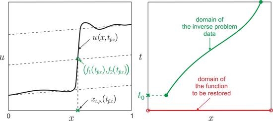
2. Statement of the Inverse Problem and a Gradient Method of Its Solution

Let us consider the following direct problem for a nonlinear singularly perturbed Burgers-type equation [51]:

$$\left\{\begin{array}{c}\epsilon \frac{{\partial }^{2}u}{\partial x^2}-\frac{\partial u}{\partial t}=-u\frac{\partial u}{\partial x}+u,x\in (0,1),t\in (0,T],\hfill \\ u(0,t)=u_{left}\left(t\right),u(1,t)=u_{right}\left(t\right),t\in [0,T],\hfill \\ u(x,0)=q\left(x\right),x\in (0,1),\hfill \end{array}\right.$$

(1)

where $0<\epsilon \ll 1$ is a small parameter, and functions $q\left(x\right)$, $u_{left}\left(t\right)$ and $u_{right}\left(t\right)$ are sufficiently smooth.

In some situations it is possible that a moving front of the reaction starts forming from a certain moment of time $t_0\ge 0$. In this case, the solution of the problem (1) will approach over time to two different functions ${\phi }^l\left(x\right)$ and ${\phi }^r\left(x\right)$ to the left and right of some point $x_{t.p.}\left(t\right)$, and in a small (of the order of $\epsilon |ln\epsilon |$) neighborhood of this point, a narrow internal transition layer will be observed (see Figure 2) [2,47]. The point $x_{t.p.}\left(t\right)$ we will call as “transition point” (“t.p.”).

Note that it is known from [50] that for the problem (1) the expressions for ${\phi }^l\left(x\right)$ and ${\phi }^r\left(x\right)$ can be written out explicitly: ${\phi }^l\left(x\right)=u_{left}\left(t\right)+x$ and ${\phi }^r\left(x\right)=u_{right}\left(t\right)+x-1$.

The function $x=x_{t.p.}\left(t\right)$, which describes the position of the reaction front, can be found as a solution to, for example, the following functional equation [50]:

$$u(x,t)=\phi \left(x\right)\equiv {\displaystyle \frac{1}{2}}\left({\phi }^l\left(x\right)+{\phi }^r\left(x\right)\right),t\in [t_0,T].$$

Thus, we can match the conditions (parameters) of the problem (1), which has a solution like a moving front on the time segment $[t_0,T]\subseteq [0,T]$, the position of this reaction front $x_{t.p.}\left(t\right)\equiv f_1\left(t\right)$ at any time $t\in [t_0,T]$, as well as the value of the function $u\left(x_{t.p.}\left(t\right),t\right) \equiv f_2\left(t\right)$ (see Figure 1).

The inverse problem is to determine the initial condition $q_{{\delta }_1,{\delta }_2}\left(x\right)$, $x\in (0,1)$, from some known additional information about the position of the reaction front and the value of the function u at this front

$$x_{t.p.}\left(t\right)={f_1}_{{\delta }_1}\left(t\right),u\left(x_{t.p.}\left(t\right),t\right)={f_2}_{{\delta }_2}\left(t\right),t\in [t_0,T]\subseteq [0,T],$$

(2)

experimentally observed with errors ${\delta }_1$ and ${\delta }_2$:

$$\parallel f_1-{f_1}_{{\delta }_1}{\parallel }_{L_2}\le {\delta }_1,{\parallel f_2-{f_2}_{{\delta }_2}\parallel }_{L_2}\le {\delta }_2.$$

Remark 1.

Note that the features of solving the retrospective inverse problem (an inverse backward problem) for (1) were considered in [50].

In operator form, this statement can be rewritten as

$$A\left(q_{{\delta }_1,{\delta }_2}\right)=\left\{{f_1}_{{\delta }_1},{f_2}_{{\delta }_2}\right\}.$$

(3)

here

$$\begin{array}{cc}\hfill & A=\{A_1,A_2\},A_1:q_{{\delta }_1,{\delta }_2}\left(x\right)\to x_{t.p.}\left(t\right)={f_1}_{{\delta }_1}\left(t\right),\hfill \\ \hfill & A_2:q_{{\delta }_1,{\delta }_2}\left(x\right)\to u\left(x_{t.p.}\left(t\right),t\right)={f_2}_{{\delta }_2}\left(t\right).\hfill \end{array}$$

Let us reduce the inverse problem (3) to minimization of the cost functional

$$J\left[q\right]=\parallel A_2\left(q\right)-{f_2}_{{\delta }_2}{\parallel }_{L_2(t_0,T)}^2\to \underset{q}{min}$$

by the gradient method [24,25,52,53]. Thus, the solution of the inverse problem (1)–(2) can be found as an element $q_{{\delta }_1,{\delta }_2}$, realizing the minimum of the functional

$$J\left[q\right]=\underset{t_0}{\overset{T}{\int }}{\left(u\left({f_1}_{{\delta }_1}\left(t\right),t;q\right)-{f_2}_{{\delta }_2}\left(t\right)\right)}^{2}dt,$$

(4)

where $u(x,t;q)$ is the solution of the direct problem (1) for a given function $q\left(x\right)$.

The algorithm of gradient method for numerical solving of the inverse problem (1)–(2) is formulated as follows.

• Set $s:=0$ and $q^{\left(0\right)}\left(x\right)$ as an initial guess.
• Find the solution $u^{\left(s\right)}(x,t)$ of the direct problem:

  $$\left\{\begin{array}{c}\epsilon \frac{{\partial }^2{u}^{\left(s\right)}}{\partial x^2}-\frac{\partial u^{\left(s\right)}}{\partial t}=-u^{\left(s\right)}\frac{\partial u^{\left(s\right)}}{\partial x}+u^{\left(s\right)},x\in (0,1),t\in (0,T],\hfill \\ u^{\left(s\right)}(0,t)=u_{left}\left(t\right),u^{\left(s\right)}(1,t)=u_{right}\left(t\right),t\in [0,T],\hfill \\ u^{\left(s\right)}(x,0)=q^{\left(s\right)}\left(x\right),x\in (0,1).\hfill \end{array}\right.$$
• Find the solution ${\psi }^{\left(s\right)}(x,t)$ of the adjoint problem:

  $$\left\{\begin{array}{c}\epsilon \frac{{\partial }^2{\psi }^{\left(s\right)}}{\partial x^2}+\frac{\partial {\psi }^{\left(s\right)}}{\partial t}=u^{\left(s\right)}\frac{\partial {\psi }^{\left(s\right)}}{\partial x}+{\psi }^{\left(s\right)}+\hfill \\ +2\theta (t-t_0)\delta (x-{f_1}_{{\delta }_1}\left(t\right))(u^{\left(s\right)}(x,t)-{f_2}_{{\delta }_2}\left(t\right)),x\in (0,1),t\in [0,T),\hfill \\ {\psi }^{\left(s\right)}(0,t)=0,{\psi }^{\left(s\right)}(1,t)=0,t\in [0,T],\hfill \\ {\psi }^{\left(s\right)}(x,T)=0,x\in (0,1).\hfill \end{array}\right.$$

  (5)
  Here $\delta \left(x\right)$ is the Dirac delta function., $\theta \left(t\right)$ is the Heaviside step function.
• Find the gradient of the functional (4):

  $$J^{\prime }\left[q^{\left(s\right)}\right]\left(x\right)=-{\psi }^{\left(s\right)}(x,0).$$
• Find an approximate solution at the next step of the iteration:

  $$q^{(s+1)}\left(x\right)=q^{\left(s\right)}\left(x\right)-{\beta }_s{J}^{\prime }\left[q^{\left(s\right)}\right]\left(x\right),$$

  (6)

  where ${\beta }_s$ is the descent parameter.
• Check a condition for stopping the iterative process. If it is satisfied, we put $q^{inv}\left(x\right):=q^{(s+1)}\left(x\right)$ as a solution of the inverse problem. Otherwise, set $s:=s+1$ and go to step 2.

  (a)

  In the case of experimental data measured with errors ${\delta }_1$ and ${\delta }_2$, the stopping criterion is

  $$\begin{array}{cc}\hfill & \underset{t_0}{\overset{T}{\int }}\left[{\left(x_{t.p.}\left(t;q^{(s+1)}\right)-{f_1}_{{\delta }_1}\left(t\right)\right)}^{2}dt+{\left(u\left({f_1}_{{\delta }_1}\left(t\right),t;q^{(s+1)}\right)-{f_2}_{{\delta }_2}\left(t\right)\right)}^2\right]dt\le \hfill \\ \hfill & \le {\delta }_1^2+{\delta }_2^2.\hfill \end{array}$$

  Here $x_{t.p.}\left(t;q\right)$ is the position of the reaction front determined by the direct problem (1) for a given function $q\left(x\right)$.

  (b)

  In the case of exact input data, the iterative process stops when $J\left[q^{\left(s\right)}\right]$ is less than the error of the finite-difference approximation.

Remark 2.

Note that the iteration number s of the gradient method is a regularization parameter [25,52,53].

Remark 3.

The convergence of the gradient method (6) for inverse and ill-posed problems was considered in [54,55,56].

Examples of Numerical Calculations

Let us consider the efficiency of the above-proposed algorithm by the example of solving the inverse problem (1)–(2) for the following model set of parameters:

$$\begin{array}{cc}\hfill & q\left(x\right)\equiv q^{model}\left(x\right)=x+1+2sin\left(5\pi x\right),\hfill \\ \hfill & \epsilon ={10}^{-1.5},T=0.7,t_0=T/100,\hfill \\ \hfill & u_{left}\left(t\right)=6e^{-100t}-5,u_{right}\left(t\right)=2.\hfill \end{array}$$

(7)

Figure 3 shows the solutions to the direct problem (1). The process of convergence of the solution to the functions ${\phi }^l\left(x\right)$ and ${\phi }^r\left(x\right)$ is clearly observed to the left and right of the point $x_{t.p.}\left(t\right)$, in the vicinity of which the front of reaction is located.

Figure 4 shows the model functions $f_1\left(t\right)$, $f_2\left(t\right)$ and the result of restoring the function $q\left(x\right)$ from the simulated data ${f_1}_{{\delta }_1}\left(t\right)$ and ${f_2}_{{\delta }_2}\left(t\right)$ specified with errors. For simulating input data, solving the direct problem (1) (step 2 of the algorithm) and the adjoint problem (5) (step 3 of the algorithm) a stiff method of lines, SMOL [57], which allows one to reduce the system of partial differential equations to a system of ordinary differential equations. The resulting systems of differential equations were solved using a single-stage Rosenbrock scheme with a complex coefficient, CROS1 [58,59]. A detailed description of the numerical solving of such problems can be found, for example, in [48]. To simulate the input data, we used grids with $N=1000$ and $M=1000$ intervals for the spatial and temporal variables, respectively. The descent parameter was set as ${\beta }_s={10}^{-4}$. The function $q^{\left(0\right)}\left(x\right)\equiv 0$ was used as an initial guess (approximation). When solving the adjoint problem (5) (step 3 of the algorithm), the following formula was used to approximate the $\delta$–function [60]:

$$\delta \left(x\right)=\left\{\begin{array}{ccc}{\displaystyle \frac{2}{\omega }}\left(1-\left|{\displaystyle \frac{x}{\omega }}\right|-4|{\displaystyle \frac{x}{\omega }}{|}^2+4|{\displaystyle \frac{x}{\omega }}{|}^3\right),\hfill & \hfill & \left|{\displaystyle \frac{x}{\omega }}\right|\le {\displaystyle \frac{1}{2}},\hfill \\ {\displaystyle \frac{2}{\omega }}\left(1-{\displaystyle \frac{11}{3}}\left|{\displaystyle \frac{x}{\omega }}\right|+4|{\displaystyle \frac{x}{\omega }}{|}^2-{\displaystyle \frac{4}{3}}|{\displaystyle \frac{x}{\omega }}{|}^3\right),\hfill & \hfill & {\displaystyle \frac{1}{2}}<\left|{\displaystyle \frac{x}{\omega }}\right|\le 1,\hfill \\ 0,\hfill & \hfill & \left|{\displaystyle \frac{x}{\omega }}\right|>1,\hfill \end{array}\right.$$

where the support size of the discrete delta function: $\omega ={10}^{-2}$. To calculate the integral (step 4 of the algorithm), the trapezoid rule was used.

It is known [35] that when restoring a function of one argument from the results of measuring a function/functions of another argument, the amount of information used matters. In other words, the quality of reconstruction of the required function $q\left(x\right)$ depends not only on the error levels ${\delta }_1$ and ${\delta }_2$ of the input data set, but also from the start time of the observation $t_0$ and the final moment of time.

Let us investigate the quality of reconstruction of the desired function $q\left(x\right)$ depending on the amount of input data. To do this, for different values of $t_0$ (the other parameters in the model example (7) remain unchanged), we find an approximate solution to the inverse problem $q^{inv}\left(x\right)$. From the dependence $\parallel q^{inv}-q^{model}{\parallel }_{L_2}$ on $t_0$ (see Figure 5) we can conclude that the quality of restoration strongly depends on the value $t_0$: the smaller it is, the more accurately the unknown function is restored. The value of T is of secondary importance if it exceeds the time required for the complete formation of a solution of the moving front type (solutions close to the functions ${\phi }^l\left(x\right)$ and ${\phi }^r\left(x\right)$ to the left and right of the point $x_{t.p.}\left(t\right)\equiv f_1\left(t\right)$) [2,47].

Now, let us investigate the stability of the solution to the inverse problem depending on the error level of the input data ${\delta }_1$ and ${\delta }_2$. To do this, for different values of $t_0$ and different values of ${\delta }_1$ and ${\delta }_2$, we find an approximate solution to the inverse problem $q^{inv}\left(x\right)$ (the other parameters in the model example (7) remain unchanged). Figure 6 shows the dependence of $\parallel q^{inv}-q^{model}{\parallel }_{L_2}$ on the input data error level “$\delta$” $=\sqrt{{\left({\delta }_1/<{\parallel {f_1}_{{\delta }_1}\left(t\right)\parallel }_{L_2}>\right)}^2+{\left({\delta }_2/<{\parallel {f_2}_{{\delta }_2}\left(t\right)\parallel }_{L_2}>\right)}^2}·100\%$ expressed as a percentage, where $<cdot>$ means averaging over the set of experiments for the same ${\delta }_{1,2}$. It can be seen that as $\delta$ decreases, the accuracy of recovering the function $q^{inv}\left(x\right)$ increases. Moreover, smaller values of $t_0$ lead to a more accurate reconstruction of the desired function $q\left(x\right)$.

3. Deep Machine Learning Method

When applying the gradient method for minimizing the target functional described in the previous section, additional information is used about two functions $f_1\left(t\right)$ and $f_2\left(t\right)$. Thus, an inverse problem arises of recovering one function of a spatial variable from two time-dependent functions.

From an experimental point of view, this imposes practical limitations on the applicability of the considered approach. Obviously, it is easier to obtain experimental information only about the function $f_1\left(t\right)$, which determines the position of the front, than about the second additional function $f_2\left(t\right)$.

Thus, the following question arises. Is it possible to develop a method that allows solving problems of this type in the following formulation: it is necessary to restore one function of one spatial argument from the results of measurements of one function of one time variable? This question can be solved by applying deep machine learning methods [61,62,63], the use of which in solving the problem under consideration seems quite effective. This is due to the fact that a neural network [61] is a multiparametric nonlinear function that can approximate a real physical law that sets the correspondence between the position of the reaction front and the initial condition that needs to be determined. Moreover, the trained neural network in the case of the problem under consideration allows obtaining good results, since we have an explicit relationship between the function being restored and the input data, determined by the well-known mathematical formulation of the direct problem.

In one of the examples considered in [61], the possibility of recovering the constant coefficient was demonstrated when solving the inverse problem for a nonlinear partial differential equation with data on a part of the boundary. In this paper, we consider restoring the initial condition as a function of the spatial variable and written as a sum of three series in basis functions, from the data on a certain curve inside the considered region. For the numerical implementation, we use MLP [62] and LSTM [63] neural networks.

It should be noted that the approach considered below is effective only for the case when inverse problems of the considered class must be solved many times. This is due to the fact that training a neural network for arbitrary basis functions (and for arbitrary boundary conditions) requires a significant amount of time, but it is performed only once. Then, for a specific input data, the result is obtained in negligible amount of time.

Examples of Numerical Calculations

Let us first describe the generation of a dataset for training neural networks. To train MLP and LSTM neural networks, we use a synthetic dataset obtained by solving a direct problem. For each previously generated set of grid values $q\left(x_n\right)$, $x_n\in (0,1)$, $n=\overline{1,N-1}$, of the function $q\left(x\right)$, we solve the direct problem (1) and get a set of grid values ${f_1}_{{\delta }_1}\left(t_m\right)$, $t_m\in [t_0,T]$, $m=\overline{0,M}$, of functions ${f_1}_{{\delta }_1}\left(t\right)$.

To generate a set of grid values (dataset) of the function $q\left(x\right)$, we will use the parameterized basis function $q^{base}\left(x\right)$ of the following form:

$$q^{base}(x;{\left\{p_i\right\}}_{j=0}^P,{\left\{s_j\right\}}_{j=1}^{F_s};{\left\{c_j\right\}}_{j=1}^{F_c})=\sum _{j=0}^P{p}_j{x}^j+\sum _{j=1}^{F_s}{s}_{j}sin\left(j\pi x\right)+\sum _{j=1}^{F_c}{c}_{j}cos\left(j\pi x\right).$$

Note that such choice of the basis function (including the specific values of P, $F_s$, and $F_c$) is heuristic. Another choice of this function can either improve the quality of the solution or degrade it.

Specific sample $\widehat{q}$:

$$\widehat{q}\equiv q^{base}\left(x;{\left\{{\widehat{p}}_i\right\}}_{j=0}^P,{\left\{{\widehat{s}}_j\right\}}_{j=1}^{F_s};{\left\{{\widehat{c}}_j\right\}}_{j=1}^{F_c}\right)$$

we will generate for random coefficients ${\widehat{p}}_j\sim \mathcal{N}(p_j,p_j^2+1)$, ${\widehat{s}}_j\sim \mathcal{N}(s_j,s_j^2+1)$ and ${\widehat{c}}_j\sim \mathcal{N}(c_j,c_j^2+1)$, where $\mathcal{N}(\mu ,{\sigma }^2)$ is normal distribution with expectation $\mu$ and standard deviation $\sigma$.

For numerical experiments $P=1$, $F_s=5$, and $F_c=2$ were chosen with the factors $\{p_0,p_1\}=\{1,1\}$, $\{s_1,s_2,s_3,s_4,s_5\}=\{0,0,0,0,5\}$ and $\{c_1,c_2\}=\{0,2\}$. An arbitrary set of functions $\widehat{q}\left(x\right)$ for these parameters is shown in Figure 7.

To solve the inverse problem under consideration, we used a neural network consisting of a bundle of LSTM + MLP. The LSTM + MLP network consists of a bidirectional LSTM neural network with a hidden state size of 200 and an MLP neural network with two hidden layers of size 400 and nonlinearity ReLU [64,65]. The LSTM neural network is used to transform the sequence ${f_1}_{{\delta }_1}\left(t_m\right)$, $t_m\in [t_0,T]$, $m=\overline{0,M}$, into a hidden state for subsequent transfer to MLP.

The result of restoring the function $q^{inv}\left(x\right)$ for the model example (7) after training the neural network can be seen in Figure 8. Note that the result of the reconstruction of the unknown function turned out to be much more accurate than the approach considered in the previous section. This is primarily due to the fact that for training the neural network we chose a quite good dataset that is close enough to the solution of the problem. In the case of restoring a function, which does not lie in this dataset (this is equivalent to the case of using “bad” dataset) recovery results become worse (see Figure 9). However, this does not limit the generality, since our main goal is to demonstrate the possibility in principle of using deep machine learning to solve the inverse problem under consideration with limited experimental data.

4. Discussion

• The question of the theoretical justification of the uniqueness and stability of the solution of the considered inverse problem remains open. This may be the subject for a separate work. In this article, we limited ourselves to testing the effectiveness of the proposed approach using numerical experiments.
• When constructing the objective functional, it is possible to use additional smoothing terms (for example, in the form of Tikhonov’s functional [53]). We have limited ourselves to considering the cost functional that determines the least squares method, since its use has already given rather good results.
• Applying deep machine learning, we aimed to demonstrate the fundamental possibility of solving problems of the considered type with limited experimental data using this method. In this regard, we used a fairly good dataset to train the neural network. The question of choosing the optimal neural network configuration remains open. This issue is of significant interest and may be the topic of a separate work.
• The methods of asymptotic analysis were used only to determine the function $x_{t.p.}\left(t\right)$ in the formulation of the direct problem. However, other equivalent ways of defining this function are possible that will not affect the quality of the recovered solution.

5. Conclusions

We considered the inverse problem of recovering the initial condition for a nonlinear singularly perturbed reaction–diffusion–advection equation based on additional information about the value of the solution to the equation at the known position of the reaction front, measured experimentally with a delay relative to the initial time. The inverse problem is reduced to minimization of the cost functional by the gradient method. Numerical calculations have demonstrated the good potential of the proposed approach. For the inverse problem of recovering the initial condition from additional information about the position of the reaction front without knowing the solution to the equation on this front, the method of deep machine learning is applied. Numerical experiments have demonstrated that the cost of efficiency of this method is the ability to construct a good dataset for training the neural network. The possibility of solving such problems by this method is demonstrated.

References

1. Danilov, V.; Maslov, V.; Volosov, K. Mathematical Modelling of Heat and Mass Transfer Processes; Kluwer: Dordrecht, The Netherlands, 1995. [Google Scholar]
2. Butuzov, V.; Vasil’eva, A. Singularly perturbed problems with boundary and interior layers: Theory and applications. Adv. Chem. Phys. 1997, 97, 47–179. [Google Scholar]
3. Liu, Z.; Liu, Q.; Lin, H.C.; Schwartz, C.; Lee, Y.H.; Wang, T. Three-dimensional variational assimilation of MODIS aerosol optical depth: Implementation and application to a dust storm over East Asia. J. Geophys. Res. Atmos. 2010, 116. [Google Scholar] [CrossRef] [Green Version]
4. Egger, H.; Fellner, K.; Pietschmann, J.F.; Tang, B.Q. Analysis and numerical solution of coupled volume-surface reaction-diffusion systems with application to cell biology. Appl. Math. Comput. 2018, 336, 351–367. [Google Scholar] [CrossRef] [Green Version]
5. Yaparova, N. Method for determining particle growth dynamics in a two-component alloy. Steel Transl. 2020, 50, 95–99. [Google Scholar] [CrossRef]
6. Wu, X.; Ni, M. Existence and stability of periodic contrast structure in reaction-advection-diffusion equation with discontinuous reactive and convective terms. Commun. Nonlinear Sci. Numer. Simul. 2020, 91, 105457. [Google Scholar] [CrossRef]
7. Volpert, A.; Volpert, V.; Volpert, V. Traveling Wave Solutions of Parabolic Systems; American Mathematical Society: Providence, RI, USA, 2000. [Google Scholar]
8. Meinhardt, H. Models of Biological Pattern Formation; Academic Press: London, UK, 1982. [Google Scholar]
9. FitzHugh, R. Impulses and physiological states in theoretical model of nerve membrane. Biophys. J. 1961, 1, 445–466. [Google Scholar] [CrossRef] [Green Version]
10. Murray, J. Mathematical Biology. I. An Introduction; Springer: New York, NY, USA, 2002. [Google Scholar] [CrossRef]
11. Egger, H.; Pietschmann, J.F.; Schlottbom, M. Identification of nonlinear heat conduction laws. J. Inverse Ill-Posed Probl. 2015, 23, 429–437. [Google Scholar] [CrossRef] [Green Version]
12. Gholami, A.; Mang, A.; Biros, G. An inverse problem formulation for parameter estimation of a reaction-diffusion model of low grade gliomas. J. Math. Biol. 2016, 72, 409–433. [Google Scholar] [CrossRef] [Green Version]
13. Aliev, R.; Panfilov, A.V. A simple two-variable model of cardiac excitation. Chaos Solitons Fractals 1996, 7, 293–301. [Google Scholar] [CrossRef]
14. Generalov, E.; Levashova, N.; Sidorova, A.; Chumankov, P.; Yakovenko, L. An autowave model of the bifurcation behavior of transformed cells in response to polysaccharide. Biophysics 2017, 62, 876–881. [Google Scholar] [CrossRef]
15. Mang, A.; Gholami, A.; Davatzikos, C.; Biros, G. PDE-constrained optimization in medical image analysis. Optim. Eng. 2018, 19, 765–812. [Google Scholar] [CrossRef] [Green Version]
16. Kabanikhin, S.I.; Shishlenin, M.A. Recovering a Time-Dependent Diffusion Coefficient from Nonlocal Data. Numer. Anal. Appl. 2018, 11, 38–44. [Google Scholar]
17. Mamkin, V.; Kurbatova, J.; Avilov, V.; Mukhartova, Y.; Krupenko, A.; Ivanov, D.; Levashova, N.; Olchev, A. Changes in net ecosystem exchange of CO2, latent and sensible heat fluxes in a recently clear-cut spruce forest in western Russia: Results from an experimental and modeling analysis. Environ. Res. Lett. 2016, 11, 125012. [Google Scholar] [CrossRef]
18. Levashova, N.; Muhartova, J.; Olchev, A. Two approaches to describe the turbulent exchange within the atmospheric surface layer. Math. Model. Comput. Simul. 2017, 9, 697. [Google Scholar] [CrossRef]
19. Levashova, N.; Sidorova, A.; Semina, A.; Ni, M. A spatio-temporal autowave model of shanghai territory development. Sustainability 2019, 11, 3658. [Google Scholar] [CrossRef] [Green Version]
20. Kadalbajoo, M.; Gupta, V. A brief survey on numerical methods for solving singularly perturbed problems. Appl. Math. Comput. 2010, 217, 3641–3716. [Google Scholar] [CrossRef]
21. Cannon, J.; DuChateau, P. An Inverse problem for a nonlinear diffusion equation. SIAM J. Appl. Math. 1980, 39, 272–289. [Google Scholar] [CrossRef]
22. DuChateau, P.; Rundell, W. Unicity in an inverse problem for an unknown reaction term in a reaction-diffusion equation. J. Differ. Equ. 1985, 59, 155–164. [Google Scholar] [CrossRef] [Green Version]
23. Pilant, M.; Rundell, W. An inverse problem for a nonlinear parabolic equation. Commun. Partial. Differ. Equ. 1986, 11, 445–457. [Google Scholar] [CrossRef]
24. Kabanikhin, S. Definitions and examples of inverse and ill-posed problems. J. Inverse Ill-Posed Probl. 2008, 16, 317–357. [Google Scholar] [CrossRef]
25. Kabanikhin, S. Inverse and Ill-posed Problems Theory and Applications; de Gruyter: Berlin, Germany, 2011. [Google Scholar]
26. Jin, B.; Rundell, W. A tutorial on inverse problems for anomalous diffusion processes. Inverse Probl. 2015, 31, 035003. [Google Scholar] [CrossRef] [Green Version]
27. Belonosov, A.; Shishlenin, M. Regularization methods of the continuation problem for the parabolic equation. Lect. Notes Comput. Sci. 2017, 10187, 220–226. [Google Scholar]
28. Kaltenbacher, B.; Rundell, W. On the identification of a nonlinear term in a reaction-diffusion equation. Inverse Probl. 2019, 35, 115007. [Google Scholar] [CrossRef] [Green Version]
29. Belonosov, A.; Shishlenin, M.; Klyuchinskiy, D. A comparative analysis of numerical methods of solving the continuation problem for 1D parabolic equation with the data given on the part of the boundary. Adv. Comput. Math. 2019, 45, 735–755. [Google Scholar] [CrossRef]
30. Kaltenbacher, B.; Rundell, W. The inverse problem of reconstructing reaction-diffusion systems. Inverse Probl. 2020, 36, 065011. [Google Scholar] [CrossRef]
31. Beck, J.V.; Blackwell, B.; Claire, C.R.S.J. Inverse Heat Conduction: Ill-Posed Problems; Wiley: New York, NY, USA, 1985. [Google Scholar]
32. Alifanov, O.M. Inverse Heat Transfer Problems; International Series in Heat and Mass Transfer; Springer: Berlin/Heidelberg, Germany, 1994. [Google Scholar]
33. Ismail-Zadeh, A.; Korotkii, A.; Schubert, G.; Tsepelev, I. Numerical techniques for solving the inverse retrospective problem of thermal evolution of the Earth interior. Comput. Struct. 2009, 87, 802–811. [Google Scholar] [CrossRef]
34. Lavrent’ev, M.; Romanov, V.; Shishatskij, S. Ill-Posed Problems of Mathematical Physics and Analysis, Translations of Mathematical Monographs; Schulenberger, J.R., Translator; American Mathematical Society: Providence, RI, USA, 1986; Volume 64. [Google Scholar]
35. Isakov, V. Inverse Problems for Partial Differential Equations; Springer: New York, NY, USA, 2006. [Google Scholar]
36. Showalter, R.E. The final value problem for evolution equations. J. Math. Anal. Appl. 1974, 47, 563–572. [Google Scholar] [CrossRef] [Green Version]
37. Ames, K.A.; Clark, G.W.; Epperson, J.F.; Oppenheimer, S.F. A comparison of regularizations for an ill-posed problem. Math. Comput. 1998, 67, 1451–1471. [Google Scholar] [CrossRef] [Green Version]
38. Seidman, T.I. Optimal filtering for the backward heat equation. SIAM J. Numer. Anal. 1996, 33, 162–170. [Google Scholar] [CrossRef] [Green Version]
39. Mera, N.S.; Elliott, L.; Ingham, D.B.; Lesnic, D. An iterative boundary element method for solving the one-dimensional backward heat conduction problem. Int. J. Heat Mass Transf. 2001, 44, 1937–1946. [Google Scholar] [CrossRef]
40. Hao, D. A mollification method for ill-posed problems. Numer. Math. 1994, 68, 469–506. [Google Scholar]
41. Liu, C.S. Group preserving scheme for backward heat conduction problems. Int. J. Heat Mass Transf. 2004, 47, 2567–2576. [Google Scholar] [CrossRef]
42. Kirkup, S.M.; Wadsworth, M. Solution of inverse diffusion problems by operator-splitting methods. Appl. Math. Model. 2002, 26, 1003–1018. [Google Scholar] [CrossRef]
43. Fu, C.L.; Xiong, X.T.; Qian, Z. Fourier regularization for a backward heat equation. J. Math. Anal. Appl. 2007, 331, 472–480. [Google Scholar] [CrossRef] [Green Version]
44. Dou, F.F.; Fu, C.L.; Yang, F.L. Optimal error bound and Fourier regularization for identifying an unknown source in the heat equation. J. Comput. Appl. Math. 2009, 230, 728–737. [Google Scholar] [CrossRef] [Green Version]
45. Zhao, Z.; Meng, Z. A modified Tikhonov regularization method for a backward heat equation. Inverse Probl. Sci. Eng. 2011, 19, 1175–1182. [Google Scholar] [CrossRef]
46. Parzlivand, F.; Shahrezaee, A. Numerical solution of an inverse reaction-diffusion problem via collocation method based on radial basis functions. Appl. Math. Model. 2015, 39, 3733–3744. [Google Scholar] [CrossRef]
47. Vasil’eva, A.; Butuzov, V.; Nefedov, N. Singularly perturbed problems with boundary and internal layers. Proc. Steklov Inst. Math. 2010, 268, 258–273. [Google Scholar] [CrossRef]
48. Lukyanenko, D.; Shishlenin, M.; Volkov, V. Asymptotic analysis of solving an inverse boundary value problem for a nonlinear singularly perturbed time-periodic reaction–diffusion–advection equation. J. Inverse Ill-Posed Probl. 2019, 27, 745–758. [Google Scholar] [CrossRef]
49. Lukyanenko, D.; Grigorev, V.; Volkov, V.; Shishlenin, M. Solving of the coefficient inverse problem for a nonlinear singularly perturbed two-dimensional reaction-diffusion equation with the location of moving front data. Comput. Math. Appl. 2019, 77, 1245–1254. [Google Scholar] [CrossRef]
50. Lukyanenko, D.; Prigorniy, I.; Shishlenin, M. Some features of solving an inverse backward problem for a generalized Burgers’ equation. J. Inverse Ill-Posed Probl. 2020, 28, 641–649. [Google Scholar] [CrossRef]
51. Hopf, E. The partial Differential Equation ut+uux=μuxx. Commun. Pure Appl. Math. 1950, 3, 201–230. [Google Scholar] [CrossRef]
52. Alifanov, O.; Artuhin, E.; Rumyantsev, S. Extreme Methods for the Solution of Ill-Posed Problems; Nauka: Moscow, Russia, 1988. [Google Scholar]
53. Tikhonov, A.N.; Goncharsky, A.V.; Stepanov, V.V.; Yagola, A.G. Numerical Methods for the Solution of Ill-Posed Problems; Kluwer Academic Publishers: Dordrecht, The Netherlands, 1995. [Google Scholar]
54. Hanke, M.; Neubauer, A.; Scherzer, O. A convergence analysis of the Landweber iteration for nonlinear ill-posed problems. Numer. Math. 1995, 72, 21–37. [Google Scholar] [CrossRef]
55. Engl, H.W.; Hanke, M.; Neubauer, A. Regularization of Inverse Problems; Kluwer Academic Publ.: Dordrecht, The Netherlands, 1996. [Google Scholar]
56. Kabanikhin, S.I.; Scherzer, O.; Shishlenin, M.A. Iteration methods for solving a two dimensional inverse problem for a hyperbolic equation. J. Inverse Ill-Posed Probl. 2003, 11, 87–109. [Google Scholar] [CrossRef]
57. Hairer, E.; Wanner, G. Solving Ordinary Differential Equations II. Stiff and Differential-Algebraic Problems; Springer: Berlin/Heidelberg, Germany, 1996. [Google Scholar]
58. Rosenbrock, H. Some general implicit processes for the numerical solution of differential equations. Comput. J. 1963, 5, 329–330. [Google Scholar] [CrossRef] [Green Version]
59. Alshin, A.; Alshina, E.; Kalitkin, N.; Koryagina, A. Rosenbrock schemes with complex coefficients for stiff and differential algebraic systems. Comput. Math. Math. Phys. 2006, 46, 1320–1340. [Google Scholar] [CrossRef]
60. Wen, X. High order numerical methods to a type of delta function integrals. J. Comput. Phys. 2007, 226, 1952–1967. [Google Scholar] [CrossRef]
61. Raissi, M.; Perdikaris, P.; Karniadakis, G. Physics-informed neural networks: A deep learning framework for solving forward and inverse problems involving nonlinear partial differential equations. J. Comput. Phys. 2019, 378, 686–707. [Google Scholar] [CrossRef]
62. Ruck, D.; Rogers, S.; Kabrisky, M. Feature selection using a multilayer perceptron. J. Neural Netw. Comput. 1990, 2, 40–48. [Google Scholar]
63. Hochreiter, S.; Schmidhuber, J. Long Short-Term Memory. Neural Comput. 1997, 9, 1735–1780. [Google Scholar] [CrossRef]
64. He, K.; Zhang, X.; Ren, S.; Sun, J. Delving Deep into Rectifiers: Surpassing Human-Level Performance on ImageNet Classification. In Proceedings of the 2015 IEEE International Conference on Computer Vision (ICCV), Santiago, Chile, 7–13 December 2015; pp. 1026–1034. [Google Scholar]
65. Nair, V.; Hinton, G. Rectified Linear Units Improve Restricted Boltzmann Machines; ICML: Lugano, Switzerland, 2010. [Google Scholar]
Figure 1. Formulations of the inverse problem of recovering the initial condition: (a) formulation with data at the final time moment (an inverse backward problem), (b) formulation with data on the position of a reaction front measured with a time delay.
Mathematics 09 00342 g001
Figure 2. Typical form of the moving front solution in problem (1) for a fixed t.
Mathematics 09 00342 g002
Figure 3. The form of a solution to the direct problem u ( x , t m ) at some fixed set of time instants t m [ 0 , T ] .
Mathematics 09 00342 g003
Figure 4. (a) Exact model function f 1 ( t ) and noisy function f 1 δ 1 ( t ) ; (b) exact model function f 2 ( t ) and noisy function f 2 δ 2 ( t ) ; (c) result of restoring the function q i n v ( x ) for { δ 1 , δ 2 } = { 0.03 , 0.1 } .
Mathematics 09 00342 g004
Figure 5. The dependence of the accuracy of the reconstruction of the approximate solution q i n v ( x ) on the value t 0 , which determines the time delay at the beginning of experimental measurements of the input data. The dashed curves mark the error of the reconstruction for the case when error “ δ ” is equal to 0.
Mathematics 09 00342 g005
Figure 6. Dependence of the accuracy of the reconstruction of the approximate solution q i n v ( x ) on the mean square error of the input data “ δ ”.
Mathematics 09 00342 g006
Figure 7. An arbitrary example of a set of functions q ^ ( x ) used to train a neural network.
Mathematics 09 00342 g007
Figure 8. The result of restoring the function q i n v ( x ) using deep machine learning in the case of “good” dataset used for training the neural network.
Mathematics 09 00342 g008
Figure 9. The result of restoring the function q i n v ( x ) using deep machine learning in the case of “bad” dataset used for training the neural network.
Mathematics 09 00342 g009
Publisher’s Note: MDPI stays neutral with regard to jurisdictional claims in published maps and institutional affiliations.