
An Algorithm Based on Loop-Cutting Contribution Function for Loop Cutset Problem in Bayesian Network


School of Mathematics and Statistics, Northwestern Polytechnical University, Xi’an 710129, China
*
Author to whom correspondence should be addressed.
Mathematics 2021, 9(5), 462; https://doi.org/10.3390/math9050462
Submission received: 25 January 2021
/
Revised: 10 February 2021
/
Accepted: 21 February 2021
/
Published: 24 February 2021
(This article belongs to the Special Issue Neural Networks and Learning Systems)
Abstract
:The loop cutset solving algorithm in the Bayesian network is particularly important for Bayesian inference. This paper proposes an algorithm for solving the approximate minimum loop cutset based on the loop-cutting contribution index. Compared with the existing algorithms, the algorithm uses the loop-cutting contribution index of nodes and node-pairs to analyze nodes from a global perspective, and select loop cutset candidates with node-pair as the unit. The algorithm uses the parameter to control the range of node-pairs, and the parameter to control the selection conditions of the node-pairs, so that the algorithm can adjust the parameters according to the size of the Bayesian networks, which ensures computational efficiency. The numerical experiments show that the calculation efficiency of the algorithm is significantly improved when it is consistent with the accuracy of the existing algorithm; the experiments also studied the influence of parameter settings on calculation efficiency using trend analysis and two-way analysis of variance. The loop cutset solving algorithm based on the loop-cutting contribution index uses the node-pair as the unit to solve the loop cutset, which helps to improve the efficiency of Bayesian inference and Bayesian network structure analysis.
1. Introduction
Bayesian inference uses the structure of the Bayesian network and its conditional probability table, to calculate the probability of certain nodes taking values after given evidence. Cooper proved that Bayesian network reasoning is an NP-hard problem [1]. The loop cutset is a key structure in Bayesian networks, especially when doing Bayesian inference.
Pearl proposed The Method of Conditioning to solve the multi-connected network (a network that can have more than one pathway between nodes) reasoning problem in 1986. The basic idea is to instantiate some conditional nodes to make the multi-connected network structure meet the single-connected characteristics (a network that has only a single pathway from any node to any other node), and then infer with the message passing algorithm. The set of nodes that need to be instantiated is called a loop cutset. The algorithm complexity of the conditional algorithm increases exponentially with the loop cutset size. To reduce the computational complexity, it is natural to reduce the size of the loop cutset as small as possible. Therefore, solving the minimal loop cutset becomes necessary. In addition, loop cutset is also an important structural measure in Bayesian network structure analysis. The purpose of the loop cutset solving algorithm is to find the minimum loop cutset.
According to Cooper’s related work, the problem of finding the minimum loop cutset has been proved to be NP-hard [1]. In the current research, there are three main types of algorithms for solving loop cutset in Bayesian networks: heuristic algorithms, random algorithms, and precise algorithms. The focus of precise algorithms is to find accurate solutions, and its algorithm efficiency is low. Readers can get more information from the literature [2].
The greedy algorithm is the main representative of the heuristic algorithm. Suermondt and Cooper first proposed the greedy algorithm for the solution of loop cutset in 1988, and also proposed the conditions that the loop cutset nodes need to meet [3,4]. For a Bayesian network with n nodes, the time complexity of the algorithm for finding loop cutset is in the worst case. Becker and Geiger proposed the MGA algorithm based on the greedy algorithm in 1996 [5]. The time complexity of MGA is , where m and n are the numbers of edges and nodes of the Bayesian network, respectively. The greedy algorithm mainly uses the local optimal strategy and selects loop cutset candidates in single-element units, which is not excellent in time complexity.
Becker et al. proposed the random algorithm WRA in 1997 to solve the loop cutset problem [6]. The WRA obtain the minimum loop cutset with probability greater than through steps, where c is a constant specified by the user, k is the size of the minimum loop cutset, and n is the nodes number of the Bayesian network. The time complexity of the random algorithm is higher, and the loop cutset obtained is usually larger than the greedy algorithm.
Existing loop cutset solving algorithms mostly use local optimal strategies to analyze nodes and select loop cutset candidates in the single-element unit. To improve efficiency, this paper discusses whether it is possible to analyze the nodes from a global perspective, and select loop cutset candidates in the node-pair unit.
Since we select nodes as loop cutset elements, it is natural to consider which nodes are more “suitable” than others, which needs measurements. Scholars have been studying the issue of nodes measurements in the network very early. Freeman formalized three different measures of node centrality: degree, closeness, and betweenness, in 1978 [7]. Based on this, Barrat et al. extended these measures to weighted graphs [8], and Newman et al. extended closeness and betweenness [9]. Degree and path are commonly used to measure the nodes in multiple scenes and have achieved the expected effect. Wei et al. proposed measurement of the relationship between two nodes—shared nodes (the nodes adjacent to these two nodes at the same time are the shared nodes between the two nodes) [10]. The number of shared nodes reflects the closeness of the nodes’ relationship.
Inspired by the idea of node centrality measurements, to analyze from a global perspective, this paper defines the loop-cutting contribution of nodes and gives the general form and simplified form of the loop-cutting contribution function. To select loop cutset candidates in the node-pair unit, this paper combines the theory of shared nodes to define the loop-cutting contribution of node-pairs. With the theory of the loop-cutting contribution of nodes and node-pairs, this paper presents an algorithm for solving the approximate minimum loop cutset: the contribution function algorithm. The algorithm allows users to set two parameters and , dynamically and comprehensively analyze all nodes in the graph, and selects loop cutset candidates in the unit of node-pair, which also makes the algorithm more efficient.
The following of this paper is organized as follows: Section 2 gives the relevant preliminary knowledge, which is convenient for later understanding; Section 3 defines the loop-cutting contribution of the nodes and the node-pairs, and gives the loop-cutting contribution function; Section 4 gives an algorithm for solving the approximate minimum loop cutset: the contribution function algorithm; Section 5 gives experiments to prove the effectiveness of the algorithm and the improvement of the efficiency; Section 6 summarizes the paper and gives suggestions for follow-up work.
2. Preliminaries
Definition 1
(graph concepts). A simple graph G is defined by a node-set V and a set E of two-element subsets of V, and the ends of an edge are precisely the nodes u and v. A directed graph is a pair , where is the set of nodes and is the set of edges. Given , is called a parent of , and is called a child of . A loop in a directed graph D is a subgraph whose underlying graph is a cycle [11].
Definition 2
(Bayesian Networks). Let be a set of random variables over multivalued domains . A Bayesian Network (Pearl, 1988), also named a belief network, is a pair where G is a directed acyclic graph whose nodes are the variables X, and is the set of conditional probability tables associated with each , where the are the parents of . The Bayesian Network represents a joint probability distribution with the product form:
Evidence E is an instantiated subset of variables [12].
Definition 3
(loop cutset). A vertex v is a sink with respect to a loop L if the two edges adjacent to v in L are directed into v. A vertex that is not a sink with respect to a loop L is called an allowed vertex with respect to L. A loop cutset of a directed graph D is a set of vertices that contains at least one allowed vertex with respect to each loop in D [12].
The loop cutset problem, for a directed acyclic graph and an integer k, is finding a loop cutset such that and is a forest, where .
3. The Loop-Cutting Contribution of the Node and Node-Pair
Inspired by the node centrality measures, this paper focuses on the loop-cutting contribution of each node in the network. The contribution should be related to the node itself and change dynamically in the loop cutset solving process.
Intuitively, we define the loop-cutting contribution of the node as the number of loops in which the node is located, so that the more loops the nodes in, the more loops it can cut, and the greater its contribution. This is consistent with the actual situation. However, the contribution is an integer here, and the value range is uncertain. To inspect the loop-cutting contribution of the node more intuitively and to make the calculation more convenient, we divide the number of the loops which the node in by the number of the total loops in the graph, as the loop-cutting contribution of the node, so that the contribution value is within a fixed range [0, 1]. The preliminaries in Section 2 clarifies that sink nodes cannot appear in the loop cutset. Therefore, when defining the loop-cutting contribution, the key side effects of the sink node on the loop cutset should also be considered. Based on this, we set the loop-cutting contribution of all sink nodes in the graph to 0, which ensures that all sink nodes will not be selected into the cut set in the subsequent algorithm. The loop-cutting contribution of a node can reflect the number of loops cut by the node, as well as the influence of the node on the graph.
Definition 4
(Node’s Loop-cutting Contribution). For a directed graph , , if the number of the parents of v is greater than or equal to 2, then the node’s loop-cutting contribution is 0; otherwise, the node’s loop-cutting contribution is the number of the loops which the node is located in, divided by the total loop number of the graph G.
Based on the above definition, we give the loop-cutting contribution function of the node as:
where is the number of loops which the node v in, and the total loop number of graph G.
However, calculating the number of loops passing through a certain node is currently a complicated problem, and there is no widely recognized algorithm. Based on the theory of reference [13], we consider the use of simplified form, i.e., use the node degree to replace the number of loops where the node is located. The degree of a node in a graph is the number of edges that have that node as an endpoint. We denote the degree of node v as .
For a Bayesian network G, and a node v in G, we denote the degree of node v as , and the largest degree of all nodes in G as , then, the simplified form for the loop-cutting contribution of node v is given as follows:
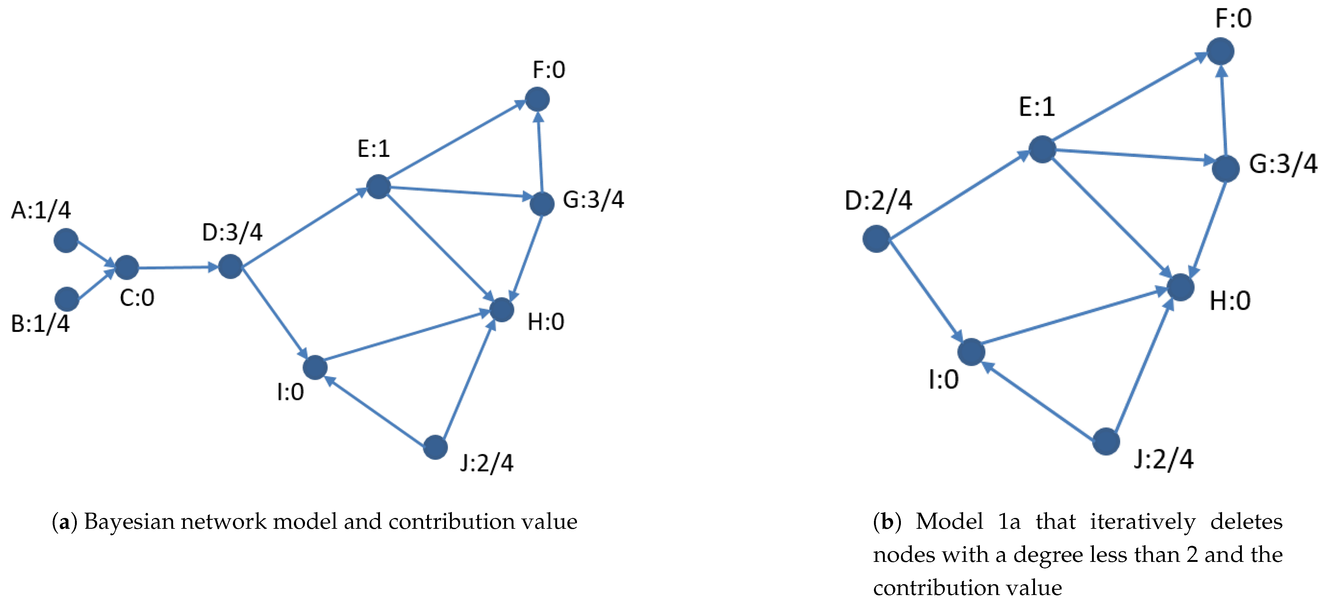
The Bayesian network model shown in Figure 1a has 10 nodes, among which the nodes with the largest degree are E and H, both are 4; the nodes with the smallest degree are A and B, both are 1. There are four sink nodes in the graph: nodes C, F, H, and I. The loop-cutting contribution of the sink nodes is 0. The loop-cutting contribution of other nodes is their node degree divided by 4, the value of largest degree in G. In Figure 1a, the loop-cutting contribution of each node is marked. A node with a degree less than 2 in the graph have no loops and cannot be an element of loop cutset. we call nodes with degree less than 2 interference nodes. Not only are these interference nodes cannot be selected into the loop cutset themselves, but they also have a negative impact on the loop-cutting contribution of other nodes. Interference nodes contribute unreasonable degrees to other nodes. The new model obtained after iteratively removing the interference nodes can get more accurate loop-cutting contribution of nodes. Figure 1b shows the new model without interference nodes and the loop-cutting contribution of each node. It can be seen from the figure that the difference in the loop-cutting contribution of node D in Figure 1a,b is still relatively large, which are 3/4 and 2/4 respectively. The reason is that the new model removes the interference nodes A, B, and C.
In the loop cutset solving process, when some elements of the loop cutset are determined, the loop-cutting contribution of other nodes will change. The nodes (sink node) with a contribution of 0 still has a contribution degree of 0; the loop-cutting contribution of other nodes changes because the number of loops in which they are located has changed. Based on the theory of [13], we simplify, subtract the shared nodes number and adjacent edges with the known loop cutset nodes from the node degree as the changed value.
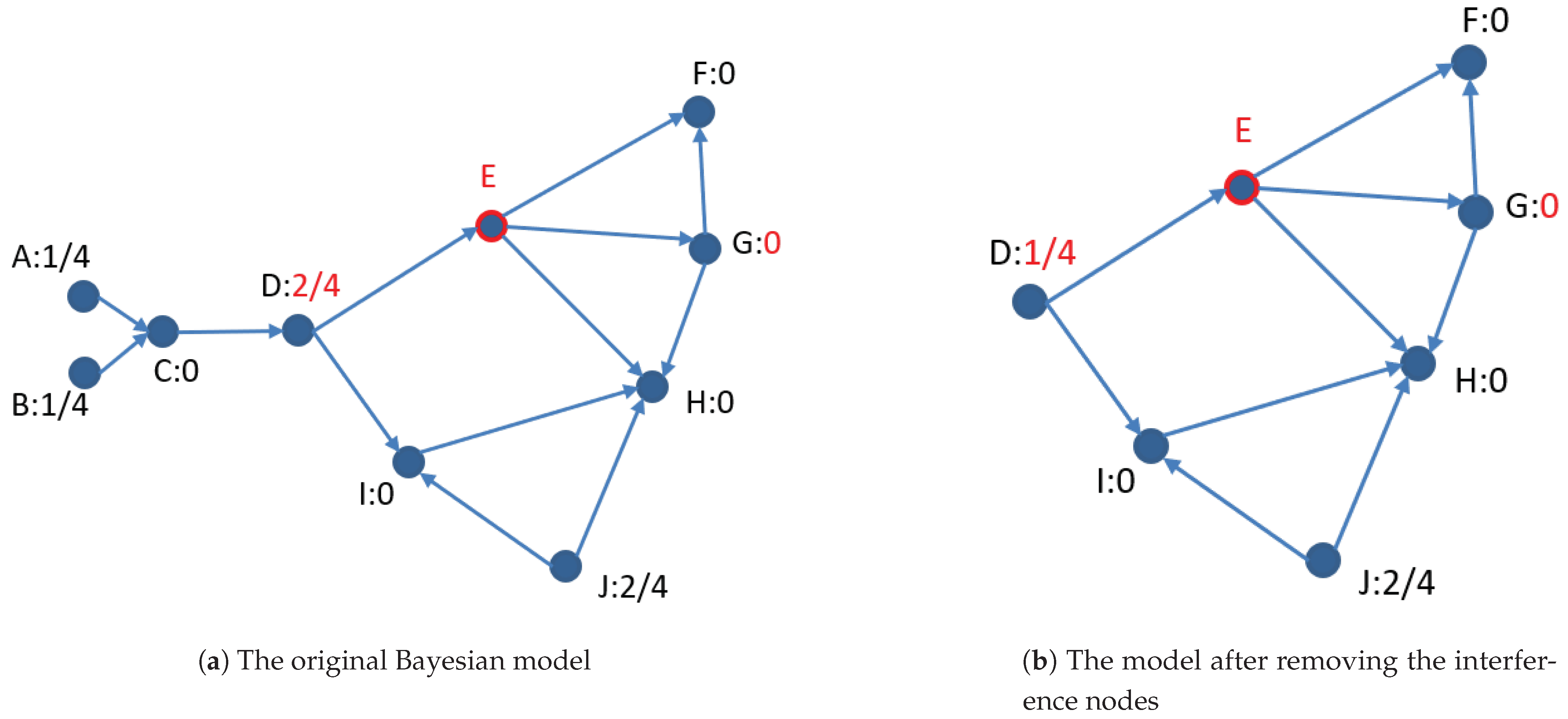
In fact, we can find from Figure 1b that the node with the greatest loop-cutting contribution is E, so in Figure 2, we take node E as the first element of the loop cutset. Figure 2a gives the loop-cutting contribution after selecting node E as a loop cutset element for the Bayesian model of Figure 1a. It can be seen that node D is the node with the largest contribution except E in Figure 2a. However, we can observe the loop where D is located has been cut by E. As mentioned above, it is because of the interference effects of nodes A, B, and C. For the model without the interference nodes given in Figure 1b, we calculate the loop-cutting contribution of each node after selecting E into the loop cutset and mark them in Figure 2b. It can be seen that the loop-cutting contribution of node D has been reduced to 1/4, and the contribution of nodes G also become 0.
Before discussing the rationality of the loop-cutting contribution, we introduce the theoretical results Lemma 1, Lemma 2, and Definition 3.2 for the references [10,13] as the theoretical basis.
Lemma 1.
For a directed acyclic graph , any node with , denote the minimum loop cutset of G as S, then the probability that node v belongs to the minimum loop cutset S satisfies the following relationship:
where and are the numbers of nodes and edges, respectively.
In a Bayesian network, a loop cutset is a collection of nodes. After the set is removed, the Bayesian network is divided into several single-connected Bayesian networks. According to Lemma 1, the node degree is positively related to the probability that the node belongs to the loop cutset. Considering the relationship between the node degree and the loops in which the node is located, we can use the node degree to reflect the number of loops in which the node is in a simplified form.
Definition 5
(Shared node). For an undirected graph , , if , , , then we call is one of the shared nodes of . Similarly, in a directed graph , , if , or , or , then we call is one of the shared nodes of [10].
Lemma 2.
For a directed acyclic graph , , denote the minimum loop cutset of G as S, then the probability that the nodes belong to the minimum loop cutset S is related to the number of the shared nodes between the two nodes. The greater the shared nodes number is, the smaller the probability.
When Bayesian networks change, the node’s loop-cutting contribution changes accordingly. According to Lemma 2, the probability that two nodes belong to the loop cutset decreases as the number of shared nodes between the two nodes increases. Then when we have a node selected as a loop cutset element, the loop-cutting contribution of another node also decreases as the number of shared nodes increases.
Based on the shared node theory, we define the loop-cutting contribution of the node-pair.
Definition 6
(Node-pair Loop-cutting Contribution). For a directed graph , , for the node-pair , if the number of the parents of u or v is greater than or equal to 2, then the node-pair’s loop-cutting contribution is 0; otherwise, the node-pair’s loop-cutting contribution is as follows:
where is the number of loops containing the node u and v at the same time. To simplify, we express the loop-cutting contribution of a node-pair as the following form, which is the sum of the contribution of the two nodes minus the shared nodes number and edge existence function .
where is the number of the shared nodes between two nodes; the value range of the edge existence function is 0–1 value. When there is an adjacent edge between two nodes, the value is 1, otherwise, it is 0, i.e.:
4. The Contribution Function Algorithm
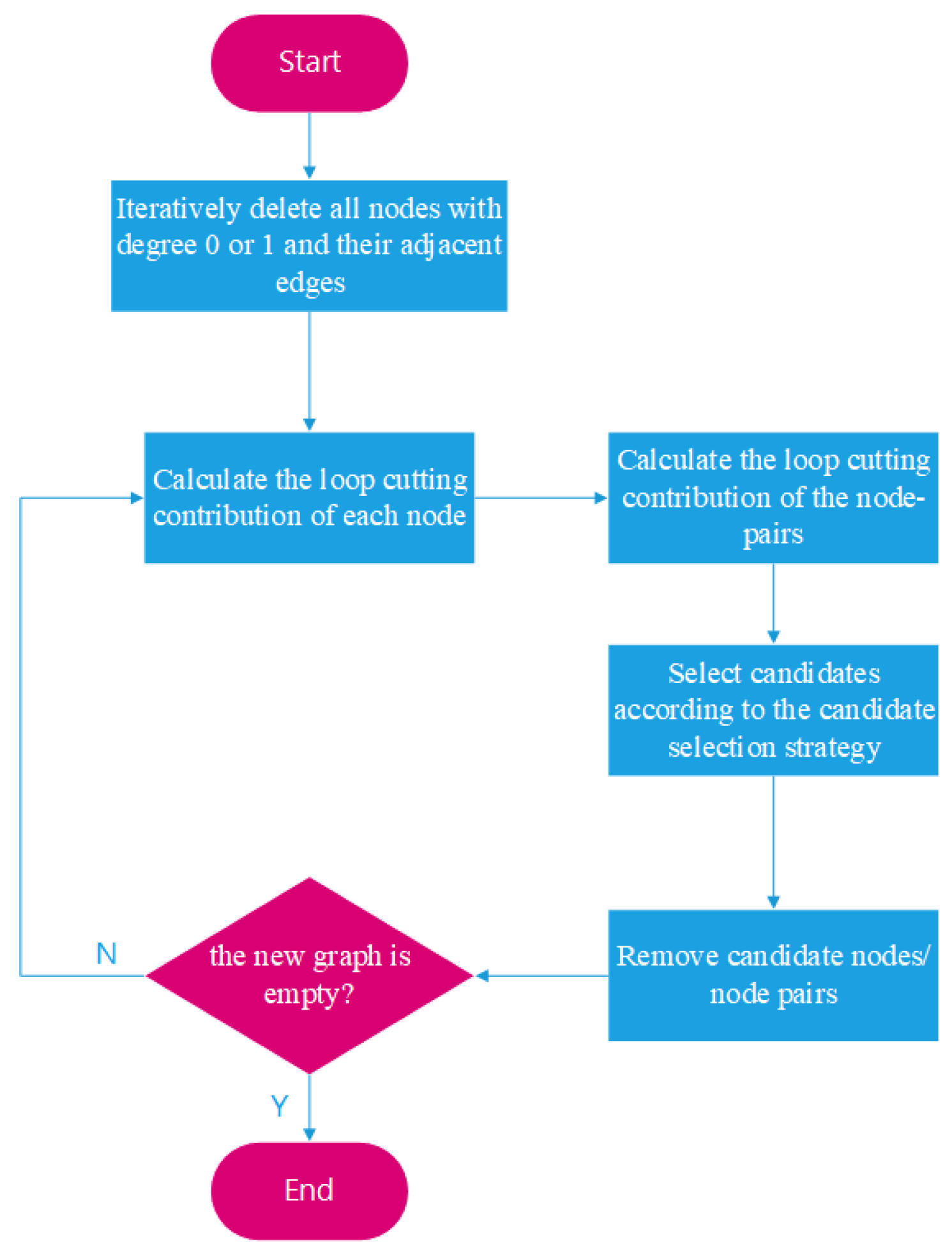
Based on the definition of the loop-cutting contribution of nodes and node-pairs proposed in Section 3, we propose an algorithm for solving the approximate minimum loop cutset: The Contribution Function Algorithm (CFA). The algorithm steps are as follows: Step 1: Iteratively delete all nodes with degree 0 or 1 and their adjacent edges from the initial graph G to obtain a new graph ; Step 2: Calculate the loop-cutting contribution of each node of the generated graph; Step 3: Find all the nodes whose loop-cutting contribution is not 0, arrange them in descending order of contribution value, and calculate the loop-cutting contribution of the node-pairs of the first N nodes. Step 4: Select candidate nodes or node-pairs according to the candidate selection strategy; Step 5: Remove candidate nodes or node-pairs and generate a new graph; Step 6: If the new graph is empty, end; if not, repeat steps 2 to 5. Figure 3 shows the algorithm flowchart.
The candidate selection strategy is the core principle of the algorithm, and its purpose is to select the most suitable nodes or node-pairs from the graph as the loop cutset candidates. When implementing this strategy, users need to specify two parameters first: and . The strategy implementation steps are as follows:
Step 1: Find all nodes whose loop-cutting contribution value is not 0, and arrange them in descending order of contribution. Examine the contribution function value of the two or two pairs of the first N nodes. among them, is a value between 0 and 1, which can be given by the user and used to take the corresponding ratio of the previous node, and N is determined by:
Step 2: If the maximum contribution value of node-pairs is greater than times the maximum contribution value of the nodes, the node-pair with the largest contribution function value is selected as the loop cutset candidates; otherwise, the node with the largest contribution function value is selected as the loop cutset candidate. The parameter is a value between 1 and 2, which can be set by the user. This value is related to the efficiency and effectiveness of the algorithm.
Step 3: When the loop-cutting contribution function values of several node-pairs are the same as the maximum value, the one with no common edge between the nodes is selected as the candidate node pair.
The pseudo-code of the Contribution Function algorithm is as follows (Algorithm 1):
| Algorithm 1 Contribution Function Algorithm |
|
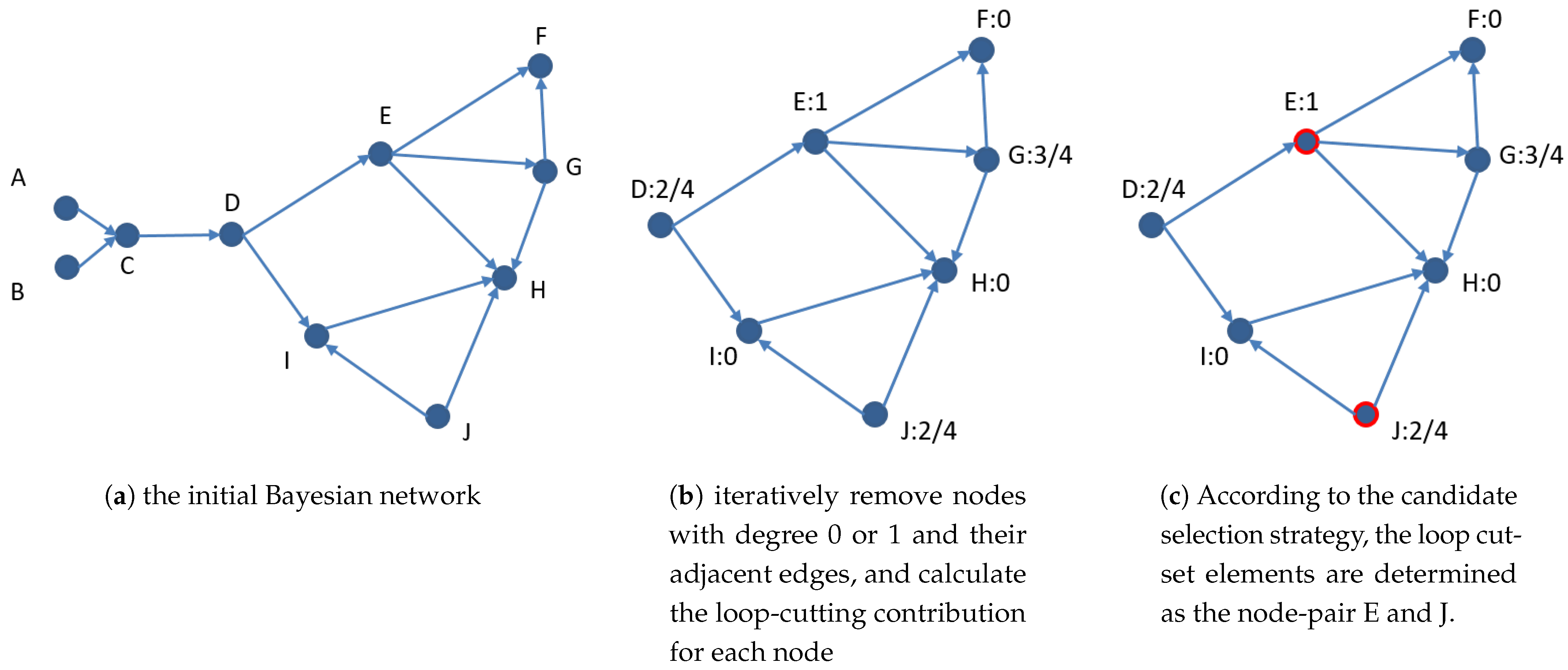
Figure 4 applies the CFA algorithm to the Bayesian network model given in Figure 1. Among them, Figure 4a gives the initial graph, Figure 4b gives the model after iteratively deleting nodes with degree 0 or 1 and their adjacent edges, and the loop-cutting contribution is calculated for each node. In Figure 4b, we know that node E has the greatest loop-cutting contribution. Next, we calculate the contribution values of the node-pairs for each node and the E pair. For the node-pair E and D, the contribution of node E is 1, and the contribution of node D is 2/4, and they have no shared node and one adjacent edge, then the contribution of node-pair ED is . Similarly, for the node-pair E and F, the contribution is 0; for the node-pair E and G, the contribution is ; for the node-pair E and H, the contribution is 0; for the node-pair E and I, the contribution is 0; for the node-pair E and J, the contribution is . Among them, the node-pairs ED and EJ have the same contribution and are the largest. However, because ED has adjacent edge while EJ has no adjacent edge. According to the candidate selection strategy step 3, the loop cutset elements are determined as the node-pair E and J, as shown in Figure 4c.
The parameters and in the algorithm control the range of node-pairs compared in the algorithm. However, in the example in Figure 4, for a comprehensive example, the node is compared to all considerations, so it does not involve the selection of parameters.
In the worst case, the time complexity of using the CFA algorithm to find the smallest loop cutset is . But under normal circumstances, thanks to the strategy of selecting node-pairs as candidates, the time complexity of CFA is much less than the worst-case time complexity. In the experimental analysis in Section 5, we will conduct an experimental analysis of the time complexity of the CFA algorithm.
5. Experiments
In the experiments, we randomly generate the Bayesian networks by using the algorithm in reference [3]. The generation parameters are the number of nodes, the number of edges, and the value range of the nodes.
Here we introduce the MGA algorithm to compare and analyze the solution results of the CFA algorithm. The MGA algorithm is a greedy algorithm proposed by Becker and Geiger in 1996 to solve the loop cutset problem [5]. For solving the loop cutset problem, researchers have made many efforts on three classes of solving algorithms: heuristic algorithms, random algorithms and precise algorithms. According to the data provided in the experimental part of the reference [13], the MGA algorithm is the most outstanding in terms of accuracy and solution efficiency of the results, so we choose the MGA algorithm as a reference group in the experiments.
The first half of the experiments, with MGA as the reference group, analyzes the result accuracy and calculation efficiency of the CFA algorithm, while the second part of the experiments studies the parameters and and analyzes the effect of the parameters on the experimental results by using the method of two-factor variance analysis.
We introduce a parameter that characterizes the complexity of the graph [13]. Assuming that a simple graph , the number of nodes is p, and the number of edges is q, then p and q satisfy the relationship . Define a new parameter , satisfying . The range of is , when its value is 0, G is a trivial graph; when its value is 1, G is a complete graph. It can be seen from this definition that the parameter can describe the degree of saturation of the edges in the graph, and measure the complexity of the graph from the perspective of the edge saturation.
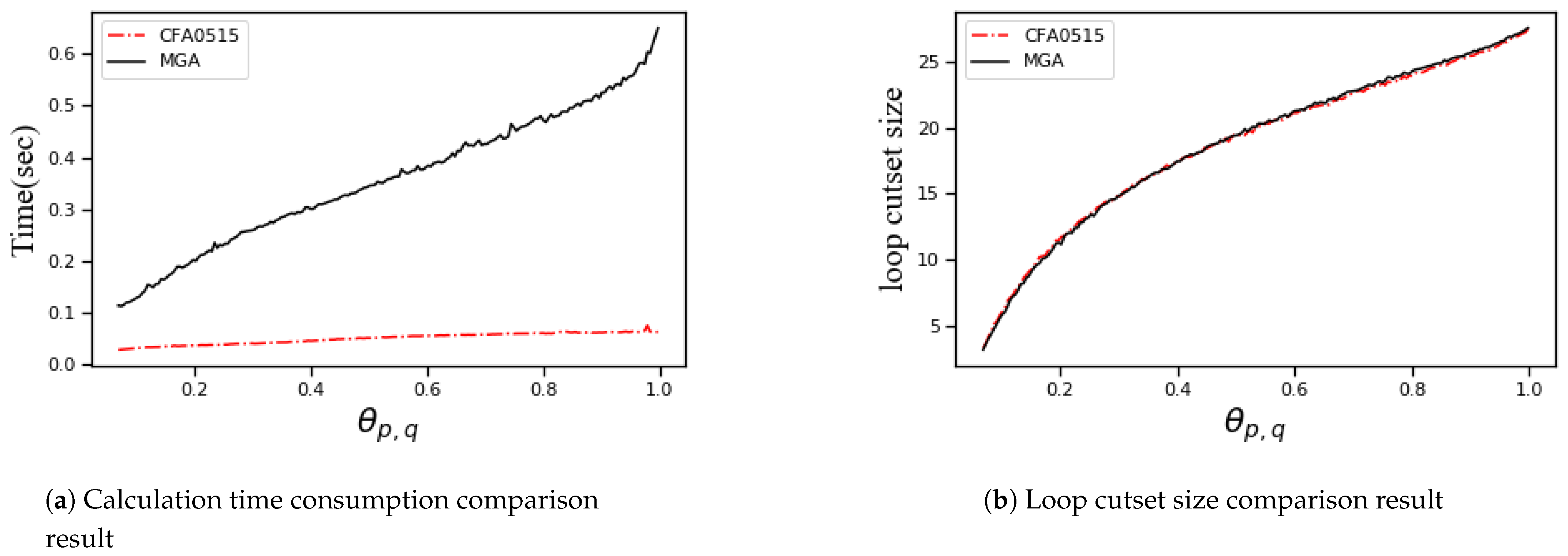
In the experiments, first, we analyze the effect of the CFA algorithm. In the CFA algorithm, we take as 0.5 and as 1.5. We randomly generate Bayesian networks with 30 nodes and an increasing number of edges and apply the CFA and the MGA to the Bayesian networks, respectively. The comparison of the results is shown in Figure 5. The red dotted line on the label in Figure 5 indicates “CFA0515”, where CFA represents the CFA algorithm, ref. [5] represents the parameter value is 0.5, 15 represents the parameter value is 1.5. The same usage is used in the following figures. In this group of Bayesian networks, we fix the number of nodes to 30 and increase the number of edges from 30 to 435. Then the edge saturation of the model gradually increases, and the value of the parameter also increases (When the number of edges is 435, the value of is 1). For each different number of edges, we randomly generate 100 Bayesian networks, apply the CFA and the MGA to these Bayesian networks, respectively. We average the experimental data of these 100 solutions as the loop cutset size or calculation time corresponding to the corresponding parameter . The result of the algorithm takes into account the size of the loop cutset and the time consumption of the calculation, and the independent variable is the parameter .
It can be seen from Figure 5 that the CFA is far superior to MGA in time cost, and the accuracy of the results is comparable to that of MGA. The calculation time of the CFA has always been less than that of the MGA, and the gap becomes larger as the graph becomes more complex. Through this experiment, we can conclude that the CFA is more efficient than the MGA. The main reason is that the CFA algorithm selects taking node-pairs as candidates.
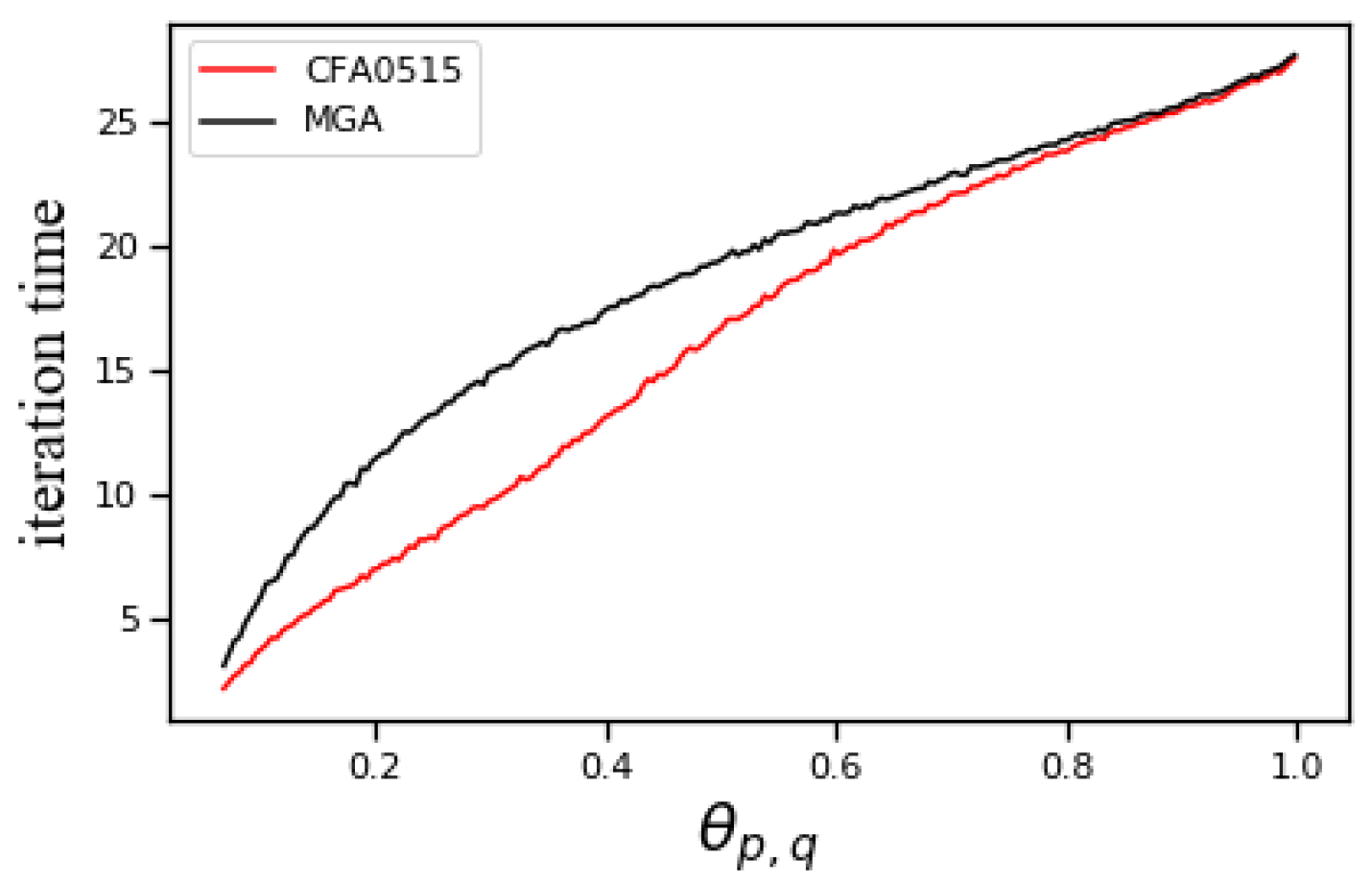
To more accurately examine the time cost of CFA and MGA, we conduct statistical analysis on the iteration number of the two algorithms. Figure 6 shows the comparison results of the iteration number of CFA (the parameters take values 0.5 and 1.5 respectively) and MGA. It can be seen that the iteration number of CFA is less than that of MGA, and the gap between the two changes with the complexity of graphics. When the graph is close to the edge saturation, the iteration times of the two are close.
The time efficiency of the CFA algorithm is improved. On the one hand, the introduction of shared nodes reduces the number of iterations. On the other hand, it is the overall convenience of judging the selection of candidate elements. The combined effect of the two aspects makes the CFA algorithm effective and efficient.
In the above experiments, we examined the comparison results of the CFA and the MGA when and were 0.5 and 1.5, respectively. In the following experiments, we focus on the different effects of the parameters and on the experimental results in the CFA. Below we keep the value of unchanged and change the value of , then keep the value of unchanged and change the value of , and examine the results, respectively. In the following three sets of experiments, the algorithm is still aimed at the randomly generated Bayesian networks with 30 nodes and gradually increasing edges, and the reference independent variable for the comparison of results is still the parameter .
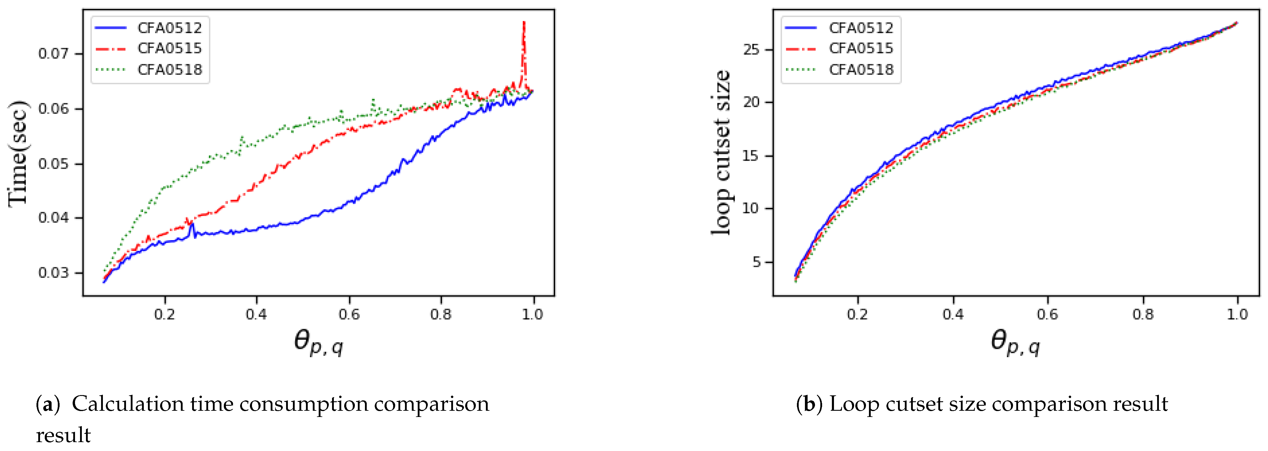
Figure 7 shows the comparison of the results of implementing the CFA on the generated Bayesian networks while keeping unchanged and changing the value of . It can be seen from Figure 7 that keeping unchanged, as the parameter increases, the size of the loop cutset decreases, and the time consumption increases.
Figure 8 shows the comparison of the results of implementing the CFA on the generated Bayesian networks while keeping unchanged and changing the value of . It can be seen from Figure 8 that keeping unchanged, as the parameter increases, the size of the loop cutset decreases, and the time consumption increases.
To further study the influence of and on the algorithm results, we use a two-way analysis of variance to analyze the experimental data. In the analysis, we fixed the nodes number of the Bayesian networks to 30, to 0.2023, and the edge number is 88. The values of the two parameters are 0.2, 0.8, 0.5 for , and 1.2, 1.5, 1.8 for . There are 9 combinations of the two-parameter, and the test is repeated 100 times for each combination. The two-factor analysis of variance is performed on the loop cutset size and calculation time obtained from the experiment. Table 1 below is the variance analysis of the two parameters on the loop cutset size, and Table 2 is the variance analysis of the two parameters on the calculation time.
According to the variance analysis table, for the loop cutset size, because the probability values of and are less than 0.05, the different values of and have significant differences in the size results; the probability of the interaction between the two is greater than 0.05, and there is no significant interaction effect between the two; for the calculating time, the probability values of and are less than 0.05, so the different values of and have significant differences in the time results; the probability of the interaction between the two is less than 0.05, so the two have significant interaction effects on them. This conclusion corresponds to the algorithm design. The parameter determines the range of node-pairs. The larger the parameter, the more node-pairs are considered, and vice versa. The determines the conditions for the selection of node-pairs. The larger the , the more difficult it is for a node-pair to be selected, and vice versa the easier it is.
In summary, the CFA algorithm has a smaller time cost than MGA, and its accuracy is comparable to MGA. It is an effective algorithm for solving cut sets. The two parameters of the CFA algorithm have an impact on the algorithm results. Users can adjust the algorithm effect by setting the parameters.
6. Conclusions
This paper proposes the loop-cutting contribution of nodes and functions. With this tool, we have an overall grasp of the contribution of all nodes in the network; based on the theory of shared nodes, we propose the loop-cutting contribution of node-pairs, consider the impact on loop-cutting from the perspective of node-pairs. Based on the above theory, this paper proposes a loop cutset solving the algorithm based on the loop-cutting contribution, which can evaluate the contribution of all nodes, and select loop cutset candidates with node-pair as the unit. This helps improve algorithm efficiency.
The experimental part analyzes the parameters of the CFA algorithm and proves that the algorithm results can be adjusted by setting the parameters. The data experiments can prove that the algorithm results are effective, and the efficiency is improved, especially the time efficiency is better than similar existing algorithms (such as MGA). The CFA can be used in the subsequent work of solving loop cutsets, which is helpful to the structural analysis of the Bayesian network and is helpful to the further improvement of the Bayesian inference.
Although the theory of loop-cutting contribution proposed in this paper is supported by related theories, the theoretical proof needs to be further improved. The next step is recommended: 1. Further analysis of the key parameters in the CFA to find more suitable values; 2. Try to find loop cutsets that can achieve a certain effect, so that the next step of reasoning will be smoother.
Author Contributions
Conceptualization, J.W. and Y.N.; methodology, J.W. and Y.N.; software, J.W.; validation, J.W.; formal analysis, J.W. and W.X.; investigation, J.W. and Y.N.; data curation, J.W. and W.X.; writing—original draft preparation, J.W.; writing—review and editing, Y.N. and W.X.; visualization, J.W. and W.X.; supervision, Y.N. and W.X.; project administration, Y.N.; funding acquisition, Y.N. All authors have read and agreed to the published version of the manuscript.
Funding
This work was supported by the National Natural Science Foundation of China, 11971386.
Institutional Review Board Statement
Not applicable.
Informed Consent Statement
Not applicable.
Conflicts of Interest
The funders had no role in the design of the study; in the collection, analyses, or interpretation of data; in the writing of the manuscript, or in the decision to publish the results.
Abbreviations
The following abbreviations are used in this manuscript:
| MDPI | Multidisciplinary Digital Publishing Institute |
| DOAJ | Directory of open access journals |
| TLA | Three letter acronym |
| LD | linear dichroism |
References
- Cooper, G.F. The computational complexity of probabilistic inference using Bayesian belief networks. Artif. Intell. 1990, 42, 393–405. [Google Scholar] [CrossRef]
- Razgon, I. Exact computation of maximum induced forest. In Scand. Workshop Algorithm Theory; Springer: Berlin/Heidelberg, Germany, 2006. [Google Scholar]
- Suermondt, H.J.; Gregory, F.C. Probabilistic inference in multiply connected belief networks using loop cutsets. Int. J. Approx. Reason. 1990, 4, 283–306. [Google Scholar] [CrossRef] [Green Version]
- Suermondt, J.; Gregory, F.C. Updating probabilities in multiply-connected belief networks. arXiv 2013, arXiv:1304.2377. [Google Scholar]
- Becker, A.; Dan, G. Optimization of Pearl’s method of conditioning and greedy-like approximation algorithms for the vertex feedback set problem. Artif. Intell. 1996, 83, 167–188. [Google Scholar] [CrossRef] [Green Version]
- Becker, A.; Reuven, B.-Y.; Dan, G. Randomized algorithms for the loop cutset problem. J. Artif. Intell. Res. 2000, 12, 219–234. [Google Scholar] [CrossRef]
- Freeman, L.C. Centrality in social networks conceptual clarification. Soc. Netw. 1978, 1, 215–239. [Google Scholar] [CrossRef] [Green Version]
- Barrat, A.; Barthélémy, M.; Pastor-Satorras, R.; Vespignani, A. The architecture of complex weighted networks. Proc. Natl. Acad. Sci. USA 2004, 101, 3747–3752. [Google Scholar] [CrossRef] [PubMed] [Green Version]
- Newman, M.E.J. Scientific collaboration networks. II. Shortest paths, weighted networks, and centrality. Phys. Rev. E 2001, 64, 016132. [Google Scholar] [CrossRef] [PubMed] [Green Version]
- Wei, J.; Nie, Y.; Xie, W. Shared Node and Its Improvement to the Theory Analysis and Solving Algorithm for the Loop Cutset. Mathematics 2020, 8, 1625. [Google Scholar] [CrossRef]
- Bidyuk, B.; Dechter, R. Cutset sampling for Bayesian networks. J. Artif. Intell. Res. 2007, 28, 1–48. [Google Scholar] [CrossRef] [Green Version]
- Pearl, J. Models, Reasoning and Inference; Cambridge University Press: Cambridge, UK, 2000. [Google Scholar]
- Wei, J.; Nie, Y.; Xie, W. The Study of the Theoretical Size and Node Probability of the Loop Cutset in Bayesian Networks. Mathematics 2020, 8, 1079. [Google Scholar] [CrossRef]
Figure 1.
Bayesian network models and node’s loop-cutting contribution values.

Figure 2.
The loop-cutting contribution of each node after selecting node E as one loop cutset element.
Figure 2.
The loop-cutting contribution of each node after selecting node E as one loop cutset element.

Figure 3.
The algorithm flowchart of CFA.

Figure 4.
Apply the CFA algorithm to the Bayesian network given in Figure 1.
Figure 4.
Apply the CFA algorithm to the Bayesian network given in Figure 1.

Figure 5.
Randomly generate Bayesian networks with 30 nodes and gradually increasing the number of edges, apply the CFA and the MGA to the Bayesian networks, respectively.
Figure 5.
Randomly generate Bayesian networks with 30 nodes and gradually increasing the number of edges, apply the CFA and the MGA to the Bayesian networks, respectively.

Figure 6.
The comparison results of the iteration number of CFA (the parameters are respectively 0.5 and 1.5) and MGA.
Figure 6.
The comparison results of the iteration number of CFA (the parameters are respectively 0.5 and 1.5) and MGA.

Figure 7.
Keep the unchanged and change the value of , the comparison chart of the results of the CFA algorithm.
Figure 7.
Keep the unchanged and change the value of , the comparison chart of the results of the CFA algorithm.

Figure 8.
Keep the unchanged and change the value of , the comparison chart of the results of the CFA algorithm.
Figure 8.
Keep the unchanged and change the value of , the comparison chart of the results of the CFA algorithm.


Table 1.
The variance analysis of the two parameters on the loop cutset size.
| Source of Variation | Sums of Squares | df | Mean Square | F | p-Value |
|---|---|---|---|---|---|
| 50.60222 | 2 | 25.30111 | 19.69569 | 4.26539 | |
| 62.08222 | 2 | 31.04111 | 24.164 | 6.03149 | |
| Interaction | 9.917778 | 4 | 2.479444 | 1.930127 | 0.103376098 |
| Error | 1144.58 | 891 | 1.284602 | ||
| Total | 1267.182 | 899 | 1.409546 |
Table 2.
The variance analysis of the two parameters on the calculation time.
| Source of Variation | Sums of Squares | df | Mean Square | F | p-Value |
|---|---|---|---|---|---|
| 0.003437 | 2 | 0.001719 | 152.5218 | 1.08196 | |
| 0.013694 | 2 | 0.006847 | 607.6856 | 3.4333 | |
| Interaction | 0.000492 | 4 | 0.000123 | 10.91249 | 1.21607 |
| Error | 0.010039 | 891 | 1.13 | ||
| Total | 0.027662 | 899 | 3.08 |
Publisher’s Note: MDPI stays neutral with regard to jurisdictional claims in published maps and institutional affiliations. |
© 2021 by the authors. Licensee MDPI, Basel, Switzerland. This article is an open access article distributed under the terms and conditions of the Creative Commons Attribution (CC BY) license (http://creativecommons.org/licenses/by/4.0/).
Share and Cite
MDPI and ACS Style
Wei, J.; Xie, W.; Nie, Y. An Algorithm Based on Loop-Cutting Contribution Function for Loop Cutset Problem in Bayesian Network. Mathematics 2021, 9, 462. https://doi.org/10.3390/math9050462
AMA Style
Wei J, Xie W, Nie Y. An Algorithm Based on Loop-Cutting Contribution Function for Loop Cutset Problem in Bayesian Network. Mathematics. 2021; 9(5):462. https://doi.org/10.3390/math9050462
Chicago/Turabian StyleWei, Jie, Wenxian Xie, and Yufeng Nie. 2021. "An Algorithm Based on Loop-Cutting Contribution Function for Loop Cutset Problem in Bayesian Network" Mathematics 9, no. 5: 462. https://doi.org/10.3390/math9050462
Note that from the first issue of 2016, this journal uses article numbers instead of page numbers. See further details here.