Determining Safe Withdrawal Rates for Post-Retirement via a Ruin-Theory Approach

Abstract

To ensure a comfortable post-retirement life and the ability to cover living expenses, it is of utmost importance for individuals to have a clear understanding of how long their pre-retirement savings will last. In this research, we employ a ruin-theory approach to model the inflows and the outflows of retirees’ portfolios. We track all transactions within the portfolios of retired clients sourced by a registered investment provider to Canada’s Financial Wellness Lab at Western University. By utilizing an advanced ruin model, we calculate the mean and the median time it takes for savings to be exhausted, the probabilities of exhaustion of funds within the retirees’ expected remaining lifetime while accounting for the observed withdrawal rates, and the deficit at ruin if a retiree has used up all of their savings. We also account for gender as well as for the risk tolerance of retired clients using a K-Means clustering algorithm. This allows us to compare the financial outcomes for female and male retirees and to enhance some findings in the literature. In the final phase of our study, we compare the results obtained by our methodology to the 4% rule which is a widely used approach for post-retirement spending. Our results show that most retirees can withdraw safely more than they currently do (around 2.5%). A withdrawal rate of about 4.5% is proved to be safe, but it might not provide sufficient income for most retirees since it yields approximately CAD 20,000 per year for male retirees in the highest risk tolerance group who withdraw about 4.5% annually.

1. Introduction

The motivation behind this research stems from the importance of being able to afford the expenses of life after retirement as well as the quality of life in this period. Our findings are based on data for over 4500 retirees from a registered investment provider. The data include the personal information of the retired clients, the initial composition of their portfolios, and subsequent transactions for a period of about three years. Our goal is to gain insights into how successful different investment and spending strategies are. These insights are to be utilized subsequently for advising retired clients whether they need to improve the way that they are spending: Are they withdrawing in a safe way or do they need to be more conservative? Are their investment strategy appropriate for their stage in life? We note that although this study is only based on the retired clients of this particular registered investment provider, by comparing some of their characteristics to characteristics of the overall Canadian population, we can conclude that our data sample is representative in many respects for Canadians in general.

In this paper, we employ an advanced ruin-theory approach for modeling retirees’ deposits and withdrawals to obtain the mean and median time until their savings are exhausted, i.e., until financial ruin. Moreover, our results include annual retirement incomes, mean and median time to exhaustion of savings, ruin probabilities, deficit at ruin if it occurs, and annual withdrawal rates, while we consider gender differences and the average lifespan of Canadians as well as the risk tolerance of the retirees in all our analyses.

The model that we use is inspired by the risk-theory model proposed by Labbé and Sendova (2009). Studies on this model provide several risk quantities from which one can evaluate how risky the business of an insurance company is. These quantities also suggest ways for mitigating the associated risks. Based on our data analysis, we need to incorporate dependence between certain random variables; therefore, the risk-theory model from Labbé and Sendova (2009) needs to be modified accordingly. In addition, as we utilize real data, our simulations are based on non-parametric distributions in the way they arise from the data. The methodologies that we develop here are applicable to other data sets, which might come from private institutions or from governmental agencies, concerning the Canadian population or the populations of other countries. One needs to perform the analyses described in this article to reach relevant conclusions. Also, given the body of literature in actuarial risk theory, there are other risk quantities, not included in this paper, that have been studied and could contribute to more informed decisions for retirees.

After a literature review in next section, we conduct some preliminary analysis of the data in Section 3. Following that, we categorize the retirees into groups based on two crucial factors: their gender and their risk tolerance using the K-Means clustering algorithm. In Section 4, we describe the ruin model that we propose in this paper. The simulation algorithm, utilized distributions, and results are provided in Section 5. Ultimately, in Section 6, we provide discussions and conclusions.

2. Literature Review

As individuals approach retirement, a crucial concern arises regarding the sustainability of their financial resources over the long term. The determination of a safe withdrawal rate is a pivotal aspect of financial planning, aimed at ensuring a comfortable and secure post-retirement. Over the years, extensive research has been conducted in the fields of Finance, Economics, Financial Mathematics, and Actuarial Science to develop models that can accurately determine or maximize the safe withdrawal rate while minimizing the probability of a premature exhaustion of funds.

One important paper in this area is Bengen (1994). This article marks a significant milestone and introduces the concept of the “$4\%$ rule”. This research demonstrates that a withdrawal rate of $4\%$ of the initial portfolio value, adjusted annually for inflation, has a high likelihood of sustaining a retirement portfolio for a 30-year period. Subsequent studies have built upon this foundation, exploring alternative withdrawal strategies, incorporating diverse assets, and accounting for varying economic conditions to enhance the methodology for determining a safe withdrawal rate.

Milevsky et al. (2006) combine utility maximization from insurance economics with shortfall-minimizing investment and hedging strategies from finance and risk management. The objective is to find the optimal investment and annuitization approach for fixed consumption, with a focus on asset allocation and annuitization strategies to minimize the probability of bankruptcy. The research is closely related to portfolio management. Another study is Moore and Young (2006) where asset allocation is emphasized once again along with a proposed method to minimize the probability of bankruptcy. It is observed that longer-term investors should have higher allocations to riskier assets. However, the study’s assumptions of deterministic mortality and constant, risk-free volatility, and rate of return are not realistic for the long-term horizon.

Subsequently, Pfau (2011) examines 109 years of financial market data from 17 developed countries to gain a broader perspective. In that study, 4% withdrawal rate is found to be risky internationally, providing safety in only 4 out of 17 countries. Additionally, a fixed asset allocation split between stocks and bonds fails in all countries. This research emphasizes the significance of considering international factors when determining safe retirement withdrawal rates. Further, Finke et al. (2011) explores the relationship between risk tolerance and retirement income decisions. They find that the 4% withdrawal rate is suitable for risk-averse clients with moderate guaranteed income. Risk-tolerant investors prefer higher withdrawal rates and a riskier portfolio in retirement.

Van Appel et al. (2021) rely on historical data and Monte Carlo simulation, with asset allocation playing a crucial role. The probability of portfolio success is assessed based on different asset mixes (equity, bonds, cash), highlighting the potential benefits of equity in achieving success for higher withdrawal rates. Longevity and management fees are also taken into consideration. A different approach in the study Van Appel and Maré (2022) aims to determine a withdrawal rate that prevents funds from running out and maintains a comfortable lifestyle. Instead of relying on historical data, forward-looking risk-neutral and real-world distributions derived from option prices on South African top 40 indexes are used. By employing this approach, a safe withdrawal rate of up to 7% is deemed feasible, significantly higher than the commonly used 4% obtained from simulation and historical data. Another study by Anarkulova et al. (2022) examines retirement spending rules using a data set from 38 developed countries. They find that a 65-year-old couple willing to accept a 5% chance of bankruptcy can only withdraw 2.26% annually, much lower than the commonly advised 4% rule.

Also in 2022, Schabort (2022) examines the sequence of return risk (SOR risk) in South African retirement portfolios using five asset allocation strategies. Simulations from 1991 to 2020, with 10,000 trials, assessed sustainable withdrawal rates and actuarial coverage ratio. Geographic diversification reduced SOR risk, and the dynamic cash buffer strategy outperformed others in mitigating this risk compared to benchmarks. Another study, Stocker (2023), combines income from a Defined Benefit (DB) pension with an investment portfolio to maintain constant inflation-adjusted total required income (IR). Adding income from a DB pension without inflation protection extended the retirement income period significantly, with the maximum safe withdrawal rate increasing by about 0.6 to 0.8 percentage points per percentage point of DB pension income, based on the level of inflation protection.

There is also some research in the area of safe withdrawal rate based on the data from India. For example, Saraogi (2022) determines a safe withdrawal rate (SWR) for Indian retirement portfolios, finding it lower than the commonly used 4% SWR for the U.S. market. For the average Indian investor, a 3% SWR is recommended, and for risk-averse investors, it should not exceed 2.6%. In Raju and Saraogi (2024), the authors redefine safe withdrawal rates for retirement planning in India, recommending a range of 3.0% to 3.5% instead of the commonly cited 4% rule. Higher equity allocations can boost SWR but also raise the risk of portfolio failure, especially beyond 3.75% withdrawal rates. Taxes on fixed deposit interest affect all-deposit portfolios. Gold is highlighted as a diversifying asset to reduce market-related risks in portfolios.

The modeling approach that we utilize in this paper is mainly based on the ruin model in Labbé and Sendova (2009). There, the authors focus on ruin theory using the expected discounted penalty function in a risk model with compound Poisson processes for modeling premiums and claims. That research establishes equations for the penalty function and explores their implications on quantities like the discounted deficit and the probability of ultimate ruin. It also investigates the case of Erlang premiums and arbitrarily distributed claims. After that, Zhang and Yang (2010) expand on the research conducted by Labbé and Sendova (2009) regarding a compound Poisson risk model with stochastic premium income. Their focus lies in the specific dependence structure between claim sizes, inter-claim times, and premium sizes within this model.

Xie and Zou (2013) introduce a risk model with dependent claim occurrences, premium sizes, and claim sizes. Assuming exponential premium sizes, they derive Laplace transforms and defective renewal equations for expected discounted penalty functions. Solutions are represented using a compound geometric distribution. They also explore subexponential claims and obtain asymptotic ruin probability formulas. Vidmar (2018), studies the ruin probability in a modified Cramer–Lundberg model, which describes the surplus process of an insurance company. The model assumes independent mixed Poisson processes for premium and claim arrival times, taking into account their respective intensities. This model introduces stochastic dependence between the total premium and claim amounts. Also, the study yields a clear expression for the ruin probability when both claim and premium sizes follow exponential distributions. Guan and Wang (2023) examine the dependence between premium numbers in consecutive periods and claim numbers in consecutive periods using integer-valued auto-regressive (IVAR(1)) and integer-valued moving average (INMA(1)) processes. Additionally, the authors establish an asymptotic formula for the finite-time ruin probability by studying the large deviations of the aggregate claims.

Finally, actuarial science and financial risk management have commonly employed copulas to represent the dependence between random variables. Notable papers discussing their applications include Bregman and Klüppelberg (2005), Denuit et al. (2006), Albrecher and Teugels (2006), Cossette et al. (2008), Albrecher et al. (2011), Chadjiconstantinidis and Vrontos (2014), and Blier-Wong et al. (2022).

3. Data and Descriptive Analysis

In this paper, we track the transactions of retirees which are provided through Canada’s Financial Wellness Lab from a registered investment provider. We use four different tables with data for different purposes. One table is utilized for retirees’ personal information such as age, gender, retirement status, etc. Two tables are related to trades and transactions and yet another table is used for the retirees’ initial wealth. The transactions are tracked over a period of three years and two months from the 15th of July of the year 2019 to the 15th of September of the year 2022.

3.1. Grouping the Retirees

Since in this context, risk tolerance is an important factor, we group the retirees based on their risk tolerance. In our data, we first assign a number to each retired client based on the risk tolerance that they have declared. The risk tolerance is stated by retirees in the form of the asset mix that they select initially. Over time, advisors or retirees themselves might adjust their asset mix with the purpose of maintaining the overall risk level of the portfolio. Assets available for purchase are classified into five groups with risk levels ranging from low to high, respectively. Thus, any retiree’s portfolio is of the format “$a\%$ in Low-risk assets, $b\%$ Low to Medium, $c\%$ Medium, $d\%$ Medium to High, $e\%$ High”. We assign numbers from 100 to 500 to the five levels from Low to High. Then by taking a summation of the product of percentage in each level and the number assigned to that level, a single number showing the risk tolerance of the retired client is obtained. The risk tolerance number could vary from 1000 to 5000, so that 1000 means the lowest and 5000 means the highest risk tolerance.

First of all, we examine whether clustering of our dataset is statistically meaningful or not. For this purpose, based on Hopkins and Skellam (1954), Gastner (2005), and Cross and Jain (1982), we use the p-value for Hopkins statistic under the null hypothesis of spatial randomness. Then, based on Kassambara (2017), we employ the K-Means clustering algorithm and after examining all features and obtaining the silhouette coefficient for all of them, we find that using only the feature of “risk tolerance” produces the best clustering for our purposes. The Elbow method and the silhouette coefficient suggest four clusters for male and four clusters for female retirees. The results of the Hopkins statistic and silhouette coefficient based on the feature “risk tolerance” and four clusters for each gender of male and female are shown in

Table 1. The results of Hopkins statistic and Silhouette Coefficient for clustering based on “risk tolerance” feature and 4 clusters.

Gender	Hopkins Statistic	Hopkins Statistic p-Value	Silhouette Coefficient
Male	0.9896	0.0	0.7392
Female	0.9928	0.0	0.7283

.

The results of Hopkins statistic p-value equal 0 for both male and female retirees, which shows that clustering based on the feature “risk tolerance” for both male and female retirees is highly relevant. Also, the silhouette coefficient, shows numbers above $0.5$ and as it is closer to 1, implying a stronger clustering algorithm performance. Considering that $0.7392$ and $0.7283$ are the resulting silhouette coefficients for male and female retirees, respectively, we may conclude that risk tolerance and gender are the most important features of our data. We have four clusters for each gender. (see Rousseeuw (1987) for more information about the silhouette coefficient). Therefore, the descriptive analysis of the data including the retirees’ personal information, trades, transactions, and initial wealth indicate that gender and risk tolerance are the factors that should determine how retirees should be grouped. As a result, we have eight groups of retirees in total (four groups of male and four groups of female). As we explained previously, we assigned a single number indicating the risk tolerance to each retiree, and then by grouping them using clustering and the feature of risk tolerance, depending on their risk tolerance, they belong to different groups. In

Table 2. Descriptive analysis for male and female retirees based on different groups of risk tolerance.

	Group	Risk Tolerance	Counts	Average of Age	Average of Initial Wealth
Male	1	(1000,1600)	105	78	CAD 288,646
	2	(1700,2600)	353	77	CAD 293,678
	3	(2650,3500)	1344	75	CAD 353,021
	4	(3600,5000)	365	74	CAD 424,103
Female	1	(1000,1600)	135	78	CAD 372,890
	2	(1660,2550)	412	76	CAD 364,195
	3	(2600,3200)	1305	74	CAD 342,971
	4	(3250,5000)	527	73	CAD 481,644

, one finds the risk tolerance ranges for each group and the number of retirees who fall into the relevant group. It is noteworthy that the ranges for each risk tolerance level are produced by the clustering algorithm and they are not the same for both genders. Additionally, as it might be expected, the average age of retirees in each group is inversely related to the risk tolerance level of the group.

3.2. Retirees’ Information and Initial Wealth

We have access to the retirees’ personal information such as their retirement status, gender, age, risk tolerance, etc. We only use the retired clients in this paper. A brief descriptive analysis of different groups is given in Table 2. There, it can be seen that the retirees in the highest risk tolerance group 4 for both male and female are the youngest as well as the wealthiest, while the lowest risk tolerance groups of male and female retirees are the oldest ones. These observations are consistent with guidance provided by financial advisors: younger retirees should have more wealth and take higher risk compared to older retirees who should have exhausted some of their wealth and reduced their risk tolerance.

3.3. Trades and Transactions

After analyzing the tables containing trades and transactions, two completely different patterns are detected: the table with trades shows less frequent but larger amounts, while the table with transactions shows more frequent but smaller amounts. These patterns are illustrated in Figure 1 and Figure 2. The former provides the average annual number of trades and transactions (deposits and withdrawals) split by gender, while the latter exhibits the average annual amounts of trades and transactions (deposits and withdrawals) again split by gender.

Since trades and transactions are performed in a specific succession over time, time might be a meaningful notion in the present context. Thus, one might want to interpret the data as a time series. We then need to verify whether accounting for the timing of deposits and withdrawals, i.e., considering the data as time series, provides us with more insights or we can consider the data just like regular datasets without missing any important information despite not accounting for the exact timing of deposits and withdrawals. Following Ali (1987), we utilize the Durbin–Watson test to determine whether there is auto-correlation in the data. Since the results from the test reject the hypothesis of the existence of auto-correlation, it means that we can confidently consider the data as regular datasets and not like time series. The results of the Durbin–Watson test for male and female retirees are provided in

Table 3. Results of Durbin–Watson test for male retirees.

	Series of Data	Test Statistic		Series of Data	Test Statistic
	(Random Variable)			(Random Variable)
Group 1	$X_{1i}$	1.5	Group 3	$X_{1i}$	1.7
	$Y_{1i}$	1.6		$Y_{1i}$	1.7
	$X_{2k}$	1.8		$X_{2k}$	1.6
	$Y_{2k}$	2		$Y_{2k}$	1.8
Group 2	$X_{1i}$	1.5	Group 4	$X_{1i}$	1.9
	$Y_{1i}$	1.5		$Y_{1i}$	1.9
	$X_{2k}$	1.6		$X_{2k}$	1.7
	$Y_{2k}$	1.9		$Y_{2k}$	2

and

Table 4. Results of Durbin–Watson test for female retirees.

	Series of Data	Test Statistic		Series of Data	Test Statistic
	(Random Variable)			(Random Variable)
Group 1	$X_{1i}$	1.5	Group 3	$X_{1i}$	1.5
	$Y_{1i}$	1.3		$Y_{1i}$	1.5
	$X_{2k}$	1.9		$X_{2k}$	1.7
	$Y_{2k}$	1.9		$Y_{2k}$	1.8
Group 2	$X_{1i}$	1.3	Group 4	$X_{1i}$	1.3
	$Y_{1i}$	1.5		$Y_{1i}$	1.3
	$X_{2k}$	1.5		$X_{2k}$	1.6
	$Y_{2k}$	1.7		$Y_{2k}$	1.7

, respectively. We note that in the tables, by series of data $X_{1i}$ and $X_{2k}$, we mean the data related to the amounts of deposits in trades and transactions, respectively, whereas by series of data $Y_{1j}$ and $Y_{2l}$, we mean the data related to the amounts of withdrawals in trades and transactions, respectively. Figure 1 and Figure 2 show that trades are less frequent but of larger amounts while transactions are more frequent but of smaller amounts.

The test statistic of the Durbin–Watson test is a number between 0 and 4, where the test statistic equal to 2 in Table 3 and Table 4 means that there is not statistically significant auto-correlation in the series of data. Since in rare cases it occurs that the test statistic is exactly equal to 2, it is common to consider an interval around 2 to say that there is no auto-correlation in the data.

When it comes to model trades and transactions, an important issue that can play a crucial role is the correlation between the number of deposits and the number of withdrawals as well as the correlation between the amounts of deposits and withdrawals. Hence, we need to quantify the relevant correlations and evaluate whether they are significant. Figure 3 and Figure 4 display the results of Pearson correlations between the number of deposits and the number of withdrawals and the Pearson correlations between the amounts of them in different groups for males and females, respectively. Also, according to the p-value of the performed test with the null hypothesis that the underlying distributions of the samples are uncorrelated, all the correlations are statistically significant.

On the one hand, Figure 3 shows that the correlations between the number of deposits and the number of withdrawals within trades are consistently higher than the corresponding correlations within transactions. On the other hand, Figure 4 demonstrates that we cannot make such a conclusion regarding the amounts of trades and transactions as for some groups the correlations for trades are higher while for other groups the correlations for transactions are higher.

In any case, our conclusion here is that both trades’ and transactions’ numbers and amounts are highly correlated and thus, this correlation should be implemented into the stochastic model that we choose to employ.

4. Methodology

In this section, we propose a stochastic model that describes the evolution of the wealth of retirees. Namely, denote by $\left\{U\right(t);t\ge 0\}$ the amount of wealth that a retiree has at time $t.$ We adapt the model in Labbé and Sendova (2009):

$$U\left(t\right)=u+\sum _{i=1}^{N\left(t\right)}{X}_i-\sum _{j=1}^{M\left(t\right)}{Y}_j,t\ge 0.$$

(1)

where the initial surplus of a particular insurance company is $u\ge 0,$ and the premiums ${\left\{X_i\right\}}_{i=1}^{\infty }$ and the claims ${\left\{Y_j\right\}}_{j=1}^{\infty }$ occur in time according to homogeneous Poisson processes $N\left(t\right)$ and $M\left(t\right)$ with intensities $\lambda >0$ and $\mu >0$, respectively. Each of the premium sizes and the claim sizes are assumed independent and identically distributed (i.i.d.).

In this model, if no premiums or no claims occurred up to time $t,$ then $N\left(t\right)=0$ or $M\left(t\right)=0$ and in this case, obviously, ${\sum }_{i=1}^{N\left(t\right)}{X}_j=0$ or ${\sum }_{j=1}^{M\left(t\right)}{Y}_j=0$. The other assumptions of this model are the independence of the random variables $N\left(t\right),M\left(t\right),X_1,X_2,\cdots$ and $Y_1,Y_2,\cdots ,$ and the finite expectations of the premiums and the claims such that $\mu \mathbb{E}\left(X_1\right)>\lambda \mathbb{E}\left(Y_1\right)$.

In this paper, we modify model (1) and interpret it differently. Namely, $U\left(t\right)$ is a retiree’s wealth at time t and due to the two different patterns that trades and transactions follow, we have separate summations for trades and transactions. Hence,

$$\begin{array}{ccc}\hfill U\left(t\right)=u& +& \sum _{i=1}^{A_1\left(t\right)}[(1-f)X_{1i}-(1+f)Y_{1i}]+\sum _{j=1}^{B_1\left(t\right)}{Z}_{1j}^{*}\hfill \\ & +& \sum _{k=1}^{A_2\left(t\right)}(X_{2k}-Y_{2k})+\sum _{l=1}^{B_2\left(t\right)}{Z}_{2l}-{(1+r)}^{t}c,t\ge 0.\hfill \end{array}$$

(2)

Here, u is used for the retiree’s initial wealth. The annual number of deposits for trades and transactions are modeled by the random variables $N_1\left(t\right)$ and $N_2\left(t\right)$, respectively, while $M_1\left(t\right)$ and $M_2\left(t\right)$ are utilized for the annual number of withdrawals for trades and transactions, respectively. The sequences of i.i.d. random variables $X_{11},X_{12},\cdots$ and $X_{21},X_{22},\cdots$ are used for the amounts of deposits according to the trades and transactions patterns, whereas the sequences of i.i.d. random variables $Y_{11},Y_{12},\cdots$ and $Y_{21},Y_{22},\cdots$ are employed for modeling the amounts of withdrawals based on trades and transactions patterns, respectively. $f\in [0,1)$ denotes the proportion of fee associated with trades and since it is an added cost, we need to deduct that from the deposits and add that to the withdrawals. $c\ge 0$ is a constant denoting the annual commission fee subject to an annual increase rate of r. Finally, we define the remaining processes $A_1\left(t\right),B_1\left(t\right),A_2\left(t\right)$, and $B_2\left(t\right)$, and random variables $Z_{1j}$ and $Z_{2l}$ as follows:

$$\begin{array}{cc}\hfill A_1\left(t\right)=& min(N_1\left(t\right),M_1\left(t\right))\hfill \\ \hfill A_2\left(t\right)=& min(N_2\left(t\right),M_2\left(t\right))\hfill \\ \hfill B_1\left(t\right)=& max(N_1\left(t\right),M_1\left(t\right))-min(N_1\left(t\right),M_1\left(t\right))\hfill \\ \hfill B_2\left(t\right)=& max(N_2\left(t\right),M_2\left(t\right))-min(N_2\left(t\right),M_2\left(t\right))\hfill \\ \hfill Z_{1j}^{*}=& \left\{\begin{array}{cc}(1-f)X_{1i},\hfill & N_1\left(t\right)>M_1\left(t\right)\hfill \\ 0,\hfill & N_1\left(t\right)=M_1\left(t\right)\hfill \\ (1+f)Y_{1i},\hfill & N_1\left(t\right)<M_1\left(t\right)\hfill \end{array}\right.\hfill \\ \hfill Z_{2l}=& \left\{\begin{array}{cc}{X}_{2k},\hfill & N_2\left(t\right)>M_2\left(t\right)\hfill \\ 0,\hfill & N_2\left(t\right)=M_2\left(t\right)\hfill \\ Y_{2k},\hfill & N_2\left(t\right)<M_2\left(t\right)\hfill \end{array}\right.\hfill \end{array}$$

Therefore, in model (2), the first two summations are associated with the trades, while the other two summations are related to the transactions.

Based on the preliminary analysis in Section 3, we know that there are significant correlations between the annual numbers of deposits and withdrawals as well as between their amounts in both trades and transactions. Due to the different context in which the ruin model (1) is used, dependence between the random variables $N\left(t\right)$ and $M\left(t\right)$ has not been taken into account. In contrast, in the present context, it is logical (and confirmed by the data) to consider such dependence. In this paper, we incorporate the observed correlations between the random variables in our model by utilizing Frank copulas, which are employed for symmetric dependence structures.

On the one hand, the use of copulas to model dependence between random variables is very popular in actuarial science and financial risk management. For example, Albrecher and Teugels (2006) employ copulas to define the joint distribution of inter-claim times and claim amounts and the authors of Blier-Wong et al. (2022) investigate collective risk models using a copula approach, specifically focusing on cases where the dependence structure is determined by a Farlie–Gumbel–Morgenstern (FGM) copula. Other relevant studies for applications include Frees and Valdez (1998), Wang (1998), Bouyé et al. (2000), Denuit et al. (2006), and McNeil et al. (2015). Also, general references on copulas are Joe (1997) and Nelsen (2007) among others. On the other hand, in Zhang and Yang (2010), Xie and Zou (2013), Vidmar (2018), and Guan and Wang (2023), some dependency structures and different approaches to consider them are investigated.

5. Simulation and Results

In this section, we first describe the simulation algorithms which are based on our model given in Equation (2), as well as all relevant inputs such as fitted distributions for random variables and the initial wealth. After that, we present the obtained results including mean and median time to exhaustion of funds, probability of (financial) ruin, annual retirement income based on mean and median time to exhaustion of funds, deficit at ruin, and finally the annual withdrawal rates for each group of male and female retirees.

5.1. Simulation

We perform the simulations based on the described data in Section 3 and the model given in Equation (2).

After careful consideration of many parametric distributions such as the Pareto, the Log-normal, the Weibull, the Gumbel, the Burr, the Log-logistic (also known as Fisk distribution in Economics), the Dagum Type I and Type II (also known as Mielke Beta-Kappa distribution) and the Inverse Weibull, spliced distributions, and mixture distributions for modeling the amounts of deposits and withdrawals and using Kolmogorov–Smirnov (K-S) test to verify the goodness of fit, we found that none of these distributions give appropriate fit for our data. Consequently, we choose to employ non-parametric distributions for the random variables $X_{1i},Y_{1i},X_{2k},$ and $Y_{2k}$, which represent the amounts of deposits and withdrawals for both trades and transactions. Also, for the annual number of deposits and the annual number of withdrawals, i.e., $N_1\left(t\right),M_1\left(t\right),N_2\left(t\right),$ and $M_2\left(t\right)$, since the variance is much greater than the mean, the Poisson distribution could not be appropriate. Trying to fit a Negative Binomial distribution because the variance is greater than the mean, does not show a suitable result based on the p-value of the K-S test, because it does not perform well for the right tail. Hence, for these random variables and each risk tolerance group of each gender, we fit non-parametric distributions using “rv_histogram” from “Scipy.stats” in Python.

Since we have to fit a total of eight distributions in each group of the eight groups of retirees that we have, in Figure 5 and Figure 6, we only show the relevant graphs for groups 3 of male and female retirees which group contains about a half of all retirees. From Figure 5 and Figure 6, it can be seen that this kind of non-parametric distribution gives us a precise fitting at zero, as well as at the right tail. We utilize the fitted non-parametric distributions for generating all random variables that we have in the simulations.

The simulation algorithms that we design to obtain the time to exhaustion of funds, the (financial) ruin probabilities, and the deficit at ruin are shown in Algorithms 1, 2 and 3, respectively.

Algorithm 1 Simulation algorithm for time to exhaustion of funds

Time-to-ruin = $\left[\right]$ $U\left(t\right)=U\left(0\right)=u($retiree’s age)▹ The initial wealth based on the age of retiree which is an input for i in $(0,10,000)$ do     $k=\left[\right]$     for i in $(0,1000)$ do         if $U\left(t\right)\ge 0$ then Generating two pairs of joint random variables shown with $(\widetilde{N_1\left(t\right)},\widetilde{M_1\left(t\right)})$ and $(\widetilde{N_2\left(t\right)},\widetilde{M_2\left(t\right)})$ using the non-parametric distributions of input data for the frequencies and Frank Copula with input Thetas, Generating joint random variables in two 2-dimensional vectors showing with $(\widetilde{X_{1i}},\widetilde{Y_{1i}})$ and $(\widetilde{X_{2k}},\widetilde{Y_{2k}})$ using the non-parametric distributions of input data for the amounts, Frank Copula with input Thetas, with the size of $min(\widetilde{N_1\left(t\right)},\widetilde{M_1\left(t\right)})$ and $min(\widetilde{N_2\left(t\right)},\widetilde{M_2\left(t\right)})$, respectively. Generating independent random variables in two 1-dimensional vectors showing with $\widetilde{X_{1i}}$ and $\widetilde{Y_{1i}}$ using the non-parametric distributions coming from input data with the size of $\widetilde{N_1\left(t\right)}-min(\widetilde{N_1\left(t\right)},\widetilde{M_1\left(t\right)})$ and $\widetilde{M_1\left(t\right)}-min(\widetilde{N_1\left(t\right)},\widetilde{M_1\left(t\right)})$, respectively. Generating independent random variables in two 1-dimensional vectors showing with $\widetilde{X_{2k}}$ and $\widetilde{Y_{2k}}$ using the non-parametric distributions coming from input data with the size of $\widetilde{N_2\left(t\right)}-min(\widetilde{N_2\left(t\right)},\widetilde{M_2\left(t\right)})$ and $\widetilde{M_2\left(t\right)}-min(\widetilde{N_2\left(t\right)},\widetilde{M_2\left(t\right)})$, respectively. Calculating $U\left(t\right)=U\left(t\right)+{\sum }_{i=1}^{A_1\left(t\right)}[(1-f)\times X_{1i}-(1+f)\times Y_{1i}]+{\sum }_{j=1}^{B_1\left(t\right)}{Z}_{1j}^{*}+{\sum }_{k=1}^{A_2\left(t\right)}(X_{2k}-Y_{2k})+{\sum }_{l=1}^{B_2\left(t\right)}{Z}_{2l}-{(1+r)}^{t}c$ using the numbers $f=0.007$, $c=4000$ and the rate $r=0.06$ Adding the value of $U\left(t\right)$ to the vector of k         else if $U\left(t\right)<0$ then            Break the loop         end if     end for     Adding the “length of k vector minus $0.5$” to the vector of Time-to-ruin end for Return The mean (or the median in the other case) of the vector Time-to-ruin

Algorithm 2 Simulation algorithm for ruin probabilities

Ruin-probs = 0 $U\left(t\right)=U\left(0\right)=u($retiree’s age)▹ The initial wealth based on the age of retiree which is an input for i in $(0,10,000)$ do     $k=0$     for i in $(0,$ life expectancy for retiree’s age) do         if $U\left(t\right)\ge 0$ then Generating two pairs of joint random variables shown with $(\widetilde{N_1\left(t\right)},\widetilde{M_1\left(t\right)})$ and $(\widetilde{N_2\left(t\right)},\widetilde{M_2\left(t\right)})$ using the non-parametric distributions of input data for the frequencies and Frank Copula with input Thetas, Generating joint random variables in two 2-dimensional vectors showing with $(\widetilde{X_{1i}},\widetilde{Y_{1i}})$ and $(\widetilde{X_{2k}},\widetilde{Y_{2k}})$ using the non-parametric distributions of input data for the amounts, Frank Copula with input Thetas, with the size of $min(\widetilde{N_1\left(t\right)},\widetilde{M_1\left(t\right)})$ and $min(\widetilde{N_2\left(t\right)},\widetilde{M_2\left(t\right)})$, respectively. Generating independent random variables in two 1-dimensional vectors showing with $\widetilde{X_{1i}}$ and $\widetilde{Y_{1i}}$ using the non-parametric distributions coming from input data with the size of $\widetilde{N_1\left(t\right)}-min(\widetilde{N_1\left(t\right)},\widetilde{M_1\left(t\right)})$ and $\widetilde{M_1\left(t\right)}-min(\widetilde{N_1\left(t\right)},\widetilde{M_1\left(t\right)})$, respectively. Generating independent random variables in two 1-dimensional vectors showing with $\widetilde{X_{2k}}$ and $\widetilde{Y_{2k}}$ using the non-parametric distributions with the size of $\widetilde{N_2\left(t\right)}-min(\widetilde{N_2\left(t\right)},\widetilde{M_2\left(t\right)})$ and $\widetilde{M_2\left(t\right)}-min(\widetilde{N_2\left(t\right)},\widetilde{M_2\left(t\right)})$, respectively. Calculating $U\left(t\right)=U\left(t\right)+{\sum }_{i=1}^{A_1\left(t\right)}[(1-f)\times X_{1i}-(1+f)\times Y_{1i}]+{\sum }_{j=1}^{B_1\left(t\right)}{Z}_{1j}^{*}+{\sum }_{k=1}^{A_2\left(t\right)}(X_{2k}-Y_{2k})+{\sum }_{l=1}^{B_2\left(t\right)}{Z}_{2l}-{(1+r)}^{t}c$ using the numbers $f=0.007$, $c=4000$ and the rate $r=0.06$ Adding the value of $U\left(t\right)$ to the vector of k         else if $U\left(t\right)<0$ then            Break the loop            $k=k+1$                ▹ Finally, k equals 0 or 1         end if     end for     Adding the value of k to Ruin-probs end for Return$\frac{Ruin-probs}{10,000}$

Algorithm 3 Simulation algorithm for deficit at ruin

Deficit-at-ruin = [  ] $U\left(t\right)=U\left(0\right)=u($retiree’s age)▹ The initial wealth based on the age of retiree which is an input for i in $(0,10,000)$ do     for i in $(0,1000)$ do         if $U\left(t\right)\ge 0$ then Generating two pairs of joint random variables shown with $(\widetilde{N_1\left(t\right)},\widetilde{M_1\left(t\right)})$ and $(\widetilde{N_2\left(t\right)},\widetilde{M_2\left(t\right)})$ using the non-parametric distributions of input data for the frequencies and Frank Copula with input Thetas, Generating joint random variables in two 2-dimensional vectors showing with $(\widetilde{X_{1i}},\widetilde{Y_{1i}})$ and $(\widetilde{X_{2k}},\widetilde{Y_{2k}})$ using the non-parametric distributions of input data for the amounts, Frank Copula with input Thetas, with the size of $min(\widetilde{N_1\left(t\right)},\widetilde{M_1\left(t\right)})$ and $min(\widetilde{N_2\left(t\right)},\widetilde{M_2\left(t\right)})$, respectively. Generating independent random variables in two 1-dimensional vectors showing with $\widetilde{X_{1i}}$ and $\widetilde{Y_{1i}}$ using the non-parametric distributions coming from input data with the size of $\widetilde{N_1\left(t\right)}-min(\widetilde{N_1\left(t\right)},\widetilde{M_1\left(t\right)})$ and $\widetilde{M_1\left(t\right)}-min(\widetilde{N_1\left(t\right)},\widetilde{M_1\left(t\right)})$, respectively. Generating independent random variables in two 1-dimensional vectors showing with $\widetilde{X_{2k}}$ and $\widetilde{Y_{2k}}$ using the non-parametric distributions with the size of $\widetilde{N_2\left(t\right)}-min(\widetilde{N_2\left(t\right)},\widetilde{M_2\left(t\right)})$ and $\widetilde{M_2\left(t\right)}-min(\widetilde{N_2\left(t\right)},\widetilde{M_2\left(t\right)})$, respectively. Calculating $U\left(t\right)=U\left(t\right)+{\sum }_{i=1}^{A_1\left(t\right)}[(1-f)\times X_{1i}-(1+f)\times Y_{1i}]+{\sum }_{j=1}^{B_1\left(t\right)}{Z}_{1j}^{*}+{\sum }_{k=1}^{A_2\left(t\right)}(X_{2k}-Y_{2k})+{\sum }_{l=1}^{B_2\left(t\right)}{Z}_{2l}-{(1+r)}^{t}c$ using the numbers $f=0.007$, $c=4000$ and the rate $r=0.06$ Adding the value of $U\left(t\right)$ to the vector of k         else if $U\left(t\right)<0$ then            Break the loop         end if     end for     Adding the value of $U\left(t\right)$ to Deficit-at-ruin end for Return The mean of the vector Deficit-at-ruin                 ▹ Or the median of the vector Deficit-at-ruin

From Algorithms 1 and 3, it can be seen that the simulations are repeated 10,000 times and they calculate the time to exhaustion of funds and deficit at ruin assuming an “infinite time horizon”. According to Algorithm 2, the simulation to obtain the probabilities is performed again 10,000 times, while it is based on a “finite-time” assumption which is the life expectancy for the retiree’s age, because obviously, with infinite time assumption, the ruin probability would be equal to 1. It is also important to note that, Algorithms 1–3, are run for each age from 65 to 85 based on the initial wealth and the life expectancy (only for the ruin probability) associated with that age.

The final step in this subsection is showing the retirees’ initial wealth based on ages of male and female retirees and different groups of risk tolerance. In Figure 7, the initial wealth for male and female retirees for ages 65 to 85 are shown. From Table 2, we know that male and female retirees in group 4 (the highest risk tolerance group) are wealthier in total, and now from Figure 7, it can be seen that, for male retirees, across all ages, group 4 is the wealthiest one and for female retirees, across all ages except 68, 69, 74, and 80, group 4 is the wealthiest group. The final point regarding Figure 7 is that, since in some groups, for certain ages, we do not have enough retirees, they are combined with the next age group(s). For example, for group 1 in both male and female retirees, all the retirees before age 75 are grouped together and all the retirees after age 75 are grouped together. In the next subsection, the obtained results using the algorithms explained in this subsection, are provided.

5.2. Results

Based on the simulation algorithms given in Section 5.1, in this subsection, the results of mean and median time to exhaustion of funds, ruin probability within the retirees’ life expectancy, retirement annual income based on mean and median times to exhaustion of funds, deficit at ruin, and, finally, the withdrawal rates are provided. Figure 8, displays the mean and median time to exhaustion of funds for all groups of male and female retirees, respectively. In order to have a better comparison, the life expectancy by gender (taken from www150.statcan.gc.ca, Statistics Canada’s Website, accessed on 30 July 2023) and the remaining time to the age 110 (which is considered to be the maximum age in this paper) are shown. It can be seen that overall, the median time to exhaustion of funds is longer than the mean time to exhaustion of funds.

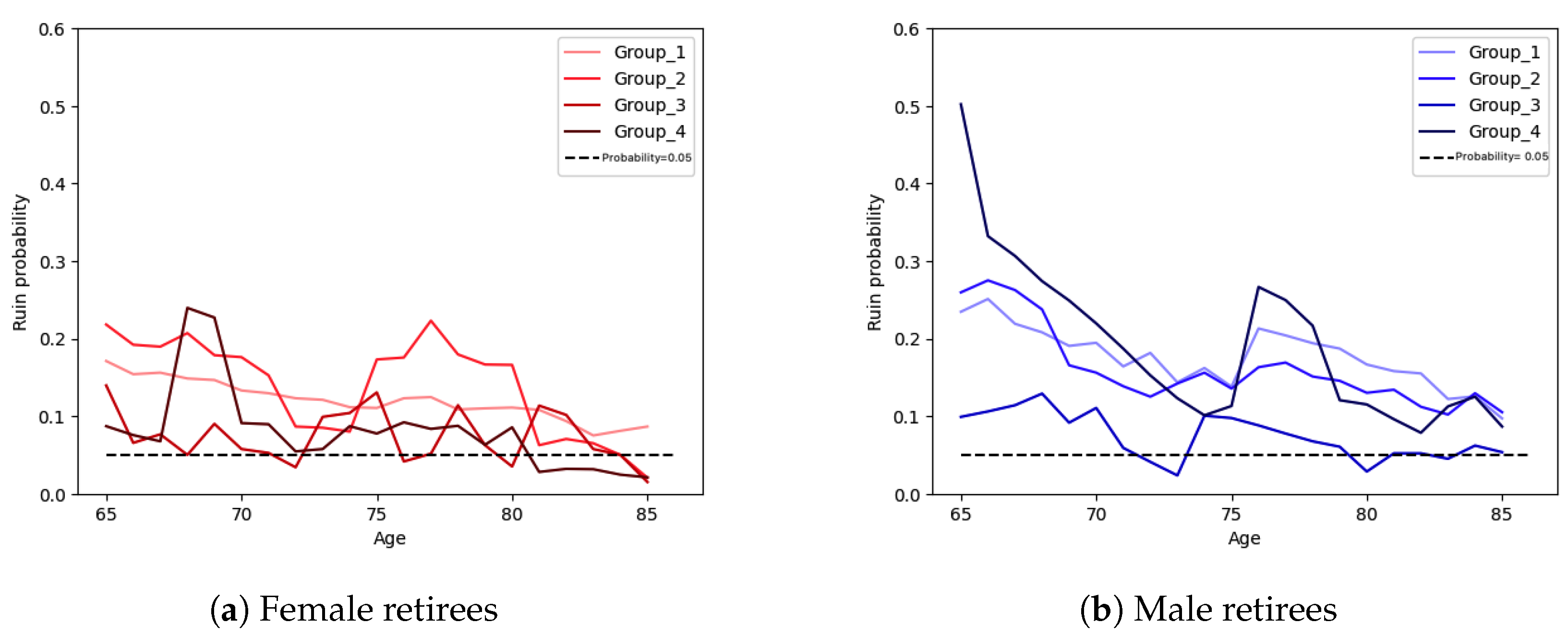
For deciding on which one of the two statistics, mean or median time, to rely on, we calculate the probabilities of ruin within the life expectancy of our retired clients for all groups of male and female retirees. Figure 9 displays the results as well as a horizontal line at $0.05$ for ease of comparison. We see there that the ruin probabilities are such that they support using the median for the time to exhaustion of funds instead of the mean. This is due to how we estimate the ruin probabilities (see Algorithm 2). It is consistent with the definition of percentiles and the most common percentile that is clearly interpreted is the median. Also, it can be seen that group 3 of male retirees have the lowest ruin probability within the life expectancy at all ages, while the ruin probabilities within the life expectancy for female retirees in groups 3 and 4 are the lowest ones. Lastly, we note that group 4 of male retirees have the highest ruin probabilities almost at all ages.

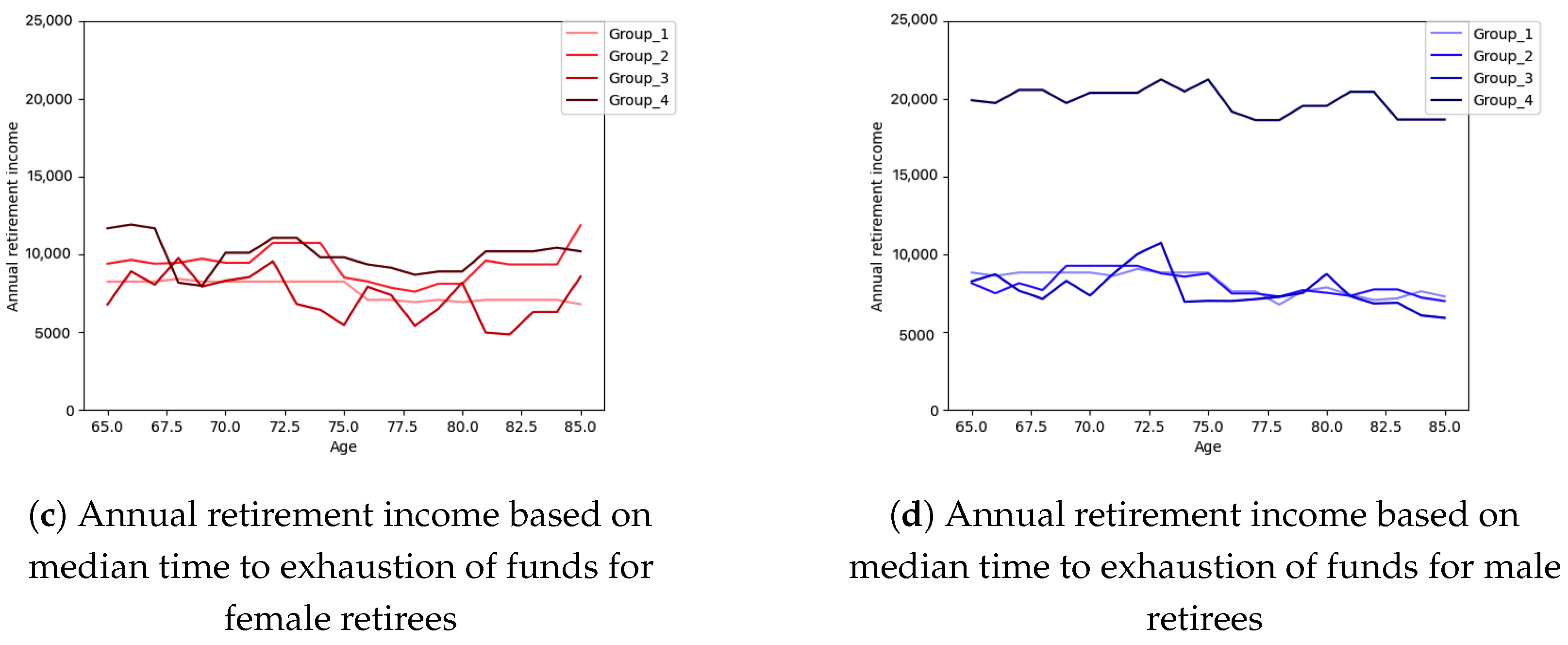
Figure 10 shows the annual retirement income based on mean and median time to exhaustion of funds for male and female retirees from age 65 to 85 and for all groups of risk tolerance, respectively. Because the median time to exhaustion of funds is greater than the mean time to exhaustion of funds at all ages and for all groups of risk tolerance, in Figure 10, we see that the annual retirement income based on mean time to exhaustion of funds are greater than the annual retirement income based on mean time to exhaustion of funds although the difference between them can be considered negligible. Group 4 of male and female retirees have the highest annual retirement incomes which can be more interesting when we look at the ruin probabilities in Figure 9 where the ruin probability for female retirees in group 4 is almost the lowest probability among other groups of female retirees and it can be due to the higher initial wealth that the retired clients in this group have.

In Figure 11, the mean and median deficit at ruin for female and male retirees in different groups of risk tolerance are shown. On the one hand, for the mean deficit at ruin, it is seen there that whenever ruin occurs, the deficit for group 4 of male retirees is much larger than for the other groups. This is a consequence of the pattern of their transactions which are shown in Figure 2. By looking at transactions in this figure, we can see that the average amount of withdrawals is roughly three times greater than the average amount of deposits for group 4 of male retirees which is the reason that in the case of ruin, the deficit for male retirees in group 4 is quite large compared to other groups. Among different groups of risk tolerance of female retirees, those in group 1 have the largest deficit at ruin which is again due to the pattern of their transactions which can be seen in Figure 2 that they have a much larger average of withdrawals in comparison with the average of deposits which eventually cause larger deficit at ruin. We note that although the average amount of deposits might be greater than the average of withdrawals in trades for some groups (such as group 4 of male retirees and group 1 of female retirees that are discussed), the less frequency of trades and high frequency of transactions leads to higher impact of transactions compared to trades in case of ruin and the mean deficit at ruin. On the other hand, it can be seen that the median deficit at ruin for all groups of female and male retirees is significantly lower than the mean at ruin. The median at ruin for all groups of both genders is around CAD 50,000 which by considering the annual retirement income that we obtained, we can conclude that is much more reliable compared to the mean deficit at ruin.

Lastly, in

Table 5. Withdrawal rates for male and female retirees and for all groups of risk tolerance.

Gender	Group 1	Group 2	Group 3	Group 4
Male	2.8%	2.7%	2.3%	4.6%
Female	2.1%	2.7%	2.2%	2.3%

, the withdrawal rates (as percentages of the initial wealth) based on median time to exhaustion of funds are shown for male and female retirees and all groups of risk tolerance. As seen in Table 5, group 4 of male retirees who are in the highest risk tolerance group has the highest withdrawal rate which is $4.6\%$ and group 1 of female retirees who are in the lowest risk tolerance group has the lowest withdrawal rates which is $2.1\%$.

Remark 1. 

In Finke et al. (2011), it is concluded that risk-tolerant clients, tend to withdraw more money. In this research, by segregating retirees by gender, we can enhance the findings of Finke et al. (2011) by suggesting that the assertion “risk-tolerant clients tend to withdraw more" might apply specifically to male clients.

Remark 2. 

Some studies, like those by Pfau (2011), Anarkulova et al. (2022), Saraogi (2022), and Raju and Saraogi (2024), deem the 4% rule risky, while others such as Finke et al. (2011) and Van Appel and Maré (2022) find it too conservative. Our analysis of the initial wealth and portfolio returns of our retired clients suggests that a 4.5% withdrawal rate maintains an acceptable risk level.

6. Conclusions

This research aims to help retirees afford post-retirement expenses and maintain their quality of life. We analyze data from over 4500 retirees to assess different investment and spending strategies. Our purpose is to provide insights to advise retirees on safe withdrawal practices, conservative approaches, and appropriate investment strategies based on their life stage. In this section, we discuss the results outlined in Section 5. We obtained the mean and the median time to exhaustion of funds and subsequently, the annual retirement income based on the mean and the median times. From Figure 8, it can be seen that the simulated data for time to exhaustion of funds, based on the mean and the median for all groups of male and female retirees does not show significant difference while both are considerably higher than the life expectancy. Although there is no significant difference between mean and median times, the ruin probabilities (see Figure 9) in life expectancy perfectly support the median time to ruin that is obtained, so for the time to ruin and consequently the annual retirement income, we rely on median time instead of the mean time. For the population that we study, the ruin probabilities within the retirees’ life expectancy are not low: in most cases exceeding 5% and for female and male retirees below 20% and 30%, respectively. In Figure 9, we can see that the ruin probability for males in group 4 at the age of 65 is pretty high, around $0.5$, which drops dramatically for following ages and this high ruin probability matches what we see in the plots related to median time to ruin in Figure 8 and the time to ruin for male retirees in group 4 that is even less than the life expectancy at age 65.

Male retirees in group 4 and female retirees in group 2 have the lowest time to exhaustion of funds at all ages and the highest ruin probabilities at almost all ages. Although we expect that the shortest time to ruin is associated with the highest annual retirement income, this is only the case for male retirees in group 4 of risk tolerance which is completely reasonable due to their initial wealth that is at least 30% higher than other groups of male retirees. Considering the highest initial wealth and the lowest time to ruin that male retirees in group 4 have, by looking at Figure 10, we can see that the highest annual retirement income, belongs to this group of retired clients. For female retirees in group 2, due to the lower initial wealth that they have, although their time to ruin is the shortest one among all groups of female retirees, they do not have the highest annual retirement income, while the female retirees in group 4 do, because of their highest initial wealth compared to other groups of male and female retirees.

In some research conducted in this area, such as Finke et al. (2011), it is found that the risk-tolerant clients tend to withdraw more which is exactly the case for male retirees in our research. In Finke et al. (2011), the authors do not take into account gender in their investigations of withdrawal rates and income, while in this paper we consider gender as an important factor. By separating the retirees based on their gender, we can refine the result in the mentioned paper by specifying that the statement “the risk-tolerant clients tend to withdraw more” might be true only for males.

In our study, 5%, 16%, 62%, and 17% of male retirees belong to groups 1 to 4, respectively. Across all groups, about 60% of male retirees have a ruin probability that is less than 10%, which is still a high probability within one’s life expectancy. For female retirees, 6%, 17%, 55%, and 22% belong to groups 1 to 4, respectively. In total, for about 80% of them, the ruin probability is less than 10%. About 60% and 80% of male and female retirees have time to ruin (exhaustion of funds) higher than the remaining time for their age to the maximum age (we consider the maximum age to be 110 here) which shows that they are withdrawing in a very safe way that might not be necessary. If we look at Table 5, we can see that the unnecessarily low withdrawal rates are around 2.5%, so it might be advisable for those retired clients who withdraw around 2.5%, by considering their risk tolerance group, to withdraw more.

We now address the question of what a safe withdrawal rate would be. In the literature, the 4% rule is considered risky in some research (for instance, see Anarkulova et al. 2022; Pfau 2011; Raju and Saraogi 2024; Saraogi 2022) and too low in others (for example, see Finke et al. 2011; Van Appel and Maré 2022). Given the initial wealth of our retired clients and the returns that their portfolios generate, our data suggests that a withdrawal rate of around 4.5% of the initial wealth will result in an acceptable ruin probability and time to ruin. Nevertheless, this corresponds to a yearly income of less than CAD 10,000 for most of the male and female retirees, which is obviously inadequate to meet expenses, while withdrawing around 4.5% leads to approximately CAD 20,000 annual retirement income for males in group 4.

Note that the amounts of initial wealth that we observe in our data (see Figure 7) are somewhat representative of the retirement savings of Canadians in general, see www.statcan.gc.ca, accessed on 1 September 2023. We note that in Canada the calculated annual retirement incomes are often supplemented by Old Age Security (OAS) and Canada Pension Plan (CPP). According to www.canada.ca-OAS (accessed on 1 September 2023) and www.canada.ca-CPP (accessed on 1 September 2023), these two governmental plans for retirees provide:

• OAS: Maximum monthly payments of CAD 698.60 for ages 65 to 74 and CAD 768.46 for 75 and over;
• CPP: Maximum monthly amounts of CAD 1306.57 and the monthly average amount is CAD 760.07 for retirement at age 65.

Therefore, OAS and CPP add total maximum annual payments of CAD 23,970.84 for ages 65 to 74 and CAD 24,798.84 for 75 and over for retirement at age 65. In particular, this can reduce significantly the ruin probabilities while extending the time to exhaustion of funds for Canadians. In conclusion, about CAD 24,000 to CAD 25,000 annually will be added to the annual retirement income for the average Canadian, which, although safe, still seems on the lower end for meeting daily expenses. As the final point, we note that according to www.statcan.gc.ca (accessed on 9 September 2023) the median after-tax of Canadian families and unattached individuals was CAD 68,400 in the year 2021 which is reasonably close to the annual retirement income that we estimate for our retired clients and it shows that our retirees are somehow representative of Canadians retirees.

Naturally, the model that we are proposing in this paper has certain limitations. Although it may be utilized for other datasets and countries, all simulation assumptions highly depend on the specific dataset which we are applying our methodology. For instance, the correlations between the frequencies and the amounts of deposits and withdrawals could be quite different for another dataset, regardless of whether it concerns a private company or a governmental agency. Thus, the outcome of the analysis might differ from what we observe in this research. In fact, all the parameters and distributions that are used in the simulations of the model need to be deduced carefully from the data at hand. Finally, one may extend our methodology further to pre-retirement savings while market shocks and long-term return on investments are also accounted for.

References

- Albrecher, Hansjörg, and Jef. L. Teugels. 2006. Exponential behavior in the presence of dependence in risk theory. Journal of Applied Probability 43: 257–73. [Google Scholar] [CrossRef]
- Albrecher, Hansjörg, Corina Constantinescu, and Stéphane Loisel. 2011. Explicit ruin formulas for models with dependence among risks. Insurance: Mathematics and Economics 48: 265–70. [Google Scholar] [CrossRef]
- Ali, Mukhtar M. 1987. Durbin-Watson and generalized Durbin-Watson tests for autocorrelations and randomness. Journal of Business & Economic Statistics 5: 195–203. [Google Scholar]
- Anarkulova, Aizhan, Scott Cederburg, Michael S. O’Doherty, and Richard W. Sias. 2022. The Safe Withdrawal Rate: Evidence from a Broad Sample of Developed Markets. Available online: https://ssrn.com/abstract=4227132 (accessed on 1 January 2024).
- Bengen, William P. 1994. Determining withdrawal rates using historical data. Journal of Financial Planning 7: 171–80. [Google Scholar]
- Blier-Wong, Christopher, Hélène Cossette, and Etienne Marceau. 2022. Collective risk models with FGM dependence. arXiv arXiv:2209.13543. [Google Scholar]
- Bouyé, Eric, Valdo Durrleman, Ashkan Nikeghbali, Gaël Riboulet, and Thierry Roncalli. 2000. Copulas for Finance—A Reading Guide and Some Applications. Available online: https://ssrn.com/abstract=1032533 (accessed on 1 September 2023).
- Bregman, Yuliya, and Claudia Klüppelberg. 2005. Ruin estimation in multivariate models with clayton dependence structure. Scandinavian Actuarial Journal 2005: 462–80. [Google Scholar] [CrossRef]
- Chadjiconstantinidis, Stathis, and Spyridon Vrontos. 2014. On a renewal risk process with dependence under a Farlie–Gumbel–Morgenstern copula. Scandinavian Actuarial Journal 2014: 125–58. [Google Scholar] [CrossRef]
- Cossette, Helene, Etienne Marceau, and Fouad Marri. 2008. On the compound Poisson risk model with dependence based on a generalized Farlie–Gumbel–Morgenstern copula. Insurance: Mathematics and Economics 43: 444–55. [Google Scholar] [CrossRef]
- Cross, George R., and A. K. Jain. 1982. Measurement of clustering tendency. In Theory and Application of Digital Control. Amsterdam: Elsevier, pp. 315–20. [Google Scholar]
- Denuit, Michel, Jan Dhaene, Marc Goovaerts, and Rob Kaas. 2006. Actuarial Theory for Dependent Risks: Measures, Orders and Models. Hoboken: John Wiley & Sons. [Google Scholar]
- Finke, Michael S., Wade D. Pfau, and Duncan Williams. 2011. Spending Flexibility and Safe Withdrawal Rates. Available online: https://www.financialplanningassociation.org/sites/default/files/2020-05/3%20Spending%20Flexibility%20and%20Safe%20Withdrawal%20Rates.pdf (accessed on 1 September 2023).
- Frees, Edward W., and Emiliano A. Valdez. 1998. Understanding relationships using copulas. North American Actuarial Journal 2: 1–25. [Google Scholar] [CrossRef]
- Gastner, Michael T. 2005. Spatial Distributions: Density-Equalizing Map Projections, Facility Location, and Two-Dimensional Networks. Ann Arbor: University of Michigan. [Google Scholar]
- Guan, Lihong, and Xiaohong Wang. 2023. Ruin analysis on a new risk model with stochastic premiums and dependence based on time series for count random variables. Entropy 25: 698. [Google Scholar] [CrossRef]
- Hopkins, Brian, and John Gordon Skellam. 1954. A new method for determining the type of distribution of plant individuals. Annals of Botany 18: 213–27. [Google Scholar] [CrossRef]
- Joe, Harry. 1997. Multivariate Models and Multivariate Dependence Concepts. Boca Raton: CRC Press. [Google Scholar]
- Kassambara, Alboukadel. 2017. Practical Guide to Cluster Analysis in R: Unsupervised Machine Learning. Sthda: CreateSpace Independent Publishing Platform, vol. 1. [Google Scholar]
- Labbé, Chantal, and Kristina P. Sendova. 2009. The expected discounted penalty function under a risk model with stochastic income. Applied Mathematics and Computation 215: 1852–67. [Google Scholar] [CrossRef]
- McNeil, Alexander J., Rüdiger Frey, and Paul Embrechts. 2015. Quantitative Risk management: Concepts, Techniques and Tools-Revised Edition. Princeton: Princeton University Press. [Google Scholar]
- Milevsky, Moshe A., Kristen S. Moore, and Virginia R. Young. 2006. Asset allocation and annuity-purchase strategies to minimize the probability of financial ruin. Mathematical Finance 16: 647–71. [Google Scholar] [CrossRef]
- Moore, Kristen S., and Virginia R. Young. 2006. Optimal and simple, nearly optimal rules for minimizing the probability of financial ruin in retirement. North American Actuarial Journal 10: 145–61. [Google Scholar] [CrossRef]
- Nelsen, Roger B. 2007. An Introduction to Copulas. Berlin/Heidelberg: Springer Science & Business Media. [Google Scholar]
- Pfau, Wade D. 2011. An international perspective on safe withdrawal rates from Retirement Savings: The Demise of the 4 Percent Rule? Journal of Financial Planning 15: 52–61. [Google Scholar]
- Raju, Rajan, and Ravi Saraogi. 2024. Balancing Acts: Safe Withdrawal Rates in the Indian Context. Available at SSRN. Available online: https://papers.ssrn.com/sol3/papers.cfm?abstract_id=4697720 (accessed on 30 February 2024).
- Rousseeuw, Peter J. 1987. Silhouettes: A graphical aid to the interpretation and validation of cluster analysis. Journal of Computational and Applied Mathematics 20: 53–65. [Google Scholar] [CrossRef]
- Saraogi, Ravi. 2022. Computing the Safe Withdrawal Rate for a Retirement Portfolio in India. Available online: https://papers.ssrn.com/sol3/papers.cfm?abstract_id=4216077 (accessed on 30 February 2024).
- Schabort, Kilian Petika. 2022. Sequence of Return Risk in South African Post-Retirement Portfolios: The Effectiveness of Volatility-Focused Asset Allocation Strategies to Address Sequence and Associated Risks. Available online: http://hdl.handle.net/11427/36552 (accessed on 1 November 2023).
- Stocker, Alan. 2023. The effect of defined benefit pensions on income survivability and ‘safe’withdrawal rates in retirement. Social Science Research Network 12. [Google Scholar] [CrossRef]
- Van Appel, Vaughan, and Eben Maré. 2022. Determining safe retirement withdrawal rates using forward-looking distributions. South African Journal of Science 118: 1–7. [Google Scholar] [CrossRef]
- Van Appel, Vaughan, Eben Maré, and Andries Van Niekerk. 2021. Quantitative guidelines for retiring (more safely) in South Africa. South African Actuarial Journal 21: 75–91. [Google Scholar] [CrossRef]
- Vidmar, Matija. 2018. Ruin under stochastic dependence between premium and claim arrivals. Scandinavian Actuarial Journal 2018: 505–13. [Google Scholar] [CrossRef]
- Wang, Shaun. 1998. Aggregation of correlated risk portfolios: Models and algorithms. In Proceedings of the Casualty Actuarial Society. Arlington: Citeseer. Available online: https://www.casact.org/sites/default/files/database/proceed_proceed98_980848.pdf (accessed on 1 January 2024).
- Xie, Jie-Hua, and Wei Zou. 2013. On a risk model with random incomes and dependence between claim sizes and claim intervals. Indagationes Mathematicae 24: 557–80. [Google Scholar] [CrossRef]
- Zhang, Zhimin, and Hu Yang. 2010. On a risk model with stochastic premiums income and dependence between income and loss. Journal of Computational and Applied Mathematics 234: 44–57. [Google Scholar] [CrossRef]
Figure 1.
Average annual number of deposits and average annual number of withdrawals.
Figure 2.
Average amount of deposits and withdrawals.
Figure 3.
Correlation between the annual frequencies of deposits and withdrawals.
Figure 4.
Correlation between the total amount of annual deposits and withdrawals.
Figure 5.
Histograms of non-parametric densities for group 3 of male retirees.
Figure 6.
Histogram and non-parametric fitted density curve of distribution for group 3 of female retirees.
Figure 7.
Retirees’ initial wealth for female and male retirees for ages 65 to 85 and different groups of risk tolerance.
Figure 8.
Mean and median time to exhaustion of funds for female and male retirees for ages 65 to 85 and different groups of risk tolerance.
Figure 9.
Ruin probabilities during the life expectancy for female and male retirees for ages 65 to 85 and different groups of risk tolerance.
Figure 10.
Annual retirement income based on mean and median time to exhaustion of funds for female and male retirees for ages 65 to 85 and different groups of risk tolerance.
Figure 11.
Mean and median deficit at (financial) ruin for female and male retirees for ages 65 to 85 and different groups of risk tolerance.