Optimal Time to Enter a Retirement Village

Abstract

We consider the financial planning problem of a retiree wishing to enter a retirement village at a future uncertain date. The date of entry is determined by the retiree’s utility and bequest maximisation problem within the context of uncertain future health states. In addition, the retiree must choose optimal consumption, investment, bequest and purchase of insurance products prior to their full annuitisation on entry to the retirement village. A hyperbolic absolute risk-aversion (HARA) utility function is used to allow necessary consumption for basic living and medical costs. The retirement village will typically require an initial deposit upon entry. This threshold wealth requirement leads to exercising the replication of an American put option at the uncertain stopping time. From our numerical results, active insurance and annuity markets are shown to be a critical aspect in retirement planning.

1. Introduction

With the reduced mortality rate, life expectancy is continuing to increase globally [1]. In the next 40–50 years, the percentage of people aged over 60 years will nearly double all over the world. People are predicted to have longer lives and extended retirement living.

Australia has one of the longest life expectancies in the world, that is, 79.7 years for males and 84.2 years for females [2]. With the growing ageing population, Australia is now facing a profound ageing problem. The potential impact includes economy stagnation, high demand for pensions and increased aged care spending, which has caught Australian Government’s attention [3].

As reported by the Australia Institute of Health and Welfare [4], 28.31% of the population aged 65 or over receive aged care services. This requires recurrent annual expenditure of more than A$13 billion for the Australian federal, state and territory governments. Almost 70% of the total spending on aged care is allocated to residential aged care services, that is, aged care homes [5]. The increasing demand for aged care has become a burden for the Australian government. Hence, improving wellness during retirement living has become a more profound topic.

For the growing senior population, retirement villages which are linked with “active ageing” and “community support” present an alternative high-quality retirement living option. From Glass and Skinner [6], a retirement village or retirement community can be defined as an organised residential place with a certain level of service for a voluntary age-specified retired or partially retired person. The retirement village should provide its residents with shared activities and facilities in a community that offers secured living [7].

In the United States, a retirement village is usually called a retirement community. According to the size, scale, location, and facilities and activities provided, the retirement community can be classified into different categories, such as senior apartments, continuing-care retirement communities, leisure-oriented retirement communities, congregate housing, etc. [6]. In the United Kingdom (UK), the retirement village is now growing as a new growing long-term residential option for retirees [7].

It is well documented in the literature that residing in a retirement village can improve well-being. Factors that contribute to well-being include community facilities, accessibility features and 24-h emergency assistance [8], social contact [9,10], living independence [11] and organised group activity and exercise [12].

The Property Council of Australia [13] states that currently over 177,000 seniors aged 65 and over (i.e., only 5% of the total number) reside in an Australian retirement village. However, as stated by the Australian Bureau of Statistics [14], males have recently been stated to close the life expectancy gap. This prevailing tendency implies that retirees are expected to live a longer time as a part of a couple. As an alternative retirement living option for a spouse, retirement villages would attract more demand [6].

Optimal strategies have been widely studied for a variety of financial problems appearing in the literature. Merton [15,16] developed a well-known optimal asset allocation and consumption model for an investor with a fixed lifetime. In the model, utility is measured by a constant relative risk-aversion (CRRA) function and is maximised by the investor to determine her optimal strategy. Ding et al. [17] used put option replication to create a wealth threshold in Merton’s model to allow for a luxury bequest. Noting the conclusion from Yaari [18] that investors benefit from a life annuity, Merton’s model was extended in [19] by Richard in which investors were assumed to have a stochastic lifetime and access to the purchase of insurance products, that is, life insurance and life annuities.

Within the framework of Merton’s model, Milevsky and Young [20] studied an optimal stopping problem for investors seeking a once-and-for-all annuitisation. Kingston and Thorp [21] extended the work of [20] to the more general case of hyperbolic absolute risk-aversion (HARA) utility. Dybvig and Liu [22], and Barucci and Marazzina [23] investigate the lifetime asset allocation problem for an investor who have stochastic labor income and can choose her retirement date.

Health status is another aspect which impacts on financial decision. Rosen and Wu [24] showed that self-rated health status is a profound indicator for portfolio choice. Bernheim et al. [25] studied the circumstances under which health status can initiate bequest motives. Edwards [26] explored the link between health status and portfolio selection. Specifically, in [26], the decline of financial risk observed after investors’ retirement is partially explained by investors’ health risk which usually increases along with age. Furthermore, the existence of medical costs associated with their health risk can vary retirees’ financial strategy. Retirees who pay out-of-pocket medical costs consequently have less wealth [27] and tend to save more [28].

This arising ageing problem provided us with the motivation to develop a life-cycle model involving retirement living choices while considering asset allocation, consumption, bequests and insurance purchase, thus contributing to our understanding of the optimal financial behaviour of the ageing. In our model, retirees are found to have an increasing proportion of wealth invested in risky assets in line with their increasing age, when there is a wealth requirement threshold to enter a retirement village. This increasing proportion trend during retirement is also stated in Kingston and Fisher [29], Ding et al. [17] and Pfau and Kitces [30]. By allowing for dynamic health states, our model can be more suitable for the ageing problem.

In this paper, we study the retirees’ optimal strategy models for different cases in Section 2. Numerical demonstrations (and parameters) are presented and discussed in Section 3 and Section 4 and are followed by the conclusion in Section 5.

2. Model and Method

We assume that risky assets available in the market follow the geometric Brownian motion:

$$\begin{array}{c}d{X}_t=\alpha X_{t}dt+\sigma X_{t}d{B}_t,\end{array}$$

(1)

where $\alpha$ and $\sigma$ are the expected return rate and volatility of the risky assets $X_t$ and $B_t$ is the standard Brownian motion.

In this paper, we use a HARA utility function for consumption, that is,

$$\begin{array}{c}\hfill U_1(C)=\frac{{(C-h)}^{\gamma }}{\gamma },\end{array}$$

where C is consumption, h is consumption of necessities for basic living (not including medical costs) and $\gamma$ is a constant that reflects the individual’s level of risk aversion.

Drawing on Haberman and Pitacco [31] and the theory of continuous-time Markov chains1, we assume the retiree’s health status is stochastic and is modelled by a continuous Markov chain process with the transition matrix shown as follows

$$\begin{array}{c}\hfill \mathbf{Q}=\left(\begin{array}{cc}{q}_{11}& q_{12}\\ q_{21}& q_{22}\end{array}\right),\end{array}$$

(2)

where $q_{11}$ is the intensity of staying in a healthy state, $q_{12}$ is the intensity of becoming sick from a healthy state, $q_{21}$ is the intensity of recovery from a sick state to a healthy state and $q_{22}$ is the intensity of staying in a sick state. Here state 1 represents a healthy condition and state 2 represents a sick condition. For the homogeneity case, we have the transition probability of staying healthy, being sick from a healthy state, recovery from being sick to a healthy state and staying in a sick state, that is, ${\tilde{P}}_{11}$, ${\tilde{P}}_{12}$, ${\tilde{P}}_{21}$ and ${\tilde{P}}_{22}$

$$\begin{array}{cc}\hfill {\tilde{P}}_{11}(t,T)& =\frac{1}{q_{12}+q_{21}}[q_{21}+q_{12}{e}^{-(q_{12}+q_{21})(T-t)}]\hfill \end{array}$$

(3)

$$\begin{array}{cc}\hfill {\tilde{P}}_{12}(t,T)& =1-{\tilde{P}}_{11}(t,T)\hfill \end{array}$$

(4)

$$\begin{array}{cc}\hfill {\tilde{P}}_{21}(t,T)& =1-{\tilde{P}}_{22}(t,T)\hfill \end{array}$$

(5)

$$\begin{array}{cc}\hfill {\tilde{P}}_{22}(t,T)& =\frac{1}{q_{12}+q_{21}}[q_{12}+q_{21}{e}^{-(q_{12}+q_{21})(T-t)}],\hfill \end{array}$$

(6)

where ${\tilde{P}}_{ij}(t,T)$ is the transition probability from state i to state j with time interval $(t,T)$.

In our model, a known distribution is assumed to describe the lifetime of retirees. The density function of mortality $f_x(t)$ is defined as follows,

$$\begin{array}{c}\hfill f_x(t)=\mu (t)·S(t),\end{array}$$

where $\mu (t)$ is the force of mortality and $S(t)$ is the survival probability.

Further, retirees are assumed to have short-sighted or myopic vision about their future health state. That is, although their health state can continually change, reflected in the modelling above, our myopic agents make their plans assuming their current health state will continue indefinitely into the future. We make this assumption to reduce the complexity of our already complex model. Allowing agents to plan their future aware of future health changes is recognised as a mathematically difficult problem [33], and we leave this task for future research. Unlike Milevsky and Young [20], we do not explore asymmetric information between insured/annuitant and insurer, and so we assume insurers share the retirees’ myopia.

With an assumed two-state health stochastic process $\{H(s),t\le s\le \tau \}$, the presence of myopic retirees making financial plans at some time t implies

$$\begin{array}{cc}\hfill \mu (s)& =\left\{\begin{array}{cc}{\mu }_1(s),\hfill & H(t)=h_t=1,t\le s\le \tau \hfill \\ {\mu }_2(s),\hfill & H(t)=h_t=2,t\le s\le \tau \hfill \end{array}\right.\hfill \end{array}$$

(7)

with its corresponding $S(s)$, and so myopia implies $H(s)=h_t,t\le s\le \tau$, for some deterministic maximum age $\tau$, and where $h_t$ is the realisation of the individual’s current health state at time t, ${\mu }_i(s)$ and its corresponding $S_i(s)$ are the future force of mortality and survival probability at time s for health state i. In this paper, state 1 represents the healthy state and state 2 represents the sick state. Hence, ${\mu }_1(s)\le {\mu }_2(s)$ and $S_1(s)\ge S_2(2)$.

2.1. Case 1: No Bequest and Incomplete Insurance Market

In Australia, several types of housing are offered by retirement villages. One common type is the serviced apartment offered by a lease contract. These apartment-type residential options for seniors can also be found in other countries, such as in the UK and the United States. For this case, the retirees rent the apartment on a pay-as-you-go basis to move into a retirement village. According to [34], an owner-occupied house can be treated as a bequest. So, in the case of leased serviced apartments, as retirees do not own the residential property in the retirement village, some of these retirees will have no bequest motive. Focusing on such retirees, we further assume they have no access to insurance markets prior to their full annuitisation on their entry to the retirement village—with no bequest motive they have no interest in life insurance and to thwart their interest in annuitisation prior to entering a retirement village is an important consideration given the widespread incompleteness of annuity markets worldwide [35].

Meanwhile, retirees are assumed to maximise their utilities by consumption and investment before the optimal time $\tilde{\tau }$, that is, the chosen optimal time to enter retirement villages. At time $\tilde{\tau }$, retirees without a bequest motive would use all their remaining wealth to purchase a life annuity at the time they enter retirement villages.

Therefore, following [19,20], the value function of this optimal problem is as follows:

$$\begin{array}{cc}\hfill V& =\underset{\pi ,C,\tilde{\tau }}{max}E\left\{{\int }_t^{\tilde{\tau }}\frac{S(s)}{S(t)}{e}^{-\rho (s-t)}{U}_1(C(s))ds+{\int }_{\tilde{\tau }}^{\tau }\frac{S(s)}{S(t)}{e}^{-\rho (s-t)}{U}_1\left(\frac{W(\tilde{\tau })}{{\overline{a}}_{\tilde{\tau }}}\right)ds|H(s)=h_t,t\le s\le \tau \right\}\hfill \end{array}$$

(8)

$$\begin{array}{cc}& =\underset{\pi ,C,\tilde{\tau }}{max}E\left\{{\int }_t^{\tilde{\tau }}\frac{S(s)}{S(t)}{e}^{-\rho (s-t)}{U}_1(C(s))ds+e^{-\rho (\tilde{\tau }-t)}\frac{S(\tilde{\tau })}{S(t)}{\overline{a}}_{\tilde{\tau }}{U}_1\left(\frac{W(\tilde{\tau })}{{\overline{a}}_{\tilde{\tau }}}\right)|H(s)=h_t,t\le s\le \tau \right\},\hfill \end{array}$$

(9)

with the wealth dynamics as

$$\begin{array}{c}\hfill dW(t)=(rW(t)-D(t)W(t)-C(t)+(\alpha -r)\pi (t)W(t))dt+\sigma \pi (t)W(t)d{B}_t,\end{array}$$

where t is the starting age, $\pi (t)$ is the proportion of total wealth invested in risky assets, ${\overline{a}}_t={\int }_t^{\tau }\frac{S(s)}{S(t)}{e}^{-\rho (s-t)}ds$ is the annuity function and $D(t)$ is the medical cost represented by a percentage of wealth. As with the force of mortality and survival rate,

$$\begin{array}{c}\hfill D(s)=D_{h_t}(s),t\le s\le \tau .\end{array}$$

(10)

For simplicity, we set the time preference rate equal to the risk free rate, $\rho =r$.

As retirees in our model are assumed to be myopic with respect to their future health states, they develop their financial strategies ignoring future health dynamics. In another words, although retirees’ health states can switch between different regimes, the view of a myopic retiree still will be limited to his or her current health condition and this is the reason for not including transition probabilities in our HJB equations. While our approach handles the regime switching environment within which it is set, we point to [36] as a reference for the generalised setting for regime switching environments.

From Milevsky and Young [20], and Kingston and Thorp [21], the optimal stopping time $\tilde{\tau }$ has been proven to be deterministic for CRRA utility and HARA utility. Based on Milevsky and Young [20], and Øksendal [37], the variational inequality is shown as follows,

$$\begin{array}{cc}\hfill (\rho +\mu (t))V& \ge V_t+(r-D(t))W(t)V_W+\underset{c}{max}[U_1(C(t))-C(t)V_W]\hfill \\ & +\underset{\pi }{max}[(\alpha -r)\pi W(t)V_W+\frac{1}{2}{\sigma }^2{\pi }^{2}W{(t)}^2{V}_{WW}],t\in [0,\tilde{\tau }]\hfill \end{array}$$

(11)

and

$$\begin{array}{c}\hfill V\ge {\overline{a}}_t{U}_1(\frac{W(t)}{{\overline{a}}_t}),t\in (\tilde{\tau },\tau ).\end{array}$$

(12)

The form of solution for V is assumed to be

$$\begin{array}{c}\hfill V=\frac{1}{\gamma }{(W(t)-\widehat{W}(t))}^{\gamma }a{(t)}^{1-\gamma },\end{array}$$

(13)

where

$$\begin{array}{c}\hfill \widehat{W}(t)=\frac{h}{r-D(t)}(1-e^{-(r-D(t))(\tau -t)})\end{array}$$

is the ‘floor’ or ‘protected’ wealth, and $r-D(t)$ reflects the continuous compounding rate of interest to give the retirees an income stream covering health costs up to the maximum possible age $\tau$. Such protection is needed as they are assumed to have no access to insurance markets prior to entry to the retirement village. Further note that $a(t)$ is health state dependent.

We also write $\tilde{W}(t)=W(t)-\widehat{W}(t)$ as the difference between wealth and protected wealth which is known as ‘surplus’ wealth.

The derivatives of the value function are then

$$\begin{array}{ccc}& \hfill V_t& =\frac{1-\gamma }{\gamma }\tilde{W}{(t)}^{\gamma }a{(t)}^{-\gamma }{a}^{\prime }(t)+\tilde{W}{(t)}^{\gamma -1}a{(t)}^{1-\gamma }h,\hfill \\ & \hfill V_W& =\tilde{W}{(t)}^{\gamma -1}a{(t)}^{1-\gamma },\hfill \\ (14)& \mathrm{and}\hfill & \hfill V_{WW}& =(\gamma -1)\tilde{W}{(t)}^{\gamma -2}a{(t)}^{1-\gamma }.\hfill \end{array}$$

Following Milevsky and Young [20], and Kingston and Thorp [21], we can use the first order derivative condition of Equation (11) to show that the optimal consumption $C^{*}(t)$ and optimal proportion invested in risky assets are

$$\begin{array}{c}{C}^{*}(t)=\tilde{W}(t)a{(t)}^{-1}+h,\hfill \\ (15)& {\pi }^{*}(t)=\frac{\alpha -r}{{\sigma }^2(1-\gamma )}\frac{\tilde{W}(t)}{W(t)}\hfill \end{array}$$

and $C^{*}(t)$ depends on the current health state.

We substitute Equations (13)–(15) into (11) and (12): for $t\le \tilde{\tau }$, we have

$$\begin{array}{c}\hfill -1\ge a^{\prime }(t)+\frac{1}{1-\gamma }\left[\gamma r-\gamma D(t)-\rho -\mu (t)+\frac{1}{2}\frac{{(\alpha -r)}^2\gamma }{{\sigma }^2(1-\gamma )}\right]a(t),t\in [0,\tilde{\tau }],\end{array}$$

(16)

while for $t>\tilde{\tau }$, we have

$$\begin{array}{c}\hfill a(t)\ge {\overline{a}}_t,t\in (\tilde{\tau },\tau ).\end{array}$$

(17)

We adopt the hypothesis from Milevsky and Young [20] which assumes the time before full annuitisation is of the form $(0,\tilde{\tau })$. With this hypothesis, $\tilde{\tau }$ is set to be deterministic and we write $\varphi (t)$ as the solution of Equations (16) and (17) and let ${\eta }_1(t)=\frac{1}{1-\gamma }\left[\gamma r-\gamma D(t)-\rho -\mu (t)+\frac{1}{2}\frac{{(\alpha -r)}^2\gamma }{{\sigma }^2(1-\gamma )}\right]$. Hence, for $t\le \tilde{\tau }$, we have

$$\begin{array}{c}\hfill -1={\varphi }^{\prime }(t)+{\eta }_1(t)\varphi (t).\end{array}$$

(18)

Multiplying equation (18) by $e^{{\int }_0^t{\eta }_1(u)du}$, the equation can be shown as

$$\begin{array}{c}\hfill -e^{{\int }_0^t{\eta }_1(u)du}={\varphi }^{\prime }(t)e^{{\int }_0^t{\eta }_1(u)du}+{\eta }_1(t)\varphi (t)e^{{\int }_0^t{\eta }_1(u)du}.\end{array}$$

(19)

Integrating (19) from t to $\tilde{\tau }$, we can have

$$\begin{array}{c}\hfill {\int }_t^{\tilde{\tau }}-e^{{\int }_0^s{\eta }_1(u)du}ds={\left[\varphi (s)e^{{\int }_0^s{\eta }_1(u)du}\right]}_t^{\tilde{\tau }}\end{array}$$

and

$$\begin{array}{c}\hfill \varphi (t)={\overline{a}}_{\tilde{\tau }}{e}^{{\int }_t^{\tilde{\tau }}{\eta }_1(u)du}+{\int }_t^{\tilde{\tau }}{e}^{{\int }_t^s{\eta }_1(u)du}ds.\end{array}$$

(20)

For $t>\tilde{\tau }$, the solution $\varphi$ is

$$\begin{array}{c}\hfill \varphi (t)={\overline{a}}_{\tilde{\tau }}.\end{array}$$

We re-write $\varphi (t)$ as $\varphi (t,\tilde{\tau })$, as it contains both t and $\tilde{\tau }$.

To find the optimal stopping time, we can differentiate the value function (13) with respect to $\tilde{\tau }$,

$$\frac{\partial V}{\partial \tilde{\tau }}=\frac{1-\gamma }{\gamma }{W}^{\gamma }(t){\varphi }^{-\gamma }(t,\tilde{\tau })\frac{\partial \varphi (t,\tilde{\tau })}{\partial \tilde{\tau }},$$

and noting $\partial {\overline{a}}_{\tilde{\tau }}/\partial \tilde{\tau }=(\mu (\tilde{\tau })+\rho ){\overline{a}}_{\tilde{\tau }}-1$ and $\partial \varphi (t,\tilde{\tau })/\partial \tilde{\tau }=[(\mu (\tilde{\tau })+\rho ){\overline{a}}_{\tilde{\tau }}]e^{{\int }_t^{\tilde{\tau }}{\eta }_1(u)du}+{\overline{a}}_{\tilde{\tau }}{e}^{{\int }_t^{\tilde{\tau }}{\eta }_1(u)du}{\eta }_1(\tilde{\tau })$, with $W(t)$, $\varphi (t)$ and ${\overline{a}}_{\tilde{\tau }}$ always positive, then

$$\frac{\partial V}{\partial \tilde{\tau }}\propto \mu (\tilde{\tau })+\rho +{\eta }_1(\tilde{\tau })$$

and the optimal stopping time is given when this expression is zero.

2.2. Case 2: With Bequest and Complete Insurance Market

The most common housing type offered by retirement villages in Australia is the resident-funded unit. Retirees need to purchase a licence to reside in the retirement village and can sell the licence when they exit. This type of agreement is similar to a purchase in the real-estate market. Retirees who have a licence to live in a resident-funded unit can be regarded as house owners. Similarly, in the UK, retirees can purchase retirement housing on a leasehold basis2 or as a property owner. In the United States, it is also common for retirees to purchase properties in leisure-oriented retirement communities for retirement living. Following the assumption by [34]—that the owner-occupied house can be treated as a bequest—we can assume that those retirees have bequest motives and access to the insurance market prior to full annuitisation.

In this case, retirees are assumed to have bequest motives from time t to $\tilde{\tau }$. We use a power utility function for the bequest motive $U_2$, that is

$$\begin{array}{c}\hfill U_2(L(t))=m{(t)}^{1-\gamma }\frac{L{(t)}^{\gamma }}{\gamma },\end{array}$$

where $L(t)$ is the legacy amount and, following the argument in [38], with $m(t)=\frac{2}{3}{\int }_t^{\tau }{e}^{-r(u-t)}du$. In our calculation, we use $\tau$ to represent the deterministic maximum age.

We also assume that insurance products, that is, life insurance and annuities, are available in the market. Before the optimal time to enter a retirement village $\tilde{\tau }$, retirees use consumption, bequests and the purchase of insurance products to maximise their utility. From Richard [19], the insurance premium is related to $L(t)$ and wealth $W_t$ and given by3

$$\begin{array}{c}\hfill P(t)=\mu (t)[L(t)-W(t)]\end{array}$$

and where both $P(t)$ and $L(t)$ depend on the current health state.

At time $\tilde{\tau }$, retirees split their wealth into two parts: $\upsilon W_{\tilde{\tau }}$ and $(1-\upsilon )W_{\tilde{\tau }}$. The first part, $\upsilon W_{\tilde{\tau }}$, is used to purchase lifetime annuity products, with this being similar to the behaviour of retirees without a bequest motive. The second part, $(1-\upsilon )W_{\tilde{\tau }}$, reflects their altruism, with this sum to be delivered to their heirs at time $\tilde{\tau }$ as an inter vivos transfer. Hence, the value function is

$$\begin{array}{cc}\hfill V& =\underset{\pi ,C,L,\tilde{\tau }}{max}E\{{\int }_t^{\tilde{\tau }}\frac{S(s)}{S(t)}{e}^{-\rho (s-t)}\left[U_1(C(s))+\mu (s)U_2(L(s))\right]ds\hfill \\ & +{\int }_{\tilde{\tau }}^{\tau }\frac{S(s)}{S(t)}{e}^{-\rho (s-t)}{U}_1(\frac{\upsilon W(\tilde{\tau })}{{\overline{a}}_{\tilde{\tau }}})ds+\frac{S(\tilde{\tau })}{S(t)}{e}^{-\rho (\tilde{\tau }-t)}{U}_2((1-\upsilon )W(\tilde{\tau }))|H(s)=h_t,t\le s\le \tau \}\hfill \\ & =\underset{\pi ,C,L,\tilde{\tau }}{max}E\{{\int }_t^{\tilde{\tau }}\frac{S(s)}{S(t)}{e}^{-\rho (s-t)}\left[U_1(C(s))+\mu (s)U_2(L(s))\right]ds+e^{-\rho (\tilde{\tau }-t)}\frac{S(\tilde{\tau })}{S(t)}{\overline{a}}_{\tilde{\tau }}{U}_1(\frac{\upsilon W(\tilde{\tau })}{{\overline{a}}_{\tilde{\tau }}})\hfill \\ & +\frac{S(\tilde{\tau })}{S(t)}{e}^{-\rho (\tilde{\tau }-t)}{U}_2((1-\upsilon )W(\tilde{\tau }))|H(s)=h_t,t\le s\le \tau \}\hfill \end{array}$$

with the wealth dynamics

$$\begin{array}{c}\hfill dW(t)=(rW(t)-D(t)W(t)-C(t)+(\alpha -r)\pi (t)W(t)-P(t))dt+\sigma \pi (t)W(t)d{B}_t.\end{array}$$

The variational inequality is then shown as

$$\begin{array}{cc}\hfill (\rho +\mu (t))V& \ge V_t+rW{V}_W-P(t)V_W+\underset{C,L}{max}[U_1(C(t))+\mu (t)U_2(L(t))-C(t)V_W]\hfill \\ (21)& & +\underset{\pi }{max}[(\alpha -r)\pi W(t)V_W+\frac{1}{2}{\sigma }^2{\pi }^{2}W{(t)}^2{V}_{WW}],t\in [0,\tilde{\tau }]\hfill \end{array}$$

and

$$\begin{array}{c}\hfill V\ge \frac{{(\upsilon \frac{W(t)}{{\overline{a}}_{\tilde{\tau }}})}^{\gamma }}{\gamma }{\overline{a}}_{\tilde{\tau }}+\frac{{((1-\upsilon )W(t))}^{\gamma }m(t)}{\gamma },t\in (\tilde{\tau },\tau ).\end{array}$$

(22)

Similar to the case in Section 2.1, we have

$$\begin{array}{c}\hfill V=\frac{1}{\gamma }{(W(t)-\widehat{W}(t))}^{\gamma }a{(t)}^{1-\gamma },\end{array}$$

where

$$\begin{array}{c}\hfill \widehat{W}(t)=h{\int }_t^{\tau }\frac{S(s)}{S(t)}{e}^{-(r-D(t))(s-t)}ds.\end{array}$$

For the time $t\le \tilde{\tau }$, the value function reduces to Richard’s model [19] in which the optimal consumption $C^{*}(t)$, optimal legacy amount $L^{*}(t)$, optimal proportion invested in risky assets ${\pi }^{*}(t)$ and optimal insurance premium $P^{*}(t)$ are shown as follows

$$\begin{array}{cc}\hfill C^{*}(t)& =\tilde{W}(t)a{(t)}^{-1}+h,\hfill \\ \hfill L^{*}(t)& =m(t)\tilde{W}(t)a{(t)}^{-1},\hfill \\ \hfill {\pi }^{*}(t)& =\frac{\alpha -r}{{\sigma }^2(1-\gamma )}\frac{\tilde{W}(t)}{W(t)},\hfill \\ \hfill P^{*}(t)& =(L^{*}(t)-W(t))\mu (t)\hfill \\ (23)& & =\mu (t)m(t)\tilde{W}(t)a{(t)}^{-1}-\mu (t)W(t)\hfill \end{array}$$

and where all controls, apart from ${\pi }^{*}(t)$ depend on the health state at time t. The utility function with optimal consumption and optimal legacy is then shown as

$$\begin{array}{cc}\hfill U_1(C^{*})& =\frac{\tilde{W}{(t)}^{\gamma }a{(t)}^{-\gamma }}{\gamma },\hfill \\ (24)& \hfill U_2(L^{*})& =\frac{m(t)\tilde{W}{(t)}^{\gamma }a{(t)}^{-\gamma }}{\gamma }.\hfill \end{array}$$

By substituting Equations (13), (14), (23) and (24) into Equations (21) and (22), for $t\le \tilde{\tau }$, we have

$$\begin{array}{c}\hfill -(1+\mu (t)m(t))\ge a^{\prime }(t)+\left[\frac{\gamma }{1-\gamma }(r-D(t))-\frac{1}{1-\gamma }\rho -\mu (t)+\frac{1}{2}\frac{{(\alpha -r)}^2\gamma }{{(1-\gamma )}^2{\sigma }^2}\right]a(t)\end{array}$$

(25)

and for $t>\tilde{\tau }$, we have

$$\begin{array}{c}\hfill a(t)\ge {\left[{\upsilon }^{\gamma }{\overline{a}}_t^{1-\gamma }+{(1-\upsilon )}^{\gamma }m(t)\right]}^{\frac{1}{1-\gamma }}.\end{array}$$

(26)

We write $\varphi$ as the solution of this problem and ${\eta }_2=\frac{\gamma }{1-\gamma }(r-D(t))-\frac{1}{1-\gamma }\rho -\mu (t)+\frac{1}{2}\frac{{(\alpha -r)}^2\gamma }{{(1-\gamma )}^2{\sigma }^2}$. Hence, for $t\le \tilde{\tau }$,

$$\begin{array}{c}\hfill -(1+\mu (t)m(t))={\varphi }^{\prime }(t)+{\eta }_2(t)\varphi (t).\end{array}$$

(27)

Multiplying Equation (27) by $e^{{\int }_0^t{\eta }_2(u)du}$, it can be shown as

$$\begin{array}{c}\hfill -(1+\mu (t)m(t))e^{{\int }_0^t{\eta }_2(u)du}={\varphi }^{\prime }(t)e^{{\int }_0^t{\eta }_2(u)du}+{\eta }_2(t)\varphi (t)e^{{\int }_0^t{\eta }_2(u)du}.\end{array}$$

(28)

Integrating Equation (28) from time t to $\tilde{\tau }$, the equation can be shown as

$$\begin{array}{c}\hfill -{\int }_t^{\tilde{\tau }}(1+\mu (s)m(s))e^{{\int }_0^s{\eta }_2(u)du}ds={\left[\varphi (s)e^{{\int }_0^s{\eta }_2(u)du}\right]}_t^{\tilde{\tau }}.\end{array}$$

and

$$\begin{array}{c}\hfill \varphi (t)={\left[{\upsilon }^{\gamma }{\overline{a}}_{\tilde{\tau }}^{1-\gamma }+{(1-\upsilon )}^{\gamma }m(\tilde{\tau })\right]}^{\frac{1}{1-\gamma }}{e}^{{\int }_t^{\tilde{\tau }}{\eta }_2(u)du}+{\int }_t^{\tilde{\tau }}[1+\mu (s)m(s)]e^{{\int }_t^s{\eta }_2(u)du}ds.\end{array}$$

(29)

For $t>\tilde{\tau }$, the solution $\varphi$ is

$$\begin{array}{c}\hfill \varphi (t)={\left[{\upsilon }^{\gamma }{\overline{a}}_t^{1-\gamma }+{(1-\upsilon )}^{\gamma }m(t)\right]}^{\frac{1}{1-\gamma }}.\end{array}$$

(30)

We re-write $\varphi (t)$ as $\varphi (t,\tilde{\tau })$, as it contains both t and $\tilde{\tau }$.

To find the optimal stopping time, we can differentiate the value function with respect to $\tilde{\tau }$,

$$\begin{array}{c}\hfill \frac{\partial V}{\partial \tilde{\tau }}=\frac{1-\gamma }{\gamma }{\tilde{W}}^{\gamma }(t){\varphi }^{-\gamma }(t,\tilde{\tau })\frac{\partial \varphi (t,\tilde{\tau })}{\partial \tilde{\tau }},\end{array}$$

where

$$\begin{array}{cc}\hfill ll\frac{\partial \varphi (t,\tilde{\tau })}{\partial \tilde{\tau }}& ={\eta }_2(\tilde{\tau }){[{\upsilon }^{\gamma }{\overline{a}}_{\tilde{\tau }}^{1-\gamma }+{(1-\upsilon )}^{\gamma }m(\tilde{\tau })]}^{\frac{1}{1-\gamma }}{e}^{{\int }_t^{\tilde{\tau }}{\eta }_2(u)du}+[1+\mu (\tilde{\tau })m(\tilde{\tau })]e^{{\int }_t^{\tilde{\tau }}{\eta }_2(u)du}\hfill \\ & +\frac{1}{1-\gamma }{[{\upsilon }^{\gamma }{\overline{a}}_{\tilde{\tau }}^{1-\gamma }+{(1-\upsilon )}^{\gamma }m(\tilde{\tau })]}^{\frac{\gamma }{1-\gamma }}\{{\upsilon }^{\gamma }(1-\gamma ){\overline{a}}_{\tilde{\tau }}^{-\gamma }[(\mu (\tilde{\tau })+\rho ){\overline{a}}_{\tilde{\tau }}-1]\hfill \\ & +{(1-\upsilon )}^{\gamma }[rm(\tilde{\tau })-\frac{2}{3}]\}{e}^{{\int }_t^{\tilde{\tau }}{\eta }_2(u)du}.\hfill \end{array}$$

It then follows, noting our approach for case 1 above, that

$$\begin{array}{c}\hfill \frac{\partial V}{\partial \tilde{\tau }}\propto \frac{\partial \varphi (t,\tilde{\tau })}{\partial \tilde{\tau }}\end{array}$$

(31)

and so we can determine our optimal stopping time.

2.3. Case 3: With Bequest, Complete Insurance Market and Wealth Floor

In addition to resident-funded unit and serviced apartment, some non-profit Australian retirement villages offer a type of unit housing type with an entry contribution. To reside in such place, retirees are required to make a contribution deposit. This deposit might contribute to the maintenance or improvement of a retirement village. In the United States, an entry contribution with monthly fees is a payment option for continuing-care retirement community living. We can treat this contribution requirement as a threshold for the wealth level for retirees to enter a retirement village, that is,

$$\begin{array}{c}\hfill W(\tilde{\tau })\ge R,\end{array}$$

where R is the certain level of wealth required for retirees to enter a retirement village. This R can be explained as a combination of the management fee, upfront loading fee of the retirement village or the transaction cost of asset relocation.

We assume that retirees would still follow the optimal strategy of consumption, bequest and entering retirement village but change the proportion of wealth invested in the risky asset.

In letting $W(t)$ can fulfil such requirement, we are inspired by Ding et al. [17] and assume that retirees would separate their wealth into two parts: surplus wealth $\tilde{W}(t)$ and protected wealth $\widehat{W}(t)$:

$$\begin{array}{c}\hfill W(t)=\widehat{W}(t)+\tilde{W}(t),\end{array}$$

where $\widehat{W}(t)=h{\overline{a}}_t$. The protected wealth is used for necessity consumption h, which can be basic living costs and medical costs.

In terms of their surplus wealth, retirees can use it for consumption and bequest purposes. To ensure that $\tilde{W}(t)$ is greater than the certain required level R, retirees can replicate a put option by separating their surplus wealth into two parts:

$$\begin{array}{c}\hfill \tilde{W}(t)={\tilde{W}}_{\kappa }(t)+\mathcal{P}({\tilde{W}}_{\kappa }(t),R,t).\end{array}$$

(32)

The first part ${\tilde{W}}_{\kappa }(t)$ is the remaining wealth used for consumption, investment and insurance and the second part is used to replicate an American put option: $\mathcal{P}(W_{\kappa }(t),R,t))$, with the underlying asset $W_{\kappa }(t)$ and strike price R.

At the optimal time of entering a retirement village, retirees will then exercise the option to let wealth $W(t)$ have the minimum value R:

$$\begin{array}{c}\hfill \tilde{W}(t)={\tilde{W}}_{\kappa }(t)+max(0,R-{\tilde{W}}_{\kappa }(t))=max({\tilde{W}}_{\kappa }(t),R).\end{array}$$

We now define the value function as

$$\begin{array}{cc}\hfill V& =\underset{\pi ,{\tilde{C}}_{\kappa },{\tilde{L}}_{\kappa },\tilde{\tau }}{max}\{{\int }_t^{\tilde{\tau }}\frac{S(s)}{S(t)}{e}^{-\rho (s-t)}\left[U_1({\tilde{C}}_{\kappa }(s))+\mu (s)U_2({\tilde{L}}_{\kappa }(s))\right]ds\hfill \\ & +{\int }_{\tilde{\tau }}^{\infty }\frac{S(s)}{S(t)}{e}^{-\rho (s-t)}{U}_1(\frac{\upsilon {\tilde{W}}_{\kappa }(\tilde{\tau })}{{\overline{a}}_{\tilde{\tau }}})ds+\frac{S(\tilde{\tau })}{S(t)}{e}^{-\rho (\tilde{\tau }-t)}{U}_2((1-\upsilon ){\tilde{W}}_{\kappa }(\tilde{\tau }))|H(s)=h_t,t\le s\le \tau \}\hfill \\ & =\underset{\pi ,{\tilde{C}}_{\kappa },{\tilde{L}}_{\kappa },\tilde{\tau }}{max}\{{\int }_t^{\tilde{\tau }}\frac{S(s)}{S(t)}{e}^{-\rho (s-t)}\left[U_1({\tilde{C}}_{\kappa }(s))+\mu (s)U_2({\tilde{W}}_{\kappa }(s))\right]ds+e^{-\rho (\tilde{\tau }-t)}\frac{S(\tilde{\tau })}{S(t)}{\overline{a}}_{\tilde{\tau }}{U}_1(\frac{\upsilon {\tilde{W}}_{\kappa }(\tilde{\tau })}{{\overline{a}}_{\tilde{\tau }}})\hfill \\ & +\frac{S(\tilde{\tau })}{S(t)}{e}^{-\rho (\tilde{\tau }-t)}{U}_2((1-\upsilon ){\tilde{W}}_{\kappa }(\tilde{\tau }))|H(s)=h_t,t\le s\le \tau \}\hfill \end{array}$$

with the wealth dynamics

$$\begin{array}{c}\hfill d{\tilde{W}}_{\kappa }(t)=(r{\tilde{W}}_{\kappa }(t)-D(t){\tilde{W}}_{\kappa }(t)-{\tilde{C}}_{\kappa }(t)+(\alpha -r)\pi (t){\tilde{W}}_{\kappa }(t)-{\tilde{P}}_{\kappa }(t))dt+\sigma \pi (t){\tilde{W}}_{\kappa }(t)d{B}_t,\end{array}$$

where ${\tilde{C}}_{\kappa }(t)$ and ${\tilde{P}}_{\kappa }(t)$ are the consumption and insurance premium at time t by using the surplus wealth ${\tilde{W}}_{\kappa }(t)$. The form of the value function is assumed be

$$\begin{array}{c}\hfill V=\frac{1}{\gamma }{\tilde{W}}_{\kappa }{(t)}^{\gamma }a{(t)}^{1-\gamma },\end{array}$$

in which the solution of a is in Equations (29) and (30). Then for ${\tilde{W}}_{\kappa }(t)$ the optimal consumption $C_{\kappa }^{*}(t)$, optimal legacy amount $L_{\kappa }^{*}(t)$, optimal proportion invested in risky assets ${\pi }_{\kappa }^{*}(t)$ and optimal insurance premium $P_{\kappa }^{*}(t)$ are shown as follows

$$\begin{array}{cc}\hfill C_{\kappa }^{*}(t)& ={\tilde{W}}_{\kappa }(t)a{(t)}^{-1}+h,\hfill \\ \hfill L_{\kappa }^{*}(t)& =m(t){\tilde{W}}_{\kappa }(t)a{(t)}^{-1},\hfill \\ \hfill {\pi }_{\kappa }^{*}(t)& =\frac{\alpha -r}{{\sigma }^2(1-\gamma )}\frac{\tilde{W}(t)}{\widehat{W}(t)+{\tilde{W}}_{\kappa }(t)},\hfill \\ \hfill P_{\kappa }^{*}(t)& =(L_{\kappa }^{*}(t)-\widehat{W}(t)-{\tilde{W}}_{\kappa }(t))\mu (t)\hfill \end{array}$$

and where all controls, apart from ${\pi }_{\kappa }^{*}(t)$, depend on the health state at time t.

To replicate an American put option, we use the delta hedging defined in Huang et al. [39],

$$\begin{array}{c}\hfill Delta=\frac{\partial \mathcal{P}}{\partial X}=-N(-d_1(X,K,T-t))-{\int }_t^T\frac{r}{\sigma \sqrt{2\pi u}}{e}^{-\frac{{\tilde{d}}_1}{2}}du,\end{array}$$

(33)

where ${\tilde{d}}_1=\left(ln\frac{X}{\mathcal{B}}+(r+\frac{{\sigma }^2}{2})u\right)/\sigma \sqrt{u}$ and $\mathcal{B}(t)$ is defined as the optimal exercise price for underlying asset X. Please see the appendix for details on how to obtain values of $\mathcal{B}(t)$ by using the front-fixing finite difference method. Finally, the value of $\tilde{\tau }$ can be found by following the procedures outlined at the end of our discussion of case 2 above.

3. Parameter Values

In this paper we calibrate our parameters to Australian data to obtain numerical results for a starting age of $t=65$ to a maximum age of $\tau =109$. These and other parameters are presented in

Table 1. Parameters used in the numerical simulation.

t = 65	τ = 109
$q_{12}$ = 0.04	$q_{21}$ = 0.4
$\alpha$ = 0.08112	r = 0.034
$\rho$ = 0.034	$\sigma$ = 0.15685
Y = AUD$47,736	$\gamma$ = −0.5
$\upsilon$ = 0.8	u = 1.2
$D_1$ = 0.01	$D_2$ = 0.02
h = AUD$12,000 p.a.

below, and we now turn to a discussion of each. Survival probabilities and the force of mortality are from the [40]. In particular, we use the tabulated values from [40] for $S_1(s)$ and ${\mu }_1(s)$. To determine survival rates and force of mortality for the sick state, we adopt the frailty model from Su and Sherris [41]. For $S_2(s)$ and ${\mu }_2(s)$, we simply set $S_2(s)=S_1^u(s)$ and ${\mu }_2(s)=u\times {\mu }_1(s)$, where u is defined as a frailty factor and is assumed to be a constant here.

The risky return rate, $\alpha =8.112\%$, and volatility of risky assets, $\sigma =0.15685$, are based on the 5-year average rate (from 2009 to 2014) of the ASX 200 (http://www.asx.com.au/). We use the 5-year cash rate (from 2009 to 2014) from the Reserve Bank of Australia (http://www.rba.gov.au/statistics/cash-rate/) as our risk free rate, that is, $r=3.4\%$. As was done by [20,21], we set the rate of time preference to be equal to the risk-free rate, $\rho =r$. The average annual income, $Y=\mathrm{AUD}\$\mathrm{47,736}$, is from [42], and retirees in our model are assumed to have total initial wealth of $10Y$ from previous savings and have no future income. Following [38], the risk-aversion parameter $\gamma$ is set to be $-0.5$. In this paper, retirees with bequest motives are assumed to use 80% of their wealth, $\upsilon =0.8$, to annuitise and use the rest as an inter vivos transfor at the time of entering the retirement village. The frailty factor u to be 1.2. Medical costs are assumed to be 1% of total wealth for agents in the healthy state and be 2% of total wealth for agents in the sick state, that is, $D_1=0.01$ and $D_2=0.02$, respectively. With expenditure as estimated by [43], the necessary consumption amount h is set to be $\mathrm{AUD}\$\mathrm{12,000}$ per annum. As mentioned above, we set the maximum survival age to 109.

4. Numerical Results and Discussion

In our numerical demonstration, three cases are studied. For the serviced apartment case (case 1), there is no bequest motive and agents have no access to the insurance market prior to entering the retirement village; retirees can purchase neither life insurance nor a variable annuity. Retirees are assumed to be fully annuitisated (purchase of a fixed annuity) at the time of entering the retirement village. For the resident-funded unit case (case 2) and the early contribution unit case (case 3), retirees have bequest motives and can purchase life insurance or a variable annuity in the insurance market prior to entering the retirement village. In addition, retirees are assumed to leave part of their wealth as a pre-inheritance disbursement and use the rest for full annuitisation when entering the retirement village. Furthermore, in the entry contribution case (case 3), a minimum wealth requirement is a prerequisite for retirement village entry. These retirees are then assumed to replicate an American put option to clear this financial hurdle.

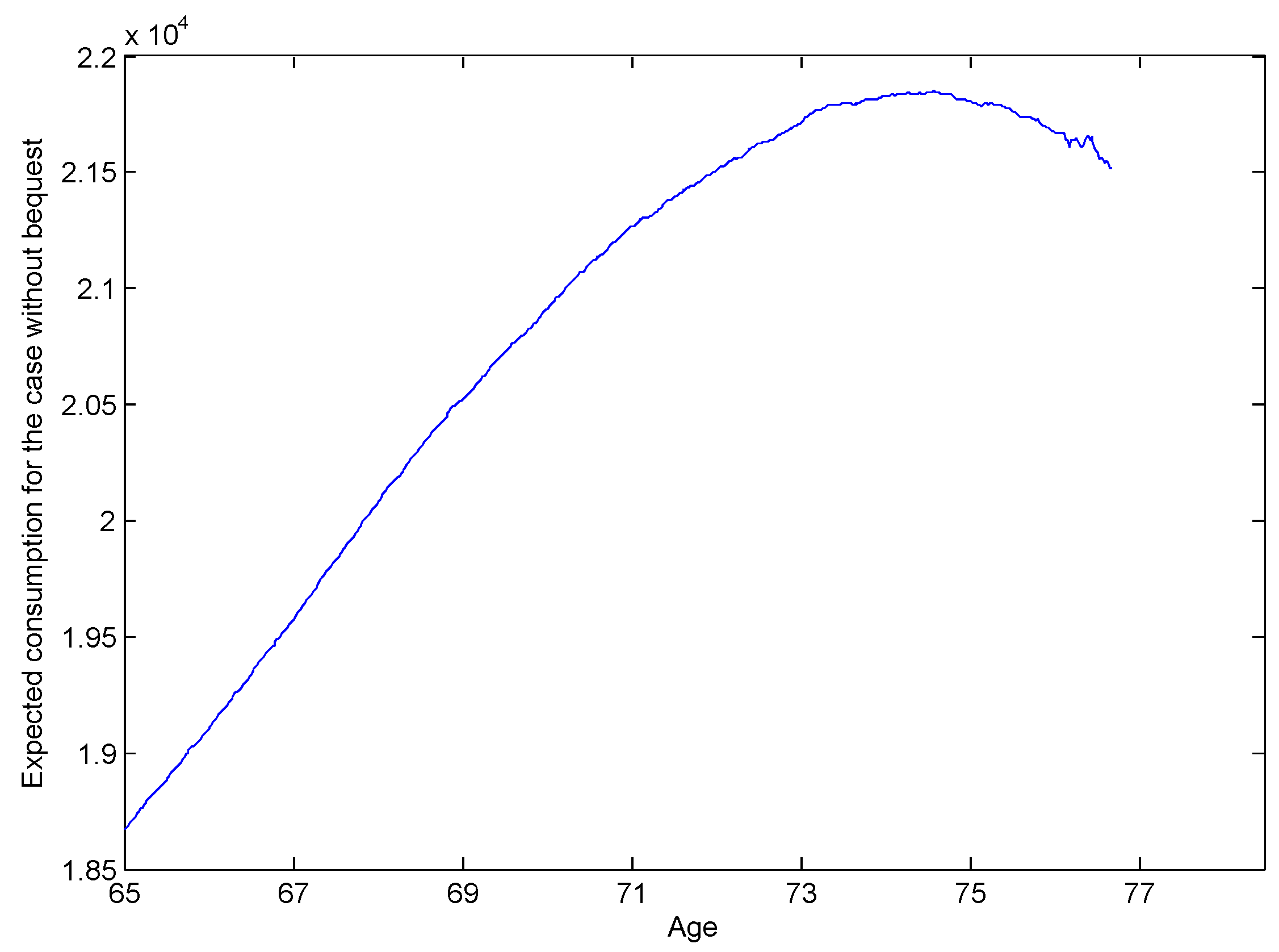
We present the expected consumption path for case 1 in Figure 1. From the plot, we see the expected consumption path is hump-shaped—similar to consumption observed in empirical studies [44,45]. This phenomenon can be attributed to both market incompleteness (lack of access to insurance markets) and low wealth levels in the later life stages.

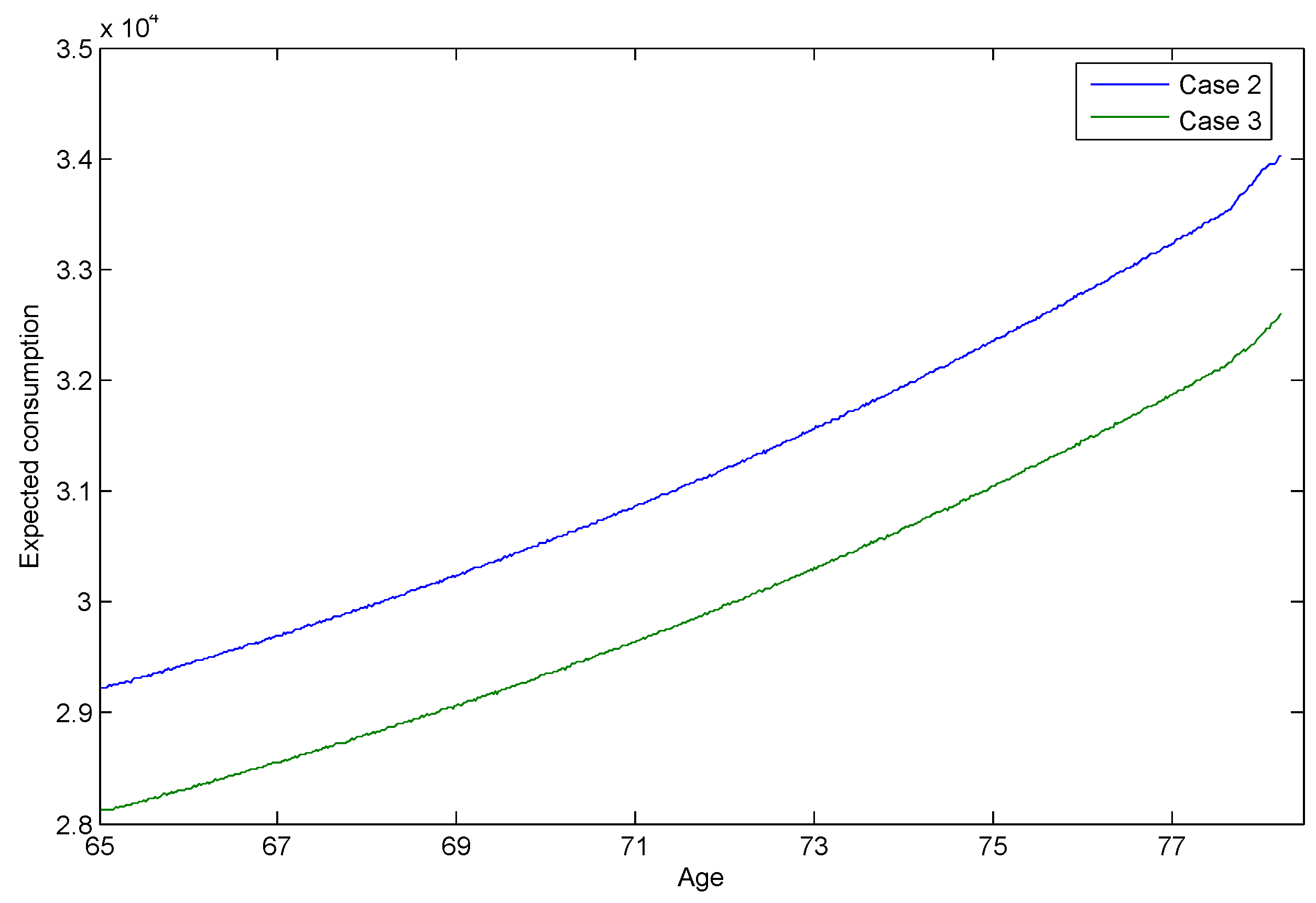
In Figure 2, the expected consumption for cases 2 and 3 rises in line with increasing age. Due to uncertainty arising from the unknown future health state, the market is not entirely complete and thus expected consumption is slightly convex. Compared to Figure 1, Figure 2 reflects the ability of retirees in cases 2 and 3 who have bequest motives to spend more on consumption as they have access to an active insurance market to carry out annuitisation or to purchase insurance. Figure 2 also shows that retirees in case 3 have less consumption than those in case 2, due to the cost of replication of the American put option to ensure they can clear the wealth hurdle required for entry.

Our calculations indicate health changes impact optimal consumption decisions. As one would expect, agents in the poorer health state consume more than those in the healthy state.

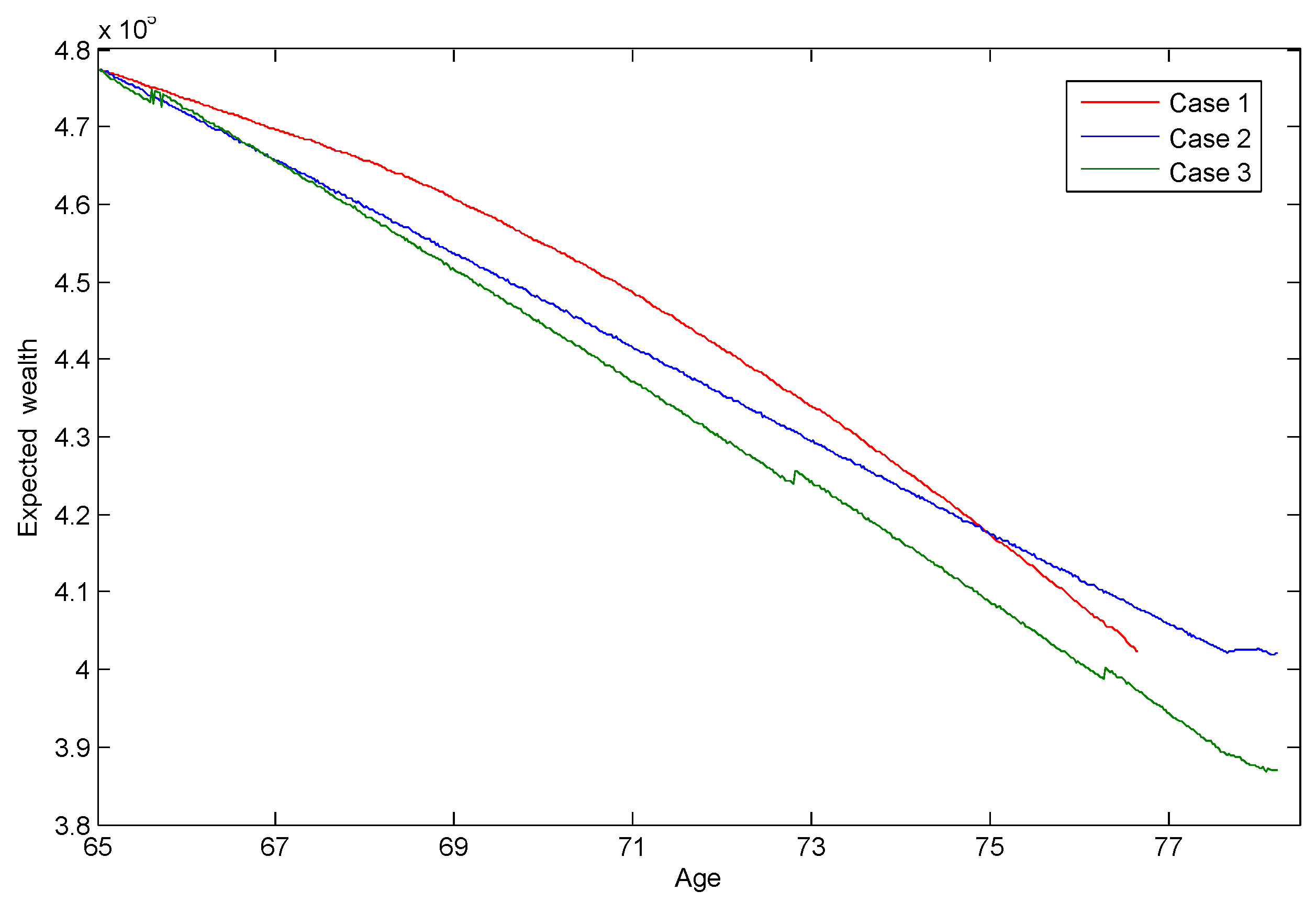
We display the expected wealth path for cases 1, 2 and 3 in Figure 3. For most of time, retirees in case 1 are in possession of more expected wealth than those in case 2 and case 3. As there is no active insurance market in case 1, self-insurance due to precautionary motives is found to be another driver for holding wealth [46]. Hence, Figure 3, suggests retirees tend to draw on their wealth more cautiously when there is no active insurance market. Moreover, the wealth floor requirement in case 3 demands more outgoes and results in less wealth.

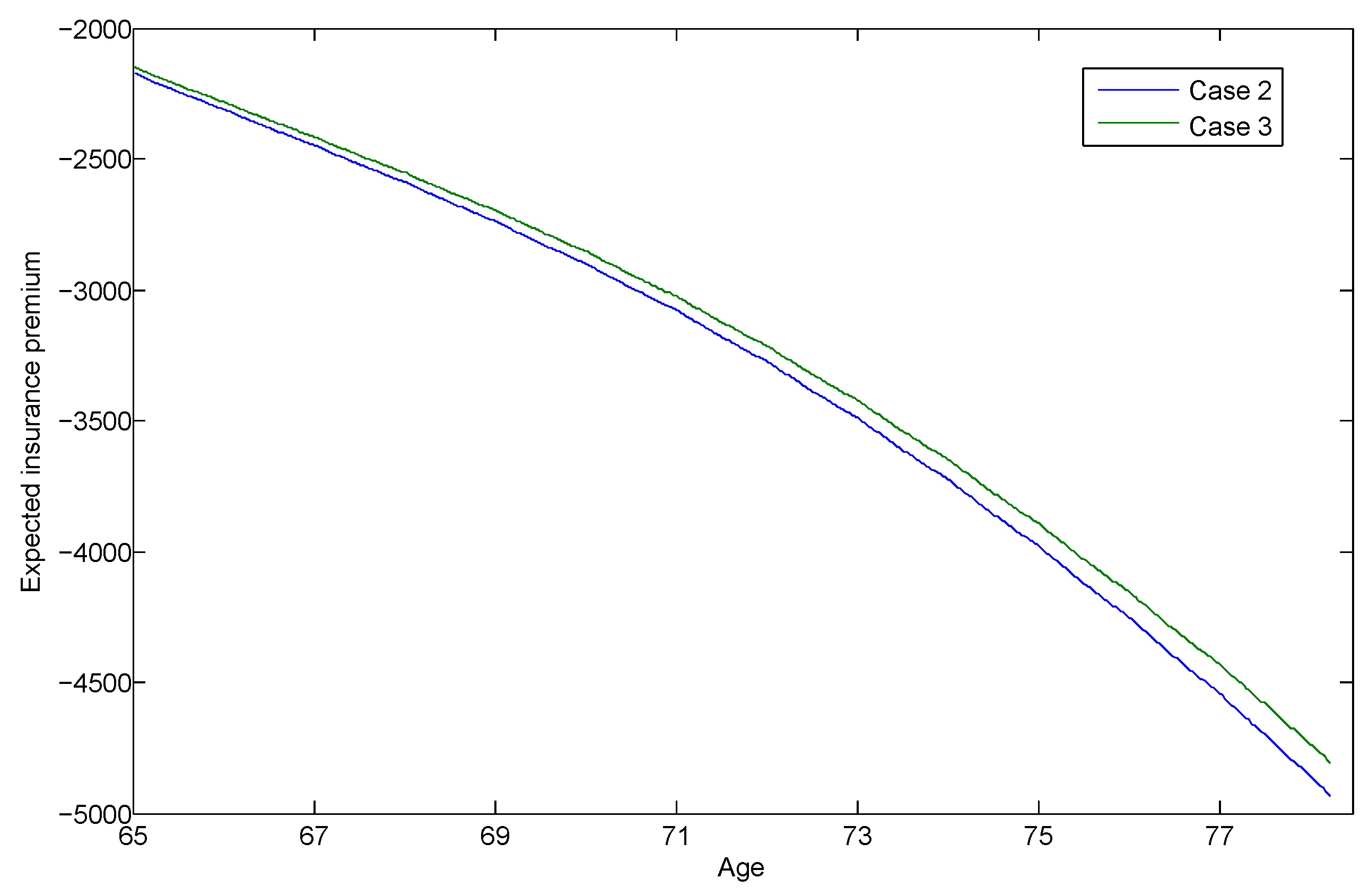
The expected insurance premiums for life insurance or receipt of variable annuity income for cases 2 and 3 are displayed in Figure 4. A positive or negative premium value is linked to the demand for life insurance or a variable annuity, respectively. In Figure 4, retirees in cases 2 and 3 are shown to purchase a variable annuity in order to maximise utility. Compared to those in case 2, retirees in case 3 have a lower annuitisation amount, reflecting the resources they have to put toward replicating the American put option to secure their retirement village entry.

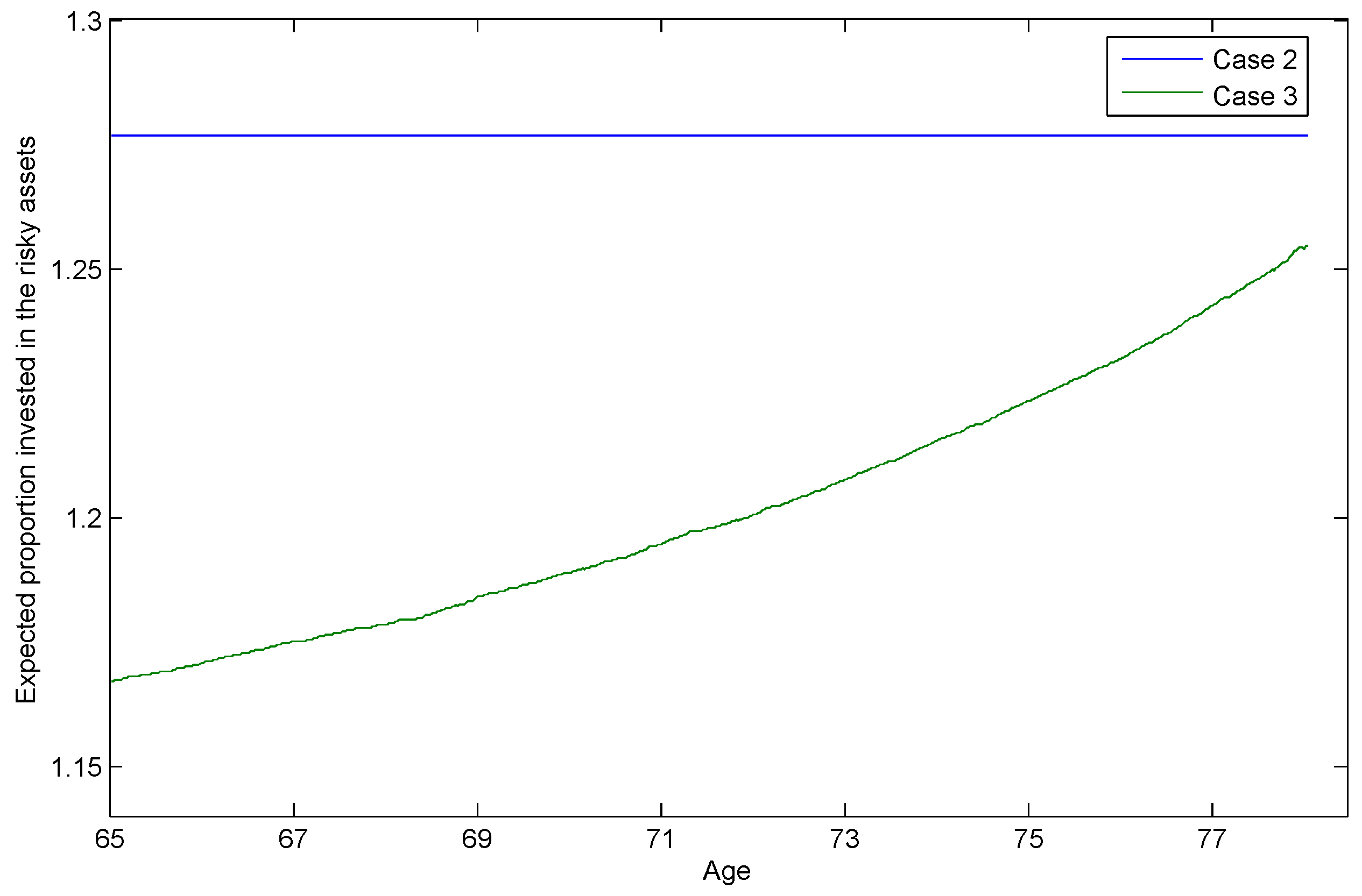
We calculate the proportions of total wealth in risky assets for cases 2 and 3, and display the expected paths of the proportion of surplus wealth, $\tilde{W}$, invested in the risky assets in Figure 5. Retirees in case 2 appear to invest a constant proportion of surplus wealth in risky assets, very much in line with the Merton ratio [15,16]. Indeed, the high values seen are characteristic of the Merton ratio for the parameters chosen and also reflect the lack of short-selling/borrowing restrictions in the modelling. The situation is very different for retirees in case 3 who are target savers and who are assumed to replicate an American put option to meet their target. These retirees, who want to hedge risk, are encouraged to have an increasing risk exposure while they are ageing4. In Figure 5, the proportion of surplus wealth for case 3 rises along with age, producing a convex shape. This trend is similar to that reported in the study by Ding et al. [17], in which retirees are assumed to replicate a European put option for their wealth requirement.

Health changes are seen not to impact investment decisions for our health myopic agents as we chose a level of risk aversion, $\gamma$, that was constant between health states. It should be clear from our myopic health modelling above that if this value differed between states then this would lead to investment behaviour that differed between states. That is, if investors were more risk averse in the sick state, then they would also invest less in the risky assets (compare Merton ratios).

We also test the impacts of some variables on optimal stopping times. As shown in

Table 2. Expected stopping times by level of risk aversion for case 1 and case 2 agents aged 65, in the healthy state, and with total wealth of 10Y—and other parameters as given in Table 1. Increasing levels of risk aversion lead to falling stopping times. Also, the bequest motives of case 2 agents produce results much more sensitive to the level of risk aversion. Indeed, at $\gamma =-0.5$ case 2 agents abandon their conservative behaviour and embrace the risky investment environment.

	Expected Stopping Time (Years)
Gamma	Case 1	Case 2
$-0.5$	11.65	13.22
$-0.6$	11.04	10.53
$-0.7$	10.56	8.28
$-0.8$	10.04	6.23
$-0.9$	9.54	4.50
$-1$	9.13	2.99

, we try different risk-aversion parameter values for case 1, that is, no bequest motive and an incomplete insurance market, and case 2, that is, with bequest motives and a complete insurance market, respectively. With an increasing risk-aversion level for both cases, retirees are shown to be more afraid of potential risks in the markets and prefer an earlier stopping time. The stopping times for case 2 are more sensitive to change in the risk-aversion parameter value. This phenomenon can be explained by the extra risk aversion generated by the bequest motive utility function.

Table 3. Expected stopping times by level of equity premium for case 1 and case 2 agents aged 65, in the healthy state, and with total wealth of 10Y—and other parameters as given in Table 1. Increasing the equity premium results in longer stopping times, as agents exploit the more profitable investment environment. The situation illustrated is for agents with risk aversion of $\gamma =-0.5$, where case 2 agents are less conservative than case 1 agents. With more risk averse agents, this boldness of agents with bequest motives over those without is reversed.

	Expected Stopping Time (Years)
$\mathit{\alpha }-\mathit{r}$	Case 1	Case 2
0.02	5.49	6.38
0.03	7.76	9.02
0.04	10.07	11.60
0.05	12.27	13.87
0.06	14.31	16.06

shows the results of our tests on the impact of excess returns, $\alpha -r$, on the stopping time for case 1, that is, no bequest motive and an incomplete insurance market, and case 2, that is, with bequest motives and a complete insurance market, respectively. As we expected, higher excess returns are more attractive to retirees and defer the stopping time for both cases. This trend can be also found in [21].

The impact of volatility, $\sigma$, on the stopping time for case 1 and case 2 is demonstrated in

Table 4. Expected stopping times by level of market volatility for case 1 and case 2 agents aged 65, in the healthy state, and with total wealth of 10Y—and other parameters as given in Table 1. Increasing market volatility results in shorter stopping times, as agents shy away from the riskier environment. The situation illustrated is for agents with risk aversion of $\gamma =-0.5$, where case 2 agents are less conservative than case 1 agents. With more risk averse agents, this boldness of agents with bequest motives over those without is reversed.

	Expected Stopping Time (Years)
$\mathit{\sigma }$	Case 1	Case 2
0.12	14.62	16.45
0.13	13.67	15.46
0.14	13.44	14.51
0.15	12.10	13.70
0.16	11.42	12.99

. For both two cases, retirees are seen to enter the retirement village earlier when the market is more volatile.

As shown in

Table 5. Expected stopping times by frailty factor u for case 1 and case 2 agents aged 65, in the healthy state, and with total wealth of 10Y—and other parameters as given in Table 1. Increasing frailty results in shorter stopping times, as less healthy agents choose the safer retirement village world sooner. The situation illustrated is for agents with risk aversion of $\gamma =-0.5$, where case 2 agents are less conservative than case 1 agents. With more risk averse agents, this boldness of agents with bequest motives over those without is reversed.

	Expected Stopping Time (Years)
$\mathit{u}$	Case 1	Case 2
1.1	13.40	14.15
1.2	11.65	13.22
1.3	10.15	12.38
1.4	8.85	11.58

, we also study the impact of the frailty factor on the stopping time. In both case 1 and case 2, when retirees are more frail in the sick state, and consequently have more mortality risk, they intend to stop earlier. These findings are in line with [49], who uses a very different (actuarial) approach, to discover that retirees entering retirement villages when they are younger and healthier are financially better off.

5. Conclusions

This paper provides an innovative contribution in its investigation of several cases of retirees entering retirement villages by using Richard’s model with a HARA utility function and dynamic health states. In our research, in which the time of entering the retirement village is the stopping time, we study the optimal strategy with the optimal stopping time for retirees.

We make several different assumptions for bequest motives and the insurance market to mimic the options faced by retirees when entering retirement villages in the real world. In studying these problems we obtain numerical results of consumption, wealth, insurance premiums and stopping times. In our generalised model retirees are assumed to have require a minimum level of consumption as well as facing a future of dynamic health changes and medical costs.

Retirees are found to have divergent consumption and stopping time trends, when the assumptions of bequest motives and the insurance market change. If retirees are assumed to have a bequest motive and access to insurance and annuity products, they are found to annuitise their excess wealth and to have a higher level of consumption. Otherwise, retirees are shown to have less consumption and to hold more wealth for precautionary purposes. Our numerical results indicate the importance of complete insurance markets for self-reliance in retirement—for increasing the consumption level prior to full annuatisation. This finding implies that the existence of a life insurance market for retirees is essential and critical for retirees’ financial strategy. Our finding supports the argument of Blake [35] and others for deepening insurance and annuity markets. A new research direction is then suggested in the insurance market in relation to the ageing problem. Stopping times are also impacted by the risk-aversion parameter, excess returns and the frailty factor.

In this paper, we also study the investment proportion in risky assets. In the case where there is a wealth requirement (wealth floor), retirees are assumed to replicate an American put option. In our numerical results, retirees are shown to be more conservative and have an increasing proportion of wealth invested in risky assets in line with their increasing age. This result once again verifies the findings in the existing literature.

References

1. World Health Organization (WHO). “World Report on Ageing and Health.” 2015. Available online: http://apps.who.int/iris/bitstream/10665/186463/1/9789240694811_eng.pdf?ua=1 (accessed on 4 July 2016).
2. Australian Institute of Health and Welfare. “Australia’s Welfare 2013: In Brief.” 2013. Available online: http://www.aihw.gov.au/WorkArea/DownloadAsset.aspx?id=60129544075 (accessed on 5 July 2016). [Google Scholar]
3. Australian Government. “Australia’s Demographic Challenges.” 2004. Available online: http://demographics.treasury.gov.au/content/discussion.asp (accessed on 4 July 2016). [Google Scholar]
4. Australian Institute of Health and Welfare. “Patterns in Use of Aged Care: 2002–03 to 2010–11.” 2014. Available online: http://www.aihw.gov.au/WorkArea/DownloadAsset.aspx?id=60129548006 (accessed on 5 July 2016). [Google Scholar]
5. Australian Institute of Health and Welfare. “The Residential Aged Care and Aged Care Packages in the Community 2012–13 Web Report.” 2014. Available online: http://www.aihw.gov.au/aged-care/residential-and-community-2012-13/ (accessed on 5 July 2016). [Google Scholar]
6. A.P. Glass, and J. Skinner. “Retirement communities: We know what they are … or do we? ” J. Hous. Elderly 27 (2013): 61–88. [Google Scholar] [CrossRef]
7. M. Bernard, B. Bartlam, J. Sim, and S. Biggs. “Housing and care for older people: Life in an English purpose-built retirement village.” Ageing Soc. 27 (2007): 555–578. [Google Scholar] [CrossRef]
8. Property Council of Australia. “Retirement Villages and Residential Aged Care Facilities Compared.” 2013. Available online: http://www.retirementliving.org.au/industry/services/facts/ (accessed on 5 July 2016).
9. J. McDonald. “Community participation in an Australian retirement village.” Aust. J. Ageing 15 (1996): 167–171. [Google Scholar] [CrossRef]
10. L.R. Buys. “Life in a retirement village: Implications for contact with community and village friends.” Gerontology 47 (2000): 55–59. [Google Scholar] [CrossRef]
11. P. Kingston, M. Bernard, S. Biggs, and H. Nettleton. “Assessing the health impact of age-specific housing.” Health Soc. Care Community 9 (2001): 228–234. [Google Scholar] [CrossRef] [PubMed]
12. S.R. Lord, S. Castell, J. Corcoran, J. Dayhew, B. Matters, A. Shan, and P. Williams. “The effect of group exercise on physical functioning and falls in frail older people living in retirement villages: A randomized, controlled trial.” J. Am. Geriatr. Soc. 51 (2003): 1685–1692. [Google Scholar] [CrossRef] [PubMed]
13. Property Council of Australia. “Retirement Village Resident Profile.” 2013. Available online: http://www.retirementliving.org.au/industry/services/facts/ (accessed on 5 July 2016).
14. Australian Bureau of Statistics. “Gender Indicators, Australia, Jan 2013. ” Available online: http://www.abs.gov.au/ausstats/[email protected]/Lookup/4125.0main+features3110Jan%202013 (accessed on 5 July 2016).
15. R.C. Merton. “Lifetime portfolio selection under uncertainty: The continuous-time case.” Rev. Econ. Stat. 51 (1969): 247–257. [Google Scholar] [CrossRef]
16. R.C. Merton. “Optimum consumption and portfolio rules in a continuous-time model.” J. Econ. Theory 3 (1971): 373–413. [Google Scholar] [CrossRef]
17. J. Ding, G. Kingston, and S. Purcal. “Dynamic asset allocation when bequests are luxury goods.” J. Econ. Dyn. Control 38 (2014): 65–71. [Google Scholar] [CrossRef]
18. M.E. Yaari. “Uncertain lifetime, life insurance, and the theory of the consumer.” Rev. Econ. Stud. 32 (1965): 137–150. [Google Scholar] [CrossRef]
19. S.F. Richard. “Optimal consumption, portfolio and life insurance rules for an uncertain lived individual in a continuous time model.” J. Financ. Econ. 2 (1975): 187–203. [Google Scholar] [CrossRef]
20. M.A. Milevsky, and V.R. Young. “Annuitization and asset allocation.” J. Econ. Dyn. Control 31 (2007): 3138–3177. [Google Scholar] [CrossRef]
21. G. Kingston, and S. Thorp. “Annuitization and asset allocation with HARA utility.” J. Pension Econ. Financ. 4 (2005): 225–248. [Google Scholar] [CrossRef]
22. P.H. Dybvig, and H. Liu. “Lifetime consumption and investment: retirement and constrained borrowing.” J. Econ. Theory 145 (2010): 885–907. [Google Scholar] [CrossRef]
23. E. Barucci, and D. Marazzina. “Optimal investment, stochastic labor income and retirement.” Appl. Math. Comput. 218 (2012): 5588–5604. [Google Scholar] [CrossRef]
24. H.S. Rosen, and S. Wu. “Portfolio choice and health status.” J. Financ. Econ. 72 (2004): 457–484. [Google Scholar] [CrossRef]
25. B.D. Bernheim, A. Shleifer, and L.H. Summers. “The strategic bequest motive.” J. Political Econ. 93 (1985): 1045–1076. [Google Scholar] [CrossRef]
26. R.D. Edwards. “Health risk and portfolio choice.” J. Bus. Econ. Stat. 26 (2008): 472–485. [Google Scholar] [CrossRef]
27. M. Yogo. “Portfolio choice in retirement: Health risk and the demand for annuities, housing, and risky assets.” J. Monet. Econ. 80 (2009): 17–34. [Google Scholar] [CrossRef] [PubMed]
28. M. De Nardi, E. French, and J.B. Jones. “Why do the elderly save? The role of medical expenses.” J. Political Econ. 118 (2010): 39–75. [Google Scholar] [CrossRef]
29. G. Kingston, and L. Fisher. “Down the retirement risk zone with gun and camera.” Econ. Pap. 33 (2014): 153–162. [Google Scholar] [CrossRef]
30. W.D. Pfau, and M.E. Kitces. “Reducing Retirement Risk With a Rising Equity Glide-Path (12 September 2013).” Available online: http://ssrn.com/abstract=2324930 (accessed on 5 July 2016).
31. S. Haberman, and E. Pitacco. Actuarial Models for Disability Insurance. New York, NY, USA: Chapman & Hall/CRC, 1999. [Google Scholar]
32. S.M. Ross. Introduction to Probability Models. New York, NY, USA: Academic Press, 2007. [Google Scholar]
33. X. Guo. “An explicit solution to an optimal stopping problem with regime switching.” J. Appl. Prob. 38 (2001): 464–481. [Google Scholar] [CrossRef]
34. F. Iskhakov, S. Thorp, and H. Bateman. “Optimal annuity purchases for Australian retirees.” Econ. Rec. 91 (2015): 139–154. [Google Scholar] [CrossRef]
35. D. Blake. “Annuity markets: Problems and solutions.” Geneva Pap. Risk Ins. Issues Pract. 24 (1999): 358–375. [Google Scholar] [CrossRef]
36. J. Zhu. “Dividend Optimization For A Regime-Switching Diffusion Model With Restricted Dividend Rates.” ASTIN Bull. 44 (2014): 459–494. [Google Scholar] [CrossRef]
37. B. Øksendal. Stochastic Differential Equations, 5th ed. Springer Series; New York, NY, USA: Springer, 2003. [Google Scholar]
38. S. Purcal, and J. Piggott. “Explaining low annuity demand: An optimal portfolio application to Japan.” J. Risk Insur. 75 (2008): 493–516. [Google Scholar] [CrossRef]
39. J.Z. Huang, M.G. Subrahmanyam, and G.G. Yu. “Pricing and hedging American options: A recursive investigation method.” Rev. Financ. Stud. 9 (1996): 277–300. [Google Scholar] [CrossRef]
40. Australian Government Actuary. “Australian Life Tables 2010–12: Males. ” Available online: http://www.aga.gov.au/publications/life_table_2010-12/default.asp (accessed on 5 July 2016).
41. S. Su, and M. Sherris. “Heterogeneity of Australian population mortality and implications for a viable life annuity market.” Insur. Math. Econ. 51 (2012): 322–332. [Google Scholar] [CrossRef]
42. Australian Bureau of Statistics. “Household Income and Income Distribution, Australia, 2011–12. ” Available online: http://www.abs.gov.au/AUSSTATS/[email protected]/DetailsPage/6523.02011-12?OpenDocument (accessed on 5 July 2016).
43. Australian Bureau of Statistics. “Household Expenditure Survey, Australia: Summary of Results, 2009–10. ” Available online: http://www.abs.gov.au/AUSSTATS/[email protected]/DetailsPage/6530.02009-10?OpenDocument (accessed on 5 July 2016).
44. P.O. Gourinchas, and J.A. Parker. “Consumption over the life cycle.” Econometrica 70 (2002): 47–89. [Google Scholar] [CrossRef]
45. J. Fernández-Villaverde, and D. Krueger. “Consumption over the life cycle: Facts from consumer expenditure survey data.” Rev. Econ. Stat. 89 (2007): 552–565. [Google Scholar] [CrossRef]
46. J. Ameriks, A. Caplin, S. Laufer, and S. Van Nieuwerburgh. “The joy of giving or assisted living? Using strategic surveys to separate public care aversion from bequest motives.” J. Financ. 66 (2011): 519–561. [Google Scholar] [CrossRef]
47. H. Hulley, R. Mckibbin, A. Pedersen, and S. Thorp. “Means-tested public pensions, portfolio choice and decumulation in retirement.” Econ. Rec. 89 (2013): 31–51. [Google Scholar] [CrossRef]
48. S. Thorp, G. Kingston, and H. Bateman. “Financial engineering for Australian annuitants.” In Retirement Provision in Scary Markets. Edited by H. Bateman. Cheltenham, UK: Northampton, MA, USA: Edward Elgar, 2007, pp. 123–144. [Google Scholar]
49. T. Kyng, and B. Stolz. An Actuarial Analysis of Australian Retirement Village Contracts: Consumer Perspective. Unpublished Paper; Sydney, Australia: Macquarie University, 2016. [Google Scholar]
50. F. Black, and M. Scholes. “The pricing of options and corporate liabilities.” J. Political Econ. 81 (1973): 637–654. [Google Scholar] [CrossRef]
51. L. Wu, and Y.K. Kwok. “A front-fixing finite difference method for the valuation of American options.” J. Financ. Eng. 6 (1997): 83–97. [Google Scholar]
• 1.See, for example, Ross [32].
• 2.Retirees need to pay a large amount in upfront fees to live in such a community and have the right to re-sell the occupation rights of the property.
• 3.Note that P ( t ) > 0 reflects the retiree (continuously) purchasing life insurance, while P ( t ) < 0 indicates the retiree has entered into something akin to a (instantaneous) variable annuity contract with an insurer [38].
• 4.Retirees are also found to use increasing risk exposure to hedge against risk in other studies, such as Hulley et al. [47] and Thorp et al. [48].
Figure 1. Expected consumption path for case 1 retirees, starting in the healthy state at age 65 with total wealth of 10Y, and truncated at the optimal case 1 stopping times. This captures the expected consumption outcomes of agents with no bequest motive. Note that these agents have no access to insurance markets, and are assumed to purchase a term certain annuity to protect their basic consumption needs—which is much more expensive than a life annuity, particularly at older ages.
Risks 05 00020 g001
Figure 2. Expected consumption, truncated at optimal stopping times, for case 2 and case 3 agents commencing at age 65 in the healthy state with total wealth of 10Y. The figure captures the expected consumption paths for agents with bequest motives. These agents, in contrast to case 1, have access to perfect insurance markets.
Risks 05 00020 g002
Figure 3. Expected wealth, truncated at optimal stopping times, for case 1, 2 and 3 agents commencing at age 65 in the healthy state with total wealth of 10Y. Recall case 1 agents have no access to insurance markets, while case 3 agents replicate an American put option to ensure their savings target is met.
Risks 05 00020 g003
Figure 4. Expected insurance premiums paid by case 2 and case 3 agents, truncated at optimal stopping times, for those commencing at age 65 in the healthy state with a total wealth of 10Y. Negative insurance premiums mean the agents are receiving funds from the insurers, that is, they are in receipt of an annuity.
Risks 05 00020 g004
Figure 5. Expected proportion of surplus wealth, W ˜ , invested in the risky assets, or π * W / W ˜ , by agents starting at age 65 in the healthy state with a total wealth of 10Y. The expected paths are truncated at the optimal stopping times for case 2 and case 3, respectively. The differing behaviour of the case 3 target savers is clear.
Risks 05 00020 g005